$k$-$L(2,1)$-Labelling for Planar Graphs is NP-Complete for $k\geq 4$

HAL Id: inria-00360505

https://hal.inria.fr/inria-00360505

Submitted on 11 Feb 2009

HAL is a multi-disciplinary open access

archive for the deposit and dissemination of

sci-entific research documents, whether they are

pub-lished or not. The documents may come from

teaching and research institutions in France or

abroad, or from public or private research centers.

L’archive ouverte pluridisciplinaire HAL, est

destinée au dépôt et à la diffusion de documents

scientifiques de niveau recherche, publiés ou non,

émanant des établissements d’enseignement et de

recherche français ou étrangers, des laboratoires

publics ou privés.

k-L(2, 1)-Labelling for Planar Graphs is NP-Complete for

k

≥ 4

Nicole Eggemann, Frédéric Havet, Steven Noble

To cite this version:

Nicole Eggemann, Frédéric Havet, Steven Noble.

k-L(2, 1)-Labelling for Planar Graphs is

a p p o r t

d e r e c h e r c h e

k-L(2, 1)-Labelling for Planar Graphs is

NP-Complete for k

≥ 4.

Nicole Eggemann — Frédéric Havet — Steven Noble

N° 6840

Centre de recherche INRIA Sophia Antipolis – Méditerranée 2004, route des Lucioles, BP 93, 06902 Sophia Antipolis Cedex

Nicole Eggemann

_{, Fr´ed´eric Havet}

_{, Steven Noble}

Th`eme COM — Syst`emes communicants ´

Equipe-Projet Mascotte

Rapport de recherche n°6840 — F´evrier 2009 — 18 pages

Abstract: A mapping from the vertex set of a graph G = (V, E) into an interval of integers {0, . . . , k} is an L(2, 1)-labelling of G of span k if any two adjacent vertices are mapped onto integers that are at least 2 apart, and every two vertices with a common neighbour are mapped onto distinct integers. It is known that for any fixed k ≥ 4, deciding the existence of such a labelling is an NP-complete problem while it is polynomial for k ≤ 3. For even k ≥ 8, it remains NP-complete when restricted to planar graphs. In this paper, we show that it remains NP-complete for any k ≥ 4 by reduction from Planar Cubic Two-Colourable Perfect Matching. Schaefer stated without proof that Planar Cubic Two-Two-Colourable Perfect Matching is NP-complete. In this paper we give a proof of this.

Key-words: L(2, 1)-labelling, distance contrained colouring, planar graph, complexity, channel assign-ment

∗_{Brunel University, Kingston Lane, Uxbridge, UB8 3PH, UK. Supported by the EC Marie Curie programme NET-ACE}

(MEST-CT-2004-6724).Nicole.Eggemann@brunel.ac.uk

† _{projet Mascotte, I3S(CNRS and University of Nice-Sophia Antipolis) and INRIA, 2004 Route des Lucioles,}

BP 93, 06902 Sophia-Antipolis Cedex, France. Partially supported by the european project FET - Aeolus.

Frederic.Havet@sophia.inria.fr.

‡_{Brunel University, Kingston Lane, Uxbridge, UB8 3PH, UK. Partially supported by the Heilbronn Institute for}

k-L

(2, 1)-Labelling pour les graphes planaires est NP-Complete

pour k

≥ 4.

R´esum´e : Une application de l’ensemble des sommets d’un graphe G = (V, E) dans un intervalle des entiers naturels {0, . . . , k} est un L(2, 1)-labelling de G d’´ecart k si deux sommets adjacents recoivent des entiers `a distance au moins 2 et deux sommets ayant un voisin en commun recoivent des entiers distincts. On sait que pour k ≥ 4, d´ecider l’existence d’un L(2, 1)-labelling est un probl`eme NP-complet pour k ≥ 4 alors que c’est polynomial pour k ≤ 3. Pour k ≥ 8 et pair, cela reste NP-complet restreint `

a la classe des graphes planaires. Dans ce rapport, nous montrons que cela reste NP-complet pour tout k≥ 4 par r´eduction de Planar Cubic Two-Colourable Perfect Matching. Schaefer a affirm´e sans preuve que ce probl`eme est NP-complet. Nous en donnons une preuve ici.

Mots-cl´es : L(2, 1)-labelling, coloration avec contrainte de distance, graphe planaire, complexit´e, allocation de fr´equences

The Frequency Assignment Problem requires the assignment of frequencies to radio transmitters in a broadcasting network with the aim of avoiding undesired interference and minimising bandwidth. One of the longstanding graph theoretical models of this problem is the notion of distance constrained labelling of graphs. An L(2, 1)-labelling of a graph G is a mapping from the vertex set of G into the nonnegative integers such that the labels assigned to adjacent vertices differ by at least 2, and labels assigned to vertices at distance 2 are different. The span of such a labelling is the maximum label used. In this model, the vertices of G represent the transmitters and the edges of G express which pairs of transmitters are too close to each other so that an undesired interference may occur, even if the frequencies assigned to them differ by 1. This model was introduced by Roberts [11] and since then the concept has been intensively studied (see the survey of Yeh [13]).

In their seminal paper, Griggs and Yeh [7] proved that determining the minimum span of a graph G, denoted λ2,1(G), is an NP-hard problem. Fiala et al. [5] proved that deciding λ2,1(G) ≤ k is NP-complete

for every fixed k ≥ 4 and later Havet and Thomass´e [8] proved that for any k ≥ 4, it remains NP-complete when restricted to bipartite graphs (and even a restricted family of bipartite graphs, i.e incidence graphs or first division of graphs). When the span k is part of the input, the problem is nontrivial for trees but a polynomial time algorithm based on bipartite matching was presented in [3]. The problem is still solvable in polynomial time if the input graph is outerplanar [9, 10].

Moreover, somewhat surprisingly, the problem becomes NP-complete for series-parallel graphs [4], and thus the L(2, 1)-labelling problem belongs to a handful of problems known to separate graphs of tree-width 1 and 2 by P/NP-completeness dichotomy.

In this paper we consider the following problem. Problem 0.1(Planar k-L(2, 1)-Labelling).

Let k ≥ 4 be fixed.

Instance: A planar graph G.

Question: Is there an L(2, 1)-labelling with span k?

Bodlaender et al. [1] showed that this problem is NP-complete if we require k ≥ 8 and k even. In the survey paper [2], it is suggested that the problem is NP-complete for all k ≥ 8 due to [6]. However this does not seem to be the case. In [6] there is a proof showing that the corresponding problem where kis specified as part of the input is NP-complete. This proof shows that the problem is NP-complete for certain fixed values of k. However it is far from clear for which values of k this is true.

In this paper we first prove that Planar Cubic Two-Colourable Perfect Matching, which we define in the next section, is NP-Complete. This result was first stated by Schaefer [12] but without proof. In the second part of this paper we use this result in order to show that Problem 0.1 is NP-complete.

1

Preliminary results

The starting problem for our reductions is Not-All-Equal 3SAT, which is defined as follows [12]. Definition 1.1 (Not-All-Equal 3SAT).

Instance: A set of clauses each having three literals.

Question: Can the literals be assigned value true or false so that each clause has at least one true and at least one false literal?

In [12], it is shown that this problem is NP-complete.

Our reduction involves an intermediate problem concerning a special form of two-colouring. In this section we define the intermediate problem and show that it is NP-complete. When k = 4 or k = 5, the final stage of our reduction is similar to the reduction in [5]. However we cannot use induction for higher

4 N..Eggemann, F. Havet, and S. Noble a b c d e f g h i j k l o p q r m n

Figure 1: Planar graph H.

values of k in contrast with the situation in [5] and the problem from which the reduction starts in [5] is not known to be NP-complete for planar graphs. So considerably more work is required.

The following problem is also discussed in [12].

Problem 1.2(Two-Colourable Perfect Matching). Instance: A graph G.

Question: Is there a colouring of the vertices of G with colours black and white in which every vertex has exactly one neighbour of the same colour?

In [12] it was shown that Two-Colourable Perfect Matching is NP-complete. We are more interested in the case where the input is restricted to being a planar cubic graph. We call this variant, Planar Cubic Two-Colourable Perfect Matching defined formally as follows [12].

Problem 1.3(Planar Cubic Two-Colourable Perfect Matching). Instance: A planar cubic graph G.

Question: Is there a colouring of the vertices of G with colours black and white in which every vertex has exactly one neighbour of the same colour?

Schaefer [12] states that this problem is NP-complete but does not give the details of the proof. We call a colouring as required in Problem 1.3 a two-coloured perfect matching. This section is devoted to the proof of this result, using a reduction from Not-All-Equal 3SAT [12]. As far as we know, no proof of this has ever been published.

We say that a colouring of the vertices of a graph with colours black and white is an almost two-coloured perfect matching if every vertex of degree at least two is adjacent to exactly one vertex of the same colour. We say an edge is monochromatic if both endpoints have the same colour and dichromatic if its endpoints have different colours.

Let H be the planar graph (see Fig. 1) with

V(H) = {a, b, c, d, e, f, g, h, i, j, k, l, m, n, o, p, q, r} and

E(H) = {ab, bc, bd, ce, cf, dg, dh, ef, gh, ei, f j, gk, hl, im, jk, ln, io, jo, oq, kp, pl, pr}.

H plays a key role in showing that Problem 1.3 is NP-complete. We need the following lemma. Lemma 1.4. Any almost two-coloured perfect matching of H has the following properties.

ˆ Exactly one of the edges ab, mi, ln is monochromatic.

Figure 2: Three almost two-coloured perfect matchings of the subgraph of H induced by the vertices c, e, f, m, i, j, k, o, p.

Figure 3: Almost two-coloured perfect matchings of H.

ˆ Vertices b, i, l receive the same colour.

ˆ Vertices o, p, q, r receive the other colour to b, i, l.

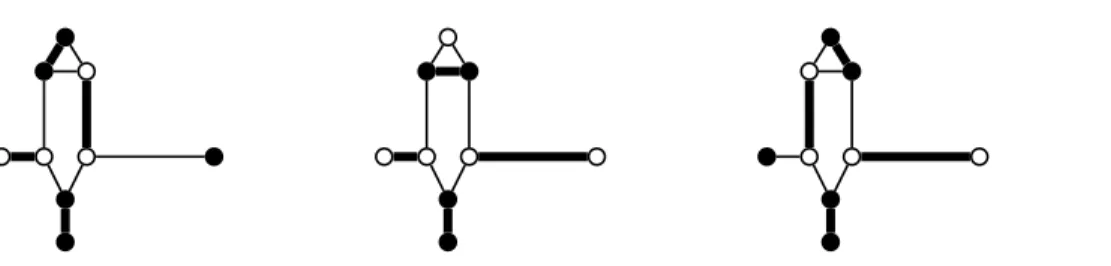
Proof. Consider the triangles on the vertices c, e, f and g, h, d. In order to obtain an almost two-coloured perfect matching exactly one of the edges ce, ef and cf must be monochromatic. The same is true for the triangle on the vertices g, h, d. Now consider the subgraph of H induced by the vertices c, e, f, i, j, m, k, o, q. In Fig. 2 three of the six almost two-coloured perfect matchings of this subgraph are depicted with monochromatic edges shown by heavy lines. The other three two-coloured perfect matchings are obtained by interchanging the colours. It follows that oq and pr must be monochromatic. By symmetry the same applies to the subgraph of H induced by the vertices d, g, h, j, k, l, n, p, r. Considering which pairs of these almost two-coloured perfect matchings are compatible and extend to an almost two-coloured perfect matching of H shows that there are only six possibilities. In Fig. 3 three possible two-coloured almost perfect matchings are depicted. The only other possible two-coloured almost perfect matchings are obtained by interchanging the two colours. Clearly these all have the properties described in the lemma.

We define what we call the clause gadget graph K as follows, see Fig. 4. Take three copies of H, namely H1, H2 and H3. We label the vertices by adding the subscript i ∈ {1, 2, 3} to the corresponding

label of H. Now identify a1, a2, a3into a single vertex a, remove vertices m1, m2, m3, n1, n2, n3 and their

incident edges and replace them with edges l1i2, l2i3, l3i1. Notice that K is planar and every vertex has

degree three, except for q1, q2, q3 and r1, r2, r3.

Lemma 1.5. A two-colouring of S3t=1{ot, qt, pt, rt} ∪ {a} may be extended to an almost two-coloured

perfect matching of K if and only if

ˆ For each t = 1, 2, 3, otqt, ptrt are monochromatic and ot, pt, qt, rt all receive the same colour. ˆ For exactly two values of t = 1, 2, 3, the vertices ot, pt, qt, rt receive the same colour as a.

6 N..Eggemann, F. Havet, and S. Noble a b1 b2 b3 l1 i1 l3 i3 i2 l2

Figure 4: Planar clause gadget K.

Proof. We first show that any almost two-coloured perfect matching of K must have the two properties in the lemma.

The first property is an immediate consequence of Lemma 1.4.

To show that the second property holds, recall that exactly one neighbour of a must receive the same colour as a. Let bt1 for 1 ≤ t1 ≤ 3 be this neighbour. Then from Lemma 1.4 we know that bt1

must have the opposite colour to ot1, pt1, qt1, rt1. Since the other neighbours of a, namely bt2 and bt3

for t2, t3∈ {1, 2, 3}\{t1}, receive the opposite colour to a, ot2, pt2, qt2, rt2, ot3, pt3, qt3, rt3 must receive the

same colour as a.

Now we show that any two-colouring ofS3_t=1{ot, qt, pt, rt, bt} ∪ {a} satisfying the conditions of the

lemma may be extended to an almost two-coloured perfect matching of K. Suppose without loss of generality, a is coloured black and o1, p1, q1, r1are coloured white. Then colour l1, i1black and l2, i2, l3, i3

white. This colouring may be extended to an almost two-coloured perfect matching using the colourings of Fig. 3 and the colourings obtained from those in Fig. 3 by interchanging the colours.

We now move a step towards the main result of this section with the following proposition. Proposition 1.6. Problem 1.2 is NP-complete if the input is restricted to cubic graphs.

Proof. Given an instance of Not-All-Equal 3SAT with clauses C1, ..., Cm, construct a graph as follows.

For every clause C take a copy of the clause gadget graph K and do the following. Suppose without loss of generality C has literals x1, x2, x3. Label the two vertices of degree one of the subgraph Hi of K(C)

and their neighbours in Hi with xi.

Now for each literal x do the following. Suppose that literal x appears in clauses Ci1, ..., Cik. (If

xappears twice or three times in a clause Cr then add Cr twice or three times to this list.) For every

j= 1, ..., k − 1 remove either one of the vertices of degree one labelled x from K(Cij) and from K(Cij+1)

leaving two half-edges. Now identify these two half edges to form an edge joining K(Cij) and K(Cij+1).

Finally do the same thing with the remaining two edges labelled x in Cik and Ci1. We call the graph

obtained G.

Now suppose that there is a solution S of the instance of Not-All-Equal 3SAT given. For all literals xin Not-All-Equal 3SAT, colour all vertices in G that are labelled x with colour white if S(x) is true and black if S(x) is false. We now show that this colouring can be extended to a two-coloured perfect matching of G. First note that all edges joining copies of K are monochromatic since their endpoints

z4 z3 u x n q l m p r v w k o f i e d j h c g b a s t z1 z2 α α α′ α′ α α β′ β β′ β β β α′ _α′ α α β′ β β β′ α′ α′ α α β′ β′ β β

Figure 5: Uncrossing gadget U and its possible almost two-coloured perfect matchings where α, β ∈ {black, white} and α′_{, β}′ _{are the opposite colours to α and β, respectively.}

are labelled with the same literal. In the next step colour the vertex a in each copy of K so that it has the same colour as the vertices ot, pt for exactly two values of t = 1, 2, 3. This is possible because for

t= 1, 2, 3 ot, pt are labelled with literals x1, x2, x3 which cannot have all the same value as they belong

to one clause. By Lemma 1.5 we can extend the colouring of each copy of K to an almost two-coloured perfect matching of K which yields a two-coloured perfect matching of G.

Now suppose there is a two-coloured perfect matching of G. By Lemma 1.5 the edges joining the copies of K must be monochromatic. All vertices in G labelled with the same literal therefore must have the same colour and in each copy of K, for exactly two values of t = 1, 2, 3, the vertices ot, ptreceive the

same colour. It follows that if we assign to each literal x the value true if it is the label of white vertices and false it is the label of black vertices then we obtain a solution to Not-All-Equal 3SAT.

We call the edges joining copies of K identifying edges.

In order to prove that Problem 1.3 is NP-complete we still need to deal with edges that cross. For this reason we define the uncrossing gadget U as follows, see Fig. 5.

V(U ) = {a, b, c, d, e, f, g, h, i, j, k, l, m, n, o, p, q, r, s, t, u, v, w, x, z1, z2, z3, z4}

and

E(U ) = {ab, bc, bg, ce, cd, ef, df, dh, gh, hi, gj, ij, f k, kl, km, ln, mn, mp, io, op, or, pq, rq, ev, lv, wv, js, rt, st, sz1, tz1, z1z2, nu, qx, ux,

uz3, xz3, z3z4}.

Lemma 1.7. There exists an almost two-coloured perfect matching of U if and only if w, v, z1, z2 have

the same colour and a, b, z3, z4 have the same colour.

Proof. Consider the four-cycle on the vertices c, e, f, d in U . In a two-coloured perfect matching exactly two of the vertices c, e, f, d must receive the colour black and the other two must receive the colour white. There are two different ways of colouring them. The first way is that exactly two of the edges in the

8 N..Eggemann, F. Havet, and S. Noble

Figure 6: Sketch of the modification from the Not-All-Equal 3SAT problem to a planar cubic graph .

four-cycle are monochromatic, namely ce and df , or cd and ef . Then none of the edges cb, dh, ev, f k can be monochromatic. The other way is that none of the edges in the four-cycle is monochromatic and all of the edges cb, dh, ev, f k are monochromatic. The analogous thing is true for any four-cycle in U .

We now prove that in any almost two-coloured perfect matching the edges ab, wv, z1z2and z3z4are

monochromatic. Suppose ab is dichromatic. Then precisely one of bc and bg must be monochromatic. Without loss of generality assume bc is monochromatic. Then the four-cycle on c, e, f, d cannot have a monochromatic edge. It follows dh must be monochromatic. But then bg must be monochromatic which is a contradiction. Thus ab and by symmetry wv must be monochromatic. Now suppose z1z2is dichromatic.

It follows that precisely one of sz1 and tz1 is monochromatic. Without loss of generality assume tz1 is

monochromatic. Then js must be monochromatic. It follows that io must be monochromatic and so must rt. This is not possible. Thus z1z2and due to symmetry z3z4must be monochromatic. Hence each

of the four-cycles (c, d, f, e), (g, h, i, j), (k, l, n, m), (o, p, q, r) contains exactly two monochromatic edges. So vertices that are opposite of each other in these four-cycles receive opposite colours. It is now easy to see that the only possible colourings are as shown in Fig. 5 where α, β ∈ {black, white} and α′ _denotes

the opposite colour to α and β′ _{denotes the opposite colour to β. The result then follows.}

Our next result was originally stated without proof in [12]. To the best of our knowledge no proof of this result has ever been published. In [12] a reduction from Not-All-Equal 3SAT is used to show that the version of Problem 1.3 where the input may be any graph is NP-complete. We use a reduction from Not-All-Equal 3SAT in a similar way but with much more complicated gadgets.

Theorem 1.8. Problem 1.3 is NP-complete.

Proof. Given an instance of Not-All-Equal 3SAT, construct the graph G as in the proof of Proposition 1.6. This graph can be drawn in the plane so that the only edges that cross are the identifying edges, each pair of identifying edges crosses at most once and at most two edges cross at any point.

Now we replace the crossings one by one by replacing a pair of crossing edges by the uncrossing gadget, see Fig. 6. Suppose γ and δ are two edges that cross. We delete γ and δ and replace them with

a copy of the uncrossing gadget attaching w and z2to the endpoints of γ, and a and z4 to the endpoints

of δ. We will also call the four pendant edges wv, ab, z1z2, z3z4 in the uncrossing graph identifying

edges. After each replacement we can draw the graph so that only identifying edges cross and such that there is one fewer crossing. We continue until there are no more crossing edges. The final graph can be constructed in polynomial time and is planar and cubic. Each original identifying edge in G now corresponds to one or more identifying edges with each consecutive pair being on opposite sides of a copy of the uncrossing gadget. Lemma 1.7 shows that in a two-coloured perfect matching all of these edges must be monochromatic and all the endpoints of these edges have the same colour.

Now the argument in Proposition 1.6 shows that the final graph has a two-coloured perfect matching if and only if the instance of Not-All-Equal 3SAT is satisfiable.

2

k-L

(2, 1)-labelling for k ≥ 4 fixed

Let G be a planar cubic graph. In order to establish our main result we will reduce Planar Cubic Two-Colourable Perfect Matching to Planar k-L(2, 1)-Labelling for planar graphs for each k ≥ 4. From any planar cubic graph G forming an instance of Planar Cubic Two-Colourable Perfect Matching, we construct a graph K. As we see in the next section, the basic form of K does not depend on k but is formed by constructing an auxiliary graph H and then replacing each edge of H by a gadget which does depend on k. In this section we define these gadgets and analyse certain L(2, 1)-labellings of them. Each gadget has two distinguished vertices, which will always be labelled u and v, corresponding to the endpoints of the edge that is replaced in the auxiliary graph defined in the next section. These two vertices have degree k− 1 in K. Any vertex of degree k − 1 must receive either label 0 or k in a k-L(2, 1)-labelling because these are the only possible labels for which there are k − 1 labels remaining to label the neighbours of that vertex, so we will analyse the k-L(2, 1)-labellings of these gadgets in which u, v receive label 0 or k.

2.1

λ

(G) = 4

In this subsection the gadget G4is simply a path of length three. More precisely the gadget G4is given

by

V(G4) = {u, au, av, v}

and

E(G4) = {uau, auav, avv}.

This gadget is used in [5], from where we get the following lemma.

Lemma 2.1. There is a 4-L(2, 1)-labelling L of G4 with L(u), L(v) ∈ {0, 4} if and only if the following

conditions are satisfied.

(i) If (L(u), L(v)) = (0, 0), then (L(au), L(av)) ∈ {(2, 4), (4, 2)}.

(ii) If (L(u), L(v)) = (4, 4), then (L(au), L(av)) ∈ {(0, 2), (2, 0)}.

(iii) If (L(u), L(v)) = (4, 0), then (L(au), L(av)) = (1, 3).

10 N..Eggemann, F. Havet, and S. Noble u au av v bv bu c d e3 e1 e2 f g1 g2

Figure 7: The edge gadget G5.

2.2

λ

(G) = 5

Let G5be the graph as depicted in Fig. 7.

Lemma 2.2. There is a 5-L(2, 1)-labelling L of G5 with L(u), L(v) ∈ {0, 5} if and only if the following

conditions are satisfied.

(i) If (L(u), L(v)) = (0, 0) then (L(au), L(av)) ∈ {(2, 5), (5, 2), (3, 5), (5, 3)}.

(ii) If (L(u), L(v)) = (5, 5) then (L(au), L(av)) ∈ {(3, 0), (0, 3), (2, 0), (0, 2)}.

(iii) If (L(u), L(v)) = (0, 5) then (L(au), L(av)) = (4, 1).

(iv) If (L(u), L(v)) = (5, 0) then (L(au), L(av)) = (1, 4).

Proof. (i) By the definition of L(2, 1)-labelling, L(au) and L(av) are both in {2, 3, 4, 5}. As |L(au) −

L(av)| ≥ 2 then (L(au), L(av)) ∈ {(2, 4), (4, 2), (2, 5), (5, 2), (3, 5)(5, 3)}.

Suppose for a contradiction that (L(au), L(av)) ∈ {(2, 4), (4, 2)}. By symmetry, we may assume

that (L(au), L(av)) = (2, 4). Then L(bu) = 5 and L(bv) = 1. The vertices d and f have degree four

and thus must receive labels from {0, 5}. Because dist (bu, d) = 2 we must have L(d) = 0 and because

dist (d, f ) = 2 we must have L(f ) = 5. This implies that {L(e1), L(e2)} = {2, 3}. But then vertex c

cannot be labelled, giving a contradiction. An L(2, 1)-labelling is obtained if (L(au), L(av)) = (5, 2) and

L(bu) = 3, L(bv) = 4, L(c) = 0, L(d) = 5, L(e3) = 1, L(e2) = 2, L(e1) = 3, L(f ) = 0 L(g1) = 5

and L(g2) = 4 or if (L(au), L(av)) = (5, 3) and L(bu) = 2, L(bv) = 1, L(c) = 4, L(d) = 0, L(e3) = 5,

L(e2) = 2, L(e1) = 3, L(f ) = 5 L(g1) = 0 and L(g2) = 1. The other cases follow by symmetry.

(ii) Analogous to (i).

(iii) By the definition of L(2, 1)-labelling, L(au) ∈ {2, 3, 4} and L(av) ∈ {1, 2, 3}. As |L(au)−L(av)| ≥

2 then (L(au), L(av)) ∈ {(4, 1), (4, 2), (3, 1)}. Suppose for a contradiction that (L(au), L(av)) 6= (4, 1).

By the label symmetry x 7→ 5 − x, we may assume that (L(au), L(av)) = (4, 2). Hence L(bu) = 1 and

L(bv) = 0. Now the vertices d and f have degree four and thus L(d) = 0, L(f ) = 5 or L(d) = 5, L(f ) = 0.

As dist (bv, d) = 2, L(d) = 5 and as dist (d, f ) = 2, L(f ) = 0. Now {L(e1), L(e2)} = {2, 3}. But then

vertex c cannot be labelled, a contradiction. An L(2, 1)-labelling is obtained if (L(au), L(av)) = (4, 1)

and L(bu) = 2, L(bv) = 3, L(c) = 0, L(d) = 5, L(e3) = 1, L(e2) = 2, L(e1) = 3, L(f ) = 0 L(g1) = 5 and

L(g2) = 4.

(iv) Analogous to (iii).

c d e f1 f2 f3 g h i

Figure 8: The graph H′ _{for k = 6.}

u au av v b1

Figure 9: The edge gadget G6.

2.3

λ

(G) ≥ 6

In this subsection we introduce for any k ≥ 6 the gadget Gk and consider some of its L(2, 1)-labellings.

The gadgets G6 and G7 are depicted in Fig. 9 and in Fig. 10, respectively.

Let H′ _{be defined as follows, see Fig. 8.}

V(H′_{) = {c, d, e, f1, ..., f}

k−3, g, h, i}

and

E(H′_{) = {cd, de, hg, gi, gf1, ..., gf}

k−3, df1, ..., df_k−3}.

Lemma 2.3. For any k ≥ 6 the graph H′ _{is planar and there exists an L(2, 1)-labelling L of H}′ _with

span k if and only if

(L(c), L(d)) ∈ {(0, k), (1, k), (k − 1, 0), (k, 0)}.

Proof. As seen from Fig. 8, H′ _{is planar for k = 6. For any higher k we need to connect k − 6 paths of}

length two at d and g to the graph H′ _{in Fig. 8. So H}′ _{is planar for any k ≥ 6.}

If L is a k-L(2, 1)-labelling of H′ _{then {L(g), L(d)} = {0, k} because g and d have degree k − 1}

and dist (g, d) = 2. It follows that {f1, ..., f_k−3} = {2, ..., k − 2}. Suppose that L(d) = 0 and L(g) = k.

Then {L(h), L(i)} = {1, 0}, {L(c), L(e)} = {k − 1, k}. Similarly if L(d) = k and L(g) = 0, then {L(h), L(i)} = {k − 1, k}, {L(c), L(e)} = {0, 1}.

12 N..Eggemann, F. Havet, and S. Noble

u au av v

b2

b1

Figure 10: The edge gadget G7.

We now define the graph Gk for k ≥ 6. Take a path of length three with vertices u, ua, av, v and

edges uau, auav, avv. Add vertices b1, ..., b_k−5, with each joined to auand av. Now for each i = 1, ..., k −5,

add two copies of H′_{with the vertex labelled c in each copy joined to bi. So each of b1, ..., b}

k−5has degree

four. To refer to the vertices in the two copies of H′ _{attached to bi, we add a subscript of (l, i) to the}

name of the vertices in one copy of H′ _{and (r, i) to the name of the vertices in the other copy of H}′_.

Notice that Gk is planar.

Lemma 2.4. There exists a k-L(2, 1)-labelling L of Gkwith L(u) = L(v) = 0 if and only if (L(av), L(au)) ∈

{(2, k), (k, 2), (k − 2, k), (k, k − 2)}.

Proof. First notice that we need k − 5 different colours to colour the vertices b1, ..., b_k−5 as they are

all at distance two from each other. We first show that there exists a k-L(2, 1)-labelling L of Gk with

L(u) = L(v) = 0 and (L(au), L(av)) ∈ {(2, k), (k, 2), (k − 2, k), (k, k − 2)}. The first case is when

L(au) = 2 and L(av) = k. Take L(bj) = j + 3 for j = 1, ..., k − 5. A k-L(2, 1)-labelling is obtained by

setting L(dl,j) = L(dr,j) = k and L(cl,j) = 0 and L(cr,j) = 1 for 1 ≤ j ≤ k − 5 and then using Lemma 2.3

to give a valid labelling of the rest of the graph.

A similar argument shows that we may take (L(au), L(av)) = (k, 2).

The second case is L(au) = k − 2 and L(av) = k. Take L(bj) = j + 1 for j = 1, ..., k − 5. A

k-L(2, 1)-labelling is obtained by setting L(dl,j) = 0, L(dr,j) = k and L(cl,j) = k − 1 and L(cr,j) = 0 for

1 ≤ j ≤ k − 5 and then using Lemma 2.3 to give a valid labelling of the rest of the graph. A similar argument shows that we may take (L(au), L(av)) = (k, k − 2).

Next we show that there is no k-L(2, 1)-labelling L of Gk with L(u) = L(v) = 0 and (L(av), L(au)) 6∈

{(2, k), (k, 2), (k − 2, k), (k, k − 2)}. Assume without loss of generality that L(au) < L(av). Suppose first

that 3 ≤ L(au) ≤ k − 3 and L(av) = k. Note that for any j by considering the proximity of bj to u and

av, we see that bj cannot be labelled with 0, k − 1 or k. Furthermore we cannot have bj = 1 because then

{L(cl,j), L(cr,j)} = {k, k − 1}. But they are both at distance two from av which is labelled k, so this is

not possible. So b1, ..., b_k−5must receive distinct labels from {2, ..., k − 2}\{L(au) − 1, L(au), L(au) + 1},

but this only gives k − 6 labels which is not enough.

Now suppose L(av) 6= k and 2 ≤ L(au) ≤ L(av)−2 ≤ k −3. Note that for any j, bicannot be labelled

with 0. Furthermore bj cannot be labelled k as then {L(cl,j), L(cr,j)} = {0, 1} and L(dl,j) = L(dr,j) = k

but this is invalid. So b1, ..., b_k−5must receive distinct labels from {1, ..., k − 1}\{L(au)− 1, L(au), L(au)+

1, L(av) − 1, L(av), L(av) + 1}. This is only possible if L(au) = k − 3 and L(av) = k − 1. Then

{L(b1), ..., L(b_k−5)} = {1, ..., k − 5}. However if L(bj) = 1 then {L(cl,j), L(cr,j)} = {k − 1, k}. But this is

invalid as L(av) = k − 1.

Analogously we obtain the following lemma.

Lemma 2.5. There exists a k-L(2, 1)-labelling L of Gkwith L(u) = L(v) = k if and only if (L(av), L(au)) ∈

{(2, 0), (0, 2), (k − 2, 0), (0, k − 2)}.

Lemma 2.6. There exists a k-L(2, 1)-labelling L of Gk with L(u) = k and L(v) = 0 if and only if

(L(av), L(au)) = (k − 1, 1).

Proof. Let l1= min{L(au), L(av)} and l2= max{L(au), L(av)}. The vertices b1, ..., b_k−5must be labelled

with distinct labels from S = {1, ..., k − 1}\{l1− 1, l1, l1+ 1, l2− 1, l2, l2+ 1}. The only way that this set

can contain k − 5 elements is if (l1, l2) = (1, k − 1), (l1, l2) = (1, 3) or (l1, l2) = (k − 3, k − 1).

We first show that there exists a k-L(2, 1)-labelling L of Gkwith L(u) = k, L(v) = 0 and (L(av), L(au)) =

(k − 1, 1).

We need {L(b1), ..., L(b_k−5)} = {3, ..., k − 3}. Then let L(cl,j) = 0, L(dl,j) = k, L(cr,j) = k and

L(dl,j) = 0 for 1 ≤ j ≤ k − 5. So by Lemma 2.3 we obtain a valid labelling.

Next we show that there is no k-L(2, 1)-labelling of Gkwith L(u) = k and L(v) = 0 and (L(av), L(au)) 6=

(k − 1, 1).

Assume that l1= 1 and l2= 3 so L(av) = 3 and L(au) = 1. Then the vertices b1, ..., b_k−5must take

distinct labels from {5, ..., k − 1}. However if bj is labelled k − 1 the only label cl,j and cr,j can be labelled

with is 0 but cl,j and cr,j must have distinct labels. Therefore this labelling is not possible.

Now suppose l1 = k − 3 and l2 = k − 1 then L(av) = k − 1 and L(au) = k − 3. Then the vertices

b1, ..., b_k−5 must take distinct labels from {1, ..., k − 5}. However if bj is labelled 1 the only label cl,j and

cr,j can be labelled with is k but cl,j and cr,j must have distinct labels. Therefore this labelling is not

possible.

2.4

Summary

The following theorem summarises the results of this section and follows immediately from Lemmas 2.1, 2.2, 2.4, 2.5 and 2.6.

Theorem 2.7. Let k ≥ 4 be fixed. There is a k-L(2, 1)-labelling L of Gk with L(u), L(v) ∈ {0, k} if and

only if the following conditions are satisfied.

(i) If (L(u), L(v)) = (0, 0) then (L(au), L(av)) ∈ {(2, k), (k, 2), (k − 2, k), (k, k − 2)}.

(i) If (L(u), L(v)) = (k, k) then (L(au), L(av)) ∈ {(2, 0), (0, 2), (k − 2, 0), (0, k − 2)}.

(iii) If (L(u), L(v)) = (k, 0) then (L(au), L(av)) = (1, k − 1).

14 N..Eggemann, F. Havet, and S. Noble u a b d c v in out

Figure 11: An auxiliary edge.

3

k-L

(2, 1)-labelling is NP-complete for k ≥ 4

We reduce Planar Cubic Two-Colourable Perfect Matching to Planar k-L(2, 1)-Labelling. Suppose we are given a cubic planar graph G corresponding to an instance of Planar Cubic Two-Colourable Perfect Matching. From G we construct a graph K which has the property that K has a k-L(2, 1)-labelling if and only if G has a two-coloured perfect matching.

In order to show this we also construct an auxiliary graph H and define what we call a coloured orientation. Then we show that G has a two-coloured perfect matching if and only if H has a coloured orientation and finally that H has a coloured orientation if and only if K has a k-L(2, 1)-labelling.

His obtained by replacing every edge of G with the gadget as depicted in Fig. 11, where the endpoints of the edge being replaced are u, v.

H has two special vertices labelled in and out, which we call the invertex and the outvertex and we explain in a moment. The edges incident with them are called the inedge and outedge, respectively. We use the phrase auxiliary edge to refer to a subgraph of H that has replaced an edge of G, that is, any of the copies of the gadget from Fig. 11. A coloured orientation of an auxiliary graph H is a colouring of the vertices of H with black and white and an orientation of some of the edges satisfying certain properties. The indegree and outdegree of a vertex v are the number of edges oriented towards v and the number of edges oriented away from v, respectively. Unoriented edges are not counted towards indegree and outdegree. A coloured orientation must satisfy the following properties.

ˆ Every vertex is adjacent to at most one vertex of the opposite colour. ˆ An edge is oriented if and only if it is monochromatic.

ˆ Every vertex except those labelled out has outdegree at most two and indegree at most one. ˆ Every vertex labelled out has indegree zero.

We say a coloured orientation is good if every vertex of degree three is adjacent to precisely one vertex of the opposite colour and has indegree and outdegree one.

Lemma 3.1. Let G be a cubic planar graph and let H be the corresponding auxiliary graph. If G has a two-coloured perfect matching then H has a good coloured orientation.

Proof. First colour the vertices of H that were present in G with the same colour that they receive in G. We next colour the vertices of auxiliary edges where both endpoints of the corresponding edge in G receive the same colour. The in- and outvertex receive the same colour as the endpoints of the corresponding edge in G and the vertices on the four-cycle receive the opposite colour. We orient this cycle to form a directed cycle, see Fig. 12.

u v

in

out

Figure 12: Good coloured orientation of an auxiliary edge if u and v receive the same colour.

Now we colour all the other vertices and orient edges as follows. Vertices remaining uncoloured all belong to auxiliary edges for which the endpoints of the corresponding edge in G are coloured differently in G. We start by choosing an auxiliary edge e between a black vertex v and a white vertex w1 of G.

In G, v has two white neighbours and one black neighbour. Call the other white neighbour w2. Colour

the outvertex of e black and orient the edge incident with it away from the outvertex. Now follow the shortest path from the outvertex, through v and to the invertex of the auxiliary edge vw2. Colour every

uncoloured vertex on this path black and orient every edge consistently with the path. At each stage of this colouring/orientation process we will colour and orient a path like this from an outvertex of an auxiliary edge, through a vertex present in G to an invertex of a neighbour auxiliary edge, see Fig. 13. It only remains to describe how to choose the outvertex and invertex pair forming the endpoints of each path. The first pair is chosen as above. Otherwise, if at some stage, we colour an invertex of an auxiliary edge f with colour c and the outvertex f is still uncoloured then at the next stage we form a path from the outvertex of f colouring the vertices on it with the opposite colour to c. If the outvertex of f has already been coloured then we choose another auxiliary edge for which the outvertex is uncoloured. This method ensures that at each stage there is at most one auxiliary edge with the outvertex coloured and the invertex uncoloured and at most one auxiliary edge with the outvertex not coloured but the invertex coloured. Such an uncoloured outvertex is always the next one to be coloured.

Due to the construction process, every vertex of H which is also present in G is adjacent to exactly one vertex of the opposite colour and has indegree and outdegree one. Clearly the same is true for all vertices of degree three of auxiliary edges where both endpoints of the corresponding edge in G receive the same colour. Now consider an auxiliary edge which corresponds to a dichromatic edge e in G. Due to the colouring/orientation process the invertex and outvertex must receive opposite colours and the shortest path from each of them to the endpoints of e with the same colour is monochromatic. It follows that all vertices of degree three on the auxiliary edge must be adjacent to exactly one vertex of the opposite colour and have indegree and outdegree one, see Fig. 13. Therefore the method yields a good coloured orientation.

Lemma 3.2. Let G be a cubic planar graph and let H be the corresponding auxiliary graph. If H has a coloured orientation, then it has a good coloured orientation.

Proof. Consider the possible coloured orientations of an auxiliary edge. Because each vertex is adjacent to at most one of the opposite colour the only ways in which the four-cycle of an auxiliary edge may be coloured are with all four vertices receiving the same colour or with a pair of adjacent vertices receiving one colour and the other pair receiving the opposite colour. In the first case we may change the colours of the invertex and outvertex (if necessary) to be the opposite colour to that of the vertices in the four-cycle. (We also remove the orientation of the inedge and outedge if necessary.) In this way both the inedge and the outedge are dichromatic. In the second case the fact that each vertex is adjacent to at most one

16 N..Eggemann, F. Havet, and S. Noble

v w3

w1

w2

Figure 13: Assignment of a good coloured orientation on H.

vertex of the opposite colour forces both the invertex and the outvertex to have the same colour as their neighbour.

From now on we will assume we have a coloured orientation with each auxiliary edge being coloured in this way. We will show that if H has a coloured orientation then it has a good orientation. Let H′ _be

formed from H by deleting all the dichromatic, or equivalently unoriented edges and consider a connected component C of H′_{. In H}′_{every vertex has outdegree at most two and and indegree at most one. So C is}

either an isolated vertex, a directed circuit with a number of trees rooted on the circuit and directed away from the circuit or a directed rooted tree in which all edges are oriented away from the root. Bearing in mind the constraints on the in- and outdegree of the vertices, we see that every vertex of degree three in the auxiliary graph has total degree at least two in H′_{. Leaves of H}′ _{correspond to invertices and}

roots with degree one correspond to either invertices or outvertices. Notice that the isolated vertices of H′ _{can only be invertices or outvertices and by the remarks at the beginning of the proof exactly half}

of the isolated vertices are invertices. Hence the numbers of invertices and outvertices appearing in H′

that are not isolated are equal. So the number of leaves of H′ _{is at most the number of roots of tree}

components. Consequently each connected component of H′_{, that is not just an isolated vertex, is either}

a path beginning at an ouvertex and ending at an invertex or a directed circuit. So every vertex of degree three in the auxiliary graph has one out-neighbour, one in-neighbour and one incident unoriented edge. Therefore the coloured orientation is good.

Lemma 3.3. Let G be a cubic planar graph and let H be the corresponding auxiliary graph. If H has a good coloured orientation then G has a two-coloured perfect matching.

Proof. Consider a vertex v of G and let w1, w2 and w3 be its neighbours in G. Suppose without loss of

generality that v is coloured black in the good coloured orientation of H. We will show that in H, two of the vertices w1, w2, w3 are coloured white and one is coloured black. Then we only need to assign to any

vertex in G the colour it receives in the good coloured orientation in H to obtain a two-coloured perfect matching on G.

Vertex v has two black neighbours and one white neighbour in H. In the proof of Lemma 3.2 we showed that in a good coloured orientation a terminal vertex of an auxiliary edge receives the opposite colour to the unique neighbour in the auxiliary edge of the other terminal vertex of the auxiliary edge. Thus two of the vertices w1, w2, w3must be coloured white and the other one black.

v w1 w1 v w3 w3 w2 w2 v∈ K v∈ G

Figure 14: Construction of graph K from G for k = 4.

Now given an instance G of Planar Cubic Two-Colourable Perfect Matching, we define an instance Kof k-L(2, 1)-labelling. First form the auxiliary graph H. For every vertex v of H add sufficient vertices of degree one with edges joining them to v to ensure that v has degree k − 1. Now replace each edge that was originally present in H by the gadget Gk identifying the vertices u, v of Gk with the two endpoints

of edges of H being replaced. Finally for each outvertex v choose a neighbour w of v with degree one and add k − 2 vertices of degree one joined to w. To illustrate this, suppose that in G, v is adjacent to w1, w2, w3. In Fig. 14 we show how the neighbourhood of v is modified in K. Note that K can be

constructed from G in time O(n).

Lemma 3.4. Let G be a cubic planar graph and let H be the corresponding auxiliary graph. Let K be the instance of k-L(2, 1)-labelling constructed from G as described above. Then H has a good coloured orientation if and only if K has a k-L(2, 1)-labelling.

Proof. Suppose that K has a k-L(2, 1)-labelling L. We now describe how to obtain a coloured orientation of H from L. Any vertex in H corresponds to a vertex of degree k − 1 in K and so must be coloured 0 or k. Colour a vertex of H white if it corresponds to a vertex labelled 0 in K and black if it corresponds to vertex labelled k in K.

We orient some of the edges of H as follows. If uv is an edge of H then there is a path u, au, av, v

between u, v in K where u is adjacent to auand v is adjacent to av. Orient the edge uv from u to v if and

only if av∈ {0, k} and orient it from v to u if and only if au ∈ {0, k}. From Theorem 2.7 it follows that in

our colouring of H, each vertex of H is adjacent to at most one vertex of the opposite colour, and an edge is oriented if and only if it joins two vertices of the same colour. Consider a vertex v ∈ H. All neighbours of v in K must receive different colours, so in H v has at most one incoming edge, and at most two outgoing edges. Finally let u be an outvertex of H. Then u is part of exactly one copy of the gadget Gk

and has a neighbour w of degree k − 1 that is not part of this copy of Gk. We have {L(u), L(w)} = {0, k}

which means that no other neighbour of u is labelled 0 or k and hence u has indegree 0. Therefore H has a coloured orientation and by Lemma 3.2, H has a good coloured orientation.

Now suppose that H has a good coloured orientation. We will show how to construct a k-L(2, 1)-labelling L of K. First label all vertices v in K that appear in H, so that L(v) = 0 if v is coloured white in H and otherwise L(v) = k. Next give labels to all the remaining vertices that appear in a copy of the gadget Gk. Let uv be an edge of H and suppose without loss of generality that L(u) = 0. Let u, au, av, v

18 N..Eggemann, F. Havet, and S. Noble

If uv is oriented from u to v then let L(au) = 2, L(av) = k and if uv is oriented from v to u then let

L(au) = k, L(av) = 2. Furthermore if w ∈ V (H) then, because we start from a good coloured orientation

of H, its three neighbours in K receive different labels. Then Theorem 2.7 shows that L may be extended so that any vertex appearing in a copy of Gkreceives a label. For each outvertex, its neighbour of degree

k− 1 must be labelled. This can be done because each edge in H adjacent to an outvertex is oriented away from x, so one of the labels 0, k is always available. Finally the vertices of degree one form an independent set and are all adjacent to vertices of degree k − 1 that have received label 0 or k. So they may be labelled. Hence K has a k-L(2, 1)-labelling.

We now return to the main problem of this paper. The following theorem which is the main statement of this paper follows immediately from Theorem 1.8 and Lemmas 3.1, 3.2, 3.3 and 3.4.

Theorem 3.5. Problem 0.1 is NP-complete.

References

[1] H. L. Bodlaender, T. Kloks, R. B. Tan, and J. van Leeuwen. Approximations for λ-colorings of graphs. The Computer Journal, 47(2):193–204, 2004.

[2] T. Calamoneri. The L(h,k)-labelling problem: A survey and annotated bibliography. The Computer Journal, 49(4):585–608, 2006.

[3] G. J. Chang and D. Kuo. The L(2,1)-labeling problem on graphs. SIAM Journal on Discrete Mathematics, 9:309–316, 1996.

[4] J. Fiala, P. Golovach, and J. Kratochv´ıl. Distance constrained labelings of graphs of bounded treewidth. In In Proceedings of ICALP 2005, volume 3580 of Lecture Notes in Computer Science, pages 360–372, 2005.

[5] J. Fiala, T. Kloks, and J. Kratochv´ıl. Fixed-parameter complexity of λ-labelings. Discrete Applied Mathematics, 113:59–72, 2001.

[6] D. Fotakis, S. E. Nikoletseas, V. G. Papadopoulou, and P. G. Spirakis. NP-completeness results and efficient approximations for radiocoloring in planar graphs. In Proceedings of the 25th International Symposium on Mathematical Foundations of Computer Science, 2000.

[7] J. R. Griggs and R. K. Yeh. Labelling graphs with a condition at distance 2. SIAM Journal on Discrete Mathematics, 5:586–595, 1992.

[8] F. Havet and S. Thomass´e. Complexity of (p, 1)-total labelling. submitted.

[9] A. E. Koller. The Frequency Assignment Problem. PhD thesis, Brunel University, 2005.

[10] A. E. Koller, S. D. Noble, and A. Yeo. Computing the minimum span of an L(2,1)-labelling of an outerplanar graph. In preparation.

[11] F. S. Roberts. Private communication to J. Griggs.

[12] T. J. Schaefer. The complexity of satisfiability problems. In Proceedings of the tenth annual ACM symposium on Theory of computing, 1978.

[13] R. K. Yeh. A survey on labeling graphs with a condition at distance two. Discrete Mathematics, 306:1217–1231, 2006.

Centre de recherche INRIA Bordeaux – Sud Ouest : Domaine Universitaire - 351, cours de la Libération - 33405 Talence Cedex Centre de recherche INRIA Grenoble – Rhône-Alpes : 655, avenue de l’Europe - 38334 Montbonnot Saint-Ismier Centre de recherche INRIA Lille – Nord Europe : Parc Scientifique de la Haute Borne - 40, avenue Halley - 59650 Villeneuve d’Ascq

Centre de recherche INRIA Nancy – Grand Est : LORIA, Technopôle de Nancy-Brabois - Campus scientifique 615, rue du Jardin Botanique - BP 101 - 54602 Villers-lès-Nancy Cedex

Centre de recherche INRIA Paris – Rocquencourt : Domaine de Voluceau - Rocquencourt - BP 105 - 78153 Le Chesnay Cedex Centre de recherche INRIA Rennes – Bretagne Atlantique : IRISA, Campus universitaire de Beaulieu - 35042 Rennes Cedex Centre de recherche INRIA Saclay – Île-de-France : Parc Orsay Université - ZAC des Vignes : 4, rue Jacques Monod - 91893 Orsay Cedex

Éditeur