HAL Id: hal-02373134
https://hal.archives-ouvertes.fr/hal-02373134
Submitted on 23 Nov 2019HAL is a multi-disciplinary open access archive for the deposit and dissemination of sci-entific research documents, whether they are pub-lished or not. The documents may come from teaching and research institutions in France or abroad, or from public or private research centers.
L’archive ouverte pluridisciplinaire HAL, est destinée au dépôt et à la diffusion de documents scientifiques de niveau recherche, publiés ou non, émanant des établissements d’enseignement et de recherche français ou étrangers, des laboratoires publics ou privés.
Predicting power consumption in continuous oscillatory
baffled reactors
M. Avila, D.F. Fletcher, M. Poux, C. Xuereb, J. Aubin
To cite this version:
M. Avila, D.F. Fletcher, M. Poux, C. Xuereb, J. Aubin. Predicting power consumption in con-tinuous oscillatory baffled reactors. Chemical Engineering Science, Elsevier, 2019, pp.115310. �10.1016/j.ces.2019.115310�. �hal-02373134�
1
Predicting power consumption in continuous oscillatory baffled reactors
M. Avila1, D.F. Fletcher2, M. Poux1, C. Xuereb1, J. Aubin1*
1 Laboratoire de Génie Chimique, Université de Toulouse, CNRS, INPT, UPS, Toulouse, France 2 School of Chemical and Biomolecular Engineering, The University of Sydney, NSW 2006, Australia
Abstract
Continuous oscillatory baffled reactors (COBRs) have been proven to intensify processes, use less energy and produce fewer wastes compared with stirred tanks. Prediction of power consumption in these devices has been based on simplistic models developed for pulsed columns with single orifice baffles several decades ago and are limited to certain flow conditions. This work explores the validity of existing models to estimate power consumption in a COBR using CFD simulation to analyse power density as a function of operating conditions (covering a range of net flow and oscillatory Reynolds numbers: !"#$% = 6 − 27 / !"- = 24 − 96) in a COBR with a single orifice baffle geometry. Comparison of computed power dissipation with that predicted by the empirical quasi-steady flow models shows that this model is not able to predict correctly the values when the flow is not fully turbulent, which is common when operating COBRs. It has been demonstrated that dimensionless power density is inversely proportional to the total flow Reynolds number in laminar flow and constant in turbulent flow, as is the case for flow in pipes and stirred tanks. For the geometry studied here (1/2)∗= 330 !"
7
⁄ in laminar flow and (1/2)∗= 1.92 in turbulent flow.
Keywords: CFD
Energy dissipation rate Dimensionless power density
* Corresponding author at : Laboratoire de Génie Chimique, 4 allée Emile Monso BP-84234, 31432 Toulouse Cedex 4, France. Tel. : +33 5 34 32 37 14 ; fax : +331 5 34 36 97
2
1. Introduction
The development of green and sustainable technologies is of prime importance for the chemical and process industries due to the increasing social and environmental concerns. One of the major challenges that these industries currently face is the creation of innovative processes for the production of commodity and intermediate products that allow high product quality with specified properties and that are less polluting, as well as more efficient in terms of energy, raw materials and water management.
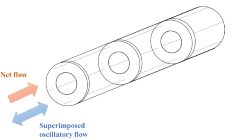
Continuous oscillatory baffled reactors (COBRs) have been proven to globally intensify processes, leading to processes that use less energy and produce fewer wastes (Phan et al., 2011; Reis et al., 2006). An example of a COBR with single orifice baffles is shown in Figure 1. Due to the combination of a net flow and pulsations, and the interaction of this flow with baffles, these reactors offer interesting advantages over traditional mixing processes performed in stirred tanks, such effective mixing, mass and heat transfer in laminar and transitional flow (Mackley and Stonestreet, 1995; Ni et al., 2000; Stephens and Mackley, 2002), as well as plug flow with long residence times in compact geometries (i.e. reduced length-to-diameter ratio tube) (Harvey et al., 2001). These characteristics have been shown to be beneficial for liquid-liquid reactions (Lobry et al., 2014; Mazubert et al., 2015), polymerisation processes (Ni et al., 2001, 1999) and crystallization processes (Ni et al., 2004; Lawton et al., 2009; Agnew et al., 2017), amongst others.
Figure 1. Schematic of a continuous oscillatory baffled reactor with a standard single orifice plate geometry.
Continuous oscillatory flow in COBRs is characterized by different dimensionless numbers, such as the net flow Reynolds number (!"#$%), oscillatory Reynolds number (!"-), Strouhal number (;<), and velocity ratio (=), which are defined as:
!"#$% = >?#$%@ A (1) !"-=2BCD-@ A (2)
3 ;< = @ 4BD -(3) = = !" -!"#$% (4)
In !"-, the characteristic velocity is the maximum oscillatory velocity and has been used to describe the intensity of mixing in the COBR. Stonestreet and Van Der Veeken (1999) identified different flow regimes: for !"-< 250 the flow is essentially 2-dimensional and axi-symmetric with low mixing
intensity; for !"- > 250 the flow becomes 3-dimensional and mixing is more intense; finally, when
!"-> 2000, the flow is fully turbulent. The Strouhal number measures the effective eddy propagation
with relation to the tube diameter. Higher values of ;< will promote the propagation of the eddies into the next baffle (Ahmed et al., 2017). The most common range of the Strouhal number used in the literature is 0.15 < ;< < 4 (Abbott et al., 2012). However, this may not necessarily be the best operating range for processes, e.g. Mazubert et al. (2014) observed a decrease in the conversion of waste cooking oil into methyl esters for ;< > 0.1. The velocity ratio, ψ, describes the relationship between the oscillatory and net flow. It is typically recommended to operate at a velocity ratio greater than 1 to ensure that the oscillatory flow dominates the superimposed net flow (Stonestreet and Van Der Veeken, 1999). This ratio has been largely used to describe plug flow behaviour in the COBR.
In industrial processes, one important parameter to be considered is the energy dissipation rate or power density, since it influences mixing performance, mass and heat transfer, and scale-up guidelines. The energy dissipation rate in oscillatory flows can be characterised by the time-averaged power consumption over an oscillation period divided by the volume of the fluid. Experimentally, power density is determined by pressure drop measurements. In practice, pressure transducers are most often installed in the pipes upstream and downstream of the COBR, thereby encompassing fittings, bends and valves and hence making it difficult to determine the energy dissipation rate in the COBR alone. As a result, most of the studies on power dissipation in COBRs available in the literature employ empirical models, and only more recently CFD simulation. CFD is an attractive tool for this type of analysis since it allows the impact of the exact geometry on power consumption to be assessed without relying on any adjustable parameters, as is the case in empirical models. However, there are different ways to calculate power dissipation using CFD, including the volume integral of viscous dissipation (in laminar flow) or turbulence energy dissipation rate (in turbulent flow) and mechanical energy balances, and the computational ease and accuracy of each method may differ.
There are two models reported in the literature for estimating power density in pulsed batch columns and in oscillatory flow in tubes with no net flow: the quasi-steady flow model, QSM (Jealous and Johnson, 1955) and the eddy enhancement model, EEM (Baird and Stonestreet, 1995). These models, which assume high oscillatory velocities and a turbulent flow regime, are the only ones that have been employed for estimating power dissipation in COBRs.
4 The quasi-steady flow model (QSM) given by equation (5), postulates that the instantaneous pressure drop in an oscillation period is the same as the pressure drop that would be achieved in steady-state flow with the same velocity. The model is based on the standard pressure drop relation across a simple orifice. 1 2 = 2>H(ID-)J(1 K⁄ L− 1) 3BMNLO (5) This model has shown to be valid for high oscillation amplitudes D- (5-30 mm) and low oscillation frequencies C (0.5-2 Hz). In turbulent flow, the orifice discharge coefficient (MN) varies between 0.6 and 0.7 for simple orifices with sharp edges. However, at low Re, it is know that this coefficient is proportional to √!" and varies with the ratio of reactor diameter to orifice diameter, D/d (Johansen, 1930; Liu et al., 2001). Thus, this limits the application of the model to OBRs with orifice baffles and specific flow conditions. The QSM also assumes that there is no pressure recovery due to the short distance between orifice baffles. This assumption has been studied recently by Jimeno et al. (2018) who however claim that some pressure recovery does take place when the baffle spacing is 1.5D or greater.
The eddy enhancement model (EEM) is based on acoustic principles and the concept of eddy viscosity (Baird and Stonestreet, 1995). The model was developed considering the acoustic resistance of a single orifice plate, and by replacing the kinematic viscosity with the eddy kinematic viscosity at high Reynolds number. This model, given by equation (6), has been shown to be valid for low oscillation amplitudes D- (1-5 mm) and high frequencies C (3-14 Hz) values, which is the opposite to the QSM. It
also includes a mixing length (Q), which is an adjustable parameter corresponding to the average travel distance of turbulent eddies and is expected to be of the same order of the reactor diameter.
1 2 = 1.5>IJD -LQ KQR (6) In addition to the empirical nature of the mixing length l, which is dependent on reactor geometry, Reis et al. (2004) reported that it is also dependent on oscillation amplitude. This again limits the use of this model.
It is also pointed out that both models were developed for pulsed flow in tubes and columns without a net flow (i.e. equivalent to batch OBRs) and that they have been used to compare performances between classic stirred-tank reactors and OBR in different applications, as bioprocess and crystallization (Abbott et al., 2014; Ni et al., 2004). However, there is a very limited number of fundamental studies of energy dissipation rate in COBRs, therefore impeding the validation of these models. To date, only two studies have been carried out on this subject. Mackley and Stonestreet (1995) used a correction factor (given by equation (7)) in the QSM that takes into account the power density provided by the net flow. However, the physical meaning behind this correction factor remains unclear, making it difficult to use.
S = T1 + 4 V !" -B!"#W J X Y J Z (7)
5 Recently, Jimeno et al. (2018) performed CFD simulations of turbulent flow in a COBR with smooth constrictions and determined the power density via the pressure drop across the reactor for different oscillatory conditions. The results were compared with the values obtained using the QSM and the EEM. They found that the QSM over-estimates power density due to inappropriate values of geometrical parameters, whilst the EEM provides better agreement. Both models were then modified by adjusting the geometrical parameters (e.g. nx, C
D) and proposing an empirical correlation for mixing length, as
given in equations (8) and (9). The modified models predict similar power densities for a wide range of operating conditions in turbulent and are in good agreement with the authors’ CFD simulations of continuous flow in the COBR. Nevertheless, these models still include adjustable parameters based on reactor geometry, so it is expected that the values of these parameters would need to be modified again if the reactor geometry – in particular the baffle design – is altered.
1 2 = 2>H[.\(ID -)J]1 KZ L− 1^ 3BMNL_2 `Z a (8) 1 2 = 1.5H[.\>IJD -LQ∗ K_2 `Z a (9) Q∗= 0.002 bKL c BD-d [.e\ (10)
This work uses CFD simulation to compute power consumption in a NiTech® COBR with smooth constrictions for a range of net flow and oscillatory Reynolds numbers (!"#$% = 6 − 27 / !"-= 24 −
96). In particular, it explores two different ways to calculate power consumption – via viscous energy dissipation and using a mechanical energy balance, which are generic and therefore independent of COBR geometry – and evaluates them in terms of computational ease and accuracy. The range of operating conditions covered in the study complements the data recently obtained by Jimeno et al. (2018) and allows the validity of the QSM revised by these authors to be assessed.
2. Power dissipation characterization
Power dissipation is a key parameter for comparing the performance of different COBR geometries and operating conditions. In the laminar flow regime, the power dissipation can be calculated by the volume integral of the viscous dissipation:
1fN = g AΦic2 (11)
where Φi is the viscous dissipation function, which represents the energy loss per unit time and volume
6 Φi = 2 jV k?l kDW L + mk?n kop L + Vk?q krW L s + tmk?n kD p + V k?l koWu L + tVk?q koW + m k?n kr pu L + tVk?l kr W + V k?q kDWu L (12) Alternately, viscous dissipation can be evaluated using a mechanical energy balance. Assuming incompressible flow and zero velocity at the wall v = w, and applying Gauss's theorem, integration of the mechanical energy conservation equation over the fluid volume then gives:
1xy = − m c c<z 1 2>?Lc2 . f + z ({| ∙ v) c; . ~ + z 1 2>?L(v ∙ |) c; . ~ p = z AΦi c2 . f (13)
where 1xy refers to the power dissipation obtained via the mechanical energy equation, Term 1 is the
rate of increase of kinetic energy in the system, Term 2 is the work done by pressure on the fluid and Term 3 is the rate of addition of kinetic energy by convection into the system. In periodic motion, Term 1 is equal to zero over a flow cycle. Term 3 in equal to zero when the flow domain is unchanging with time and has an inlet (;Y) and outlet (;L) with the same area, ;.
The average power dissipation in the COBR has been calculated by taking the time average of equations (11) and (13) over an oscillation cycle, .
1fN 7-%ÄÅ = 1 z 1fN c< 7 [ (14) 1xy 7-%ÄÅ = 1 z 1xy c< 7 [ (15)
3. Numerical method
3.1. Geometry and operating conditions
The geometry studied is the NiTech® COBR, which is a single orifice baffled reactor with smooth constrictions, as shown in Figure 2(a). The COBR tube has a diameter (@) of 15 mm with 7.5 mm diameter orifices (c); the distance between orifices (or inter-baffle distance), QR, is 16.9 mm. The model test section comprised a tube of length (O) 144.5 mm and five orifices. A smooth reduction at the orifices was modelled to best represent the real geometry of the NiTech® glass COBR, as shown in Figure 2(b). The fluid considered in these simulations is a single-phase fluid with density > = 997 kg/m3 and dynamic viscosity A = 2×10⁻² Pa.s. Isothermal conditions were assumed. Table 1 lists the conditions used to study the interaction between the oscillatory conditions (frequency and amplitude) and net flow, and their influence on the power dissipation. The oscillatory frequency was set at between 1 Hz and
Term 2
7 2 Hz and the oscillatory amplitude was either 5 mm or 10 mm (i.e. 0.3QR–0.6QR). These values of amplitude fall in the optimal operational range of amplitudes described in previous studies (Brunold et al., 1989; Gough et al., 1997; Soufi et al., 2017). The net flow and oscillatory Reynolds numbers corresponding to these conditions were in the ranges 6–27 and 24–96, respectively, ensuring axi-symmetrical laminar flow since it is well below the transition to chaotic flow, i.e. for oscillatory Reynolds numbers less than 250 (Stonestreet and Van Der Veeken, 1999; Zheng et al., 2007). These flow conditions have enabled the COBR to be modelled as a thin wedge with symmetry boundary conditions on the front and back faces, which computational times to be reduced drastically. A no-slip boundary condition was applied to the inner walls of the reactor and the area-averaged gauge pressure was set to 0 Pa at the outlet.
(a)
(b)
Figure 2: (a) Photograph of the NiTech® COBR and (b) the geometry of the COBR simulated by CFD.
The numerical simulations of the flow in the COBR have been performed using the commercial package ANSYS CFX 18.2, which applies a finite volume discretization based on a coupled solver to solve the Navier-Stokes equations.
For incompressible, laminar, Newtonian flow, the transient Navier-Stokes equations for mass and momentum conservation are:
∇ ∙ v = 0 (16)
k(>v)
k< + ∇ ∙ (>v ⊗ v) = −∇{ + ∇ ∙ Ñ
(17) The boundary condition at the inlet of the COBR was described by a time-dependent velocity profile:
8 ? Ö#= 2?Ü V1 − ]á
!^
L
W (18)
where á is the radial position, á = (oL+ rL)YZL, and ! is the radius of the reactor and the mean velocity,
?Ü, is the sum of the velocity of the net flow and the oscillatory flow given by:
?Ü = ?#$% + 2BCD[âäH(2BC<) (19)
The convective terms were discretized using a second order bounded scheme and the second order backward Euler transient scheme was applied. Time steps were chosen to ensure the Courant-Friedrichs-Levy condition of convergence Mã < 1 and such that the results were time-step independent, as detailed in Section 3.4. Simulations were considered to be converged when the normalized residuals fell below 10–6.
Table 1: Simulation conditions proposed.
Case å (l h-1) ç (Hz) é è (mm) êë|ëí êëè Ψ 1 22.8 1 5 27 24 0.9 2 22.8 1.5 5 27 36 1.3 3 22.8 2 5 27 48 1.8 4 22.8 1 10 27 48 1.8 5 22.8 1.5 10 27 72 2.7 6 22.8 1.75 10 27 84 3.1 7 22.8 2 10 27 96 3.6 8 5.1 1 5 6 24 4.0 9 5.1 1.5 5 6 36 6.0 10 5.1 2 5 6 48 8.0 11 5.1 1 10 6 48 8.0 12 5.1 1.5 10 6 72 12.0 13 5.1 1.75 10 6 84 14.0 14 5.1 2 10 6 96 16.0
3.2. Meshing
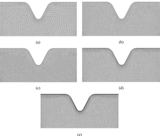
A tetrahedral mesh with inflation layers was used in all cases. The body size of the mesh and the number of inflation layers were chosen such that the results were independent of these parameters, as detailed in Section 3.4. An example image of the mesh is presented in Figure 3.
9
Figure 3: Example of tetrahedral mesh and inflation layers employed.
To ensure the numerical results are independent of the mesh density and time step, a detailed sensitivity analysis was carried out by studying the effect of different mesh sizes, inflation layer parameters and time steps on the results. The axial velocity, pressure and power dissipation were calculated and compared at the monitor points and lines shown in Figure 4, as well as the total power dissipation in one unit cell. !"-= 96 and !"#$% = 27 were used for all mesh density and time step studies, giving high axial velocity and a fast change of flow direction, which typically require a finer mesh. Details of all studied meshes and time steps are summarized in Table 2.
The simulations were run for several oscillation periods until the difference between the axial velocities and pressure values at different monitor points and lines from one oscillatory cycle to the next were small enough to be considered negligible. Once this was achieved, it was considered that a pseudo-steady state was reached and the performance characterization of the COBR was then conducted.
To minimize the effect of flow upstream and downstream of the baffles, the power dissipation was calculated using equations (14) and (15) in a single unit of the COBR delimited by lines L1 and L2 in Figure 4.
Figure 4: Locations of the monitor points and lines. M0: tube centerline, 8.45 mm upstream of the first orifice. M1 & L1: tube centerline, 8.45 mm upstream of the third orifice. M2: tube centerline, in the third orifice of the geometry. M3 & L2: tube centerline, at 8.45 mm downstream of the third orifice.
10 In order to evaluate mesh independency, the relative differences between data were calculated using the mean absolute deviation percent (MADP):
MADP = ∑ |`%− ô%| ö %õY ∑ö |ô%| %õY × 100 (20)
where `% is the actual value and ô% is the forecast value, both at time <. The results obtained with the finer mesh or smaller time step were used as ô% in the determination of relative error and values obtained
with the coarser mesh were used for `%. This method prevents having extremely large relative differences if ô% is close to or equal to zero, which occurs with other methods, such as the mean percentage error (MPE) or mean absolute percentage error (MAPE).
To study the effect of body mesh size, number of inflation layers and time step on the numerical results, five different meshes and three different time steps were chosen as described in Table 2. Examples of the studied meshes are shown in Figure 5.
(a) (b)
(c) (d)
(e)
Figure 5: Images of the meshes used for the mesh and time step independency study: (a) Mesh 1, (b) Mesh 2, (c) Mesh 3, (d) Mesh 4, (e) Mesh 5.
11
Table 2: Characteristics of different meshes used for the mesh and time step independency study.
Mesh Time-step Mesh 1 1 ms Mesh 2 1 ms Mesh 3 1 ms Mesh 4 1 ms Mesh 5 1 ms Mesh 4 2 ms Mesh 4 0.5 ms Max. face size (mm) 0.5 0.35 0.25 0.35 0.35 0.35 0.35
Max. thickness of
inflation layers (mm) 1
No. inflation layers 8 8 8 16 24 16 15
Growth rate 1.1
Total no. elements 150 165 337 873 719 957 433 986 528 703 433 986 433 986
∆" (s) 0.001 0.001 0.001 0.001 0.001 0.002 0.0005 #$ (mm) 10 % (Hz) 2 & (s) 0.5 ' = & ∆"⁄ 500 500 500 500 500 250 1000 * (Pa.s) 2 × 10⁻² +,-" (m/s) 3.59 × 10⁻² +/0# (m/s) 1.63 × 10⁻¹ 1-$ 96 1-,-" 27 2 3.6
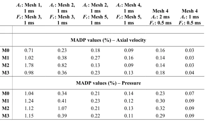
12 Table 3 presents the effect of the body mesh size, inflation layers and time step on the axial velocity and pressure values using the MADP. The axial velocity and pressure tracked at the monitor points show excellent mesh independency for the Mesh 2 (330 000 elements) with MADP values close to 1% with respect to the solution using Mesh 3 (720 000 elements). Between Mesh 2, 4 and 5, the MADP values (below 1%) show that the axial velocity and pressure are already independent of the number of inflation layers with Mesh 2 (8 inflation layers).
Table 3: Quantification of the effect of body mesh, inflation layers and time step on the axial velocity and pressure at different monitor points (M0-M3) with the MADP.
At : Mesh 1, 1 ms Ft : Mesh 3, 1 ms At : Mesh 2, 1 ms Ft : Mesh 3, 1 ms At : Mesh 2, 1 ms Ft : Mesh 5, 1 ms At : Mesh 4, 1 ms Ft : Mesh 5, 1 ms Mesh 4 At : 2 ms Ft : 0.5 ms Mesh 4 At : 1 ms Ft : 0.5 ms
MADP values (%) – Axial velocity
M0 0.71 0.23 0.18 0.09 0.16 0.03
M1 1.02 0.38 0.27 0.16 0.14 0.03
M2 1.78 0.82 0.13 0.09 0.14 0.03
M3 0.98 0.36 0.23 0.13 0.18 0.04
MADP values (%) – Pressure
M0 1.04 0.34 0.21 0.14 0.23 0.07
M1 1.24 0.41 0.23 0.12 0.30 0.09
M2 1.12 1.07 0.21 0.13 0.32 0.09
M3 1.15 0.39 0.22 0.11 0.29 0.09
The values of power dissipation calculated using equations (14) and (15), and the MADP values are presented in Table 4. An increase in body mesh density from Mesh 1 to Mesh 2 and Mesh 3 decreases the MADP of power dissipation calculated by both methods to less than 1% for !"# and !%&, and therefore shows mesh independency with Mesh 2. However, it is important to point out that the difference in power dissipation calculated by both methods !"# and !%& is still significant, being approximately 6% for the finest mesh (Mesh 3). This suggests that the resolution of the flow close to the wall is important for an accurate prediction of power dissipation.
The influence of the near-wall resolution (via the number of inflation layers) on the power dissipation can be seen in Table 4 by comparing results for Meshes 2, 4 and 5. The difference in !"#
obtained with 16 and 24 inflation layers is very small, therefore demonstrating mesh independency for !"# with 16 inflation layers (Mesh 4). The values of !%& on the other hand show that !%& is already mesh independent with just 8 inflation layers (Mesh 2). The values of !%& are higher than those of !"# and the latter increases towards the former when the number of inflation layers increases. This suggests
13 that !"# may be under predicted and it would be expected that the value of !"# should reach the value calculated by the mechanical energy balance if the mesh is further refined near the walls. However, only a slight increase in !"# is observed when the number of inflation layers is increased from 16 to 24. This means that an extremely large number of inflation layers would be required to reach the value of !%&, thereby increasing the simulation times and computational costs prohibitively.
Table 4: Influence of the body mesh, inflation layers, time step and power calculation method on power dissipation and MADP values.
Mesh 1, 1 ms Mesh 2, 1 ms Mesh 3, 1 ms
MADP values (%) At : Mesh 1, 1 ms Ft : Mesh 3, 1ms At : Mesh 2, 1 ms Ft : Mesh 3, 1 ms '() *+,-. (W) 3.51 × 10⁻⁵ 3.58 × 10⁻⁵ 3.61 × 10⁻⁵ 2.77 0.83 '/0 *+,-. (W) 3.90 × 10⁻⁵ 3.85 × 10⁻⁵ 3.83 × 10⁻⁵ 1.83 0.52
Mesh 2, 1 ms Mesh 4, 1 ms Mesh 5, 1ms
At : Mesh 2, 1 ms Ft : Mesh 5, 1 ms At : Mesh 4, 1 ms Ft : Mesh 5, 1 ms '() *+,-. (W) 3.58 × 10⁻⁵ 3.66 × 10⁻⁵ 3.68 × 10⁻⁵ 2.71 0.54 '/0 *+,-. (W) 3.85 × 10⁻⁵ 3.86 × 10⁻⁵ 3.85 × 10⁻⁵ 0.00 0.26
Mesh 4, 2 ms Mesh 4, 1 ms Mesh 4, 0.5 ms
At : Mesh 4, 2 ms Ft : Mesh 4, 0.5 ms At : Mesh 4, 1 ms Ft : Mesh 4, 0.5 ms '() *+,-. (W) 3.66 × 10⁻⁵ 3.66 × 10⁻⁵ 3.67 × 10⁻⁵ 0.27 0.27 '/0 *+,-. (W) 3.78 × 10⁻⁵ 3.86 × 10⁻⁵ 3.89 × 10⁻⁵ 2.83 0.77
Mesh 4 (0.35 mm body mesh size and 16 inflation layers) was used to study the influence of the time step, since it showed mesh independency for power dissipation. Three values of time steps – 0.5 ms, 1 ms and 2 ms – were used to evaluate mesh independency. Table 3 shows that both the axial velocity and pressure are independent of time step for a value of 2 ms, with MADP values lower than 1%. In Table 4, it can be noticed that !"# is already time step independent at 2 ms, whilst !%& only becomes time step independent at 1 ms. A time step of 1 ms is therefore considered as the minimum time step required for solution independency.
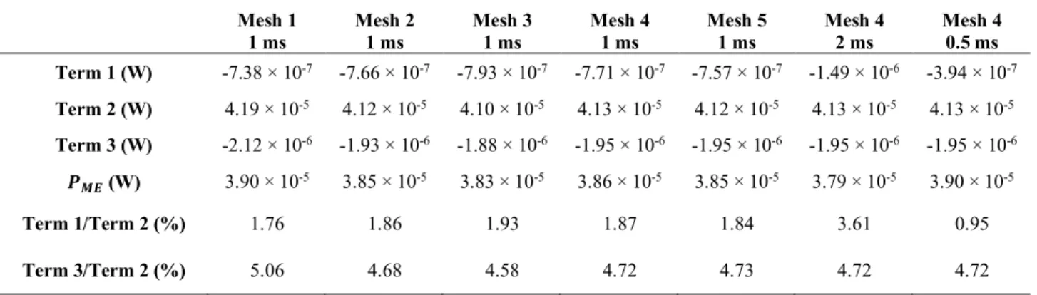
3.3. Implications for the calculation of !
%&Table 5 presents the time-averaged value of !%& over one oscillation cycle, as well as the time-averaged values of each term given in equation (13). Term 1 is shown to be sensitive to the time step, while Term 3 is sensitive to the mesh size. Term 1 decreases as the time step decreases, whilst Term 3 decreases as the mesh size is reduced. The influence of the number of inflation layer does not show any
14 remarkable influence over the value of any of the three terms of the !%& equation. Despite these reductions, it can be seen that the values of Terms 1 and 3 are ten times smaller than that of Term 2; however, they do not reach a zero-value due to finite errors arising from discretisation of the equations. Terms 1 and 3 represent between 1-4% and 4-5% of the total power dissipation, respectively. As explained in Section 2.1, Terms 1 and 2 should be zero in the current case such that the power dissipation is only dependent on the work done by pressure on the fluid. Hence, to avoid this numerical error, !%& is calculated using only the value of Term 2 in the rest of the study.
Table 5: Contribution of the individual terms of equation (13) on power dissipation !%&. Mesh 1 1 ms Mesh 2 1 ms Mesh 3 1 ms Mesh 4 1 ms Mesh 5 1 ms Mesh 4 2 ms Mesh 4 0.5 ms Term 1 (W) -7.38 × 10⁻⁷ -7.66 × 10⁻⁷ -7.93 × 10⁻⁷ -7.71 × 10⁻⁷ -7.57 × 10⁻⁷ -1.49 × 10⁻⁶ -3.94 × 10⁻⁷ Term 2 (W) 4.19 × 10⁻⁵ 4.12 × 10⁻⁵ 4.10 × 10⁻⁵ 4.13 × 10⁻⁵ 4.12 × 10⁻⁵ 4.13 × 10⁻⁵ 4.13 × 10⁻⁵ Term 3 (W) -2.12 × 10⁻⁶ -1.93 × 10⁻⁶ -1.88 × 10⁻⁶ -1.95 × 10⁻⁶ -1.95 × 10⁻⁶ -1.95 × 10⁻⁶ -1.95 × 10⁻⁶ '/0 (W) 3.90 × 10⁻⁵ 3.85 × 10⁻⁵ 3.83 × 10⁻⁵ 3.86 × 10⁻⁵ 3.85 × 10⁻⁵ 3.79 × 10⁻⁵ 3.90 × 10⁻⁵ Term 1/Term 2 (%) 1.76 1.86 1.93 1.87 1.84 3.61 0.95 Term 3/Term 2 (%) 5.06 4.68 4.58 4.72 4.73 4.72 4.72
4. Results and discussion
Figure 6 shows the time-averaged power density as a function of oscillatory Reynolds number for all operating conditions given in Table 1. As expected, the power density increases with an increase in the oscillatory intensity, i.e. f.xo. The effects of frequency and amplitude at constant oscillatory intensity
(123 = 48) but different net Reynolds numbers are examined by comparing Cases 3 & 4 (12789 = 27,
ψ = 1.8) and Cases 10 & 11 (12789 = 6, ψ = 8). For both Renet, slightly higher values of power density
were obtained when a higher frequency and a lower amplitude are combined. This may be explained by the fact that the average power dissipation in oscillatory systems is determined by pressure drop, which includes the contribution of both inertial and frictional forces (Jealous and Johnson, 1955). The inertial term involves acceleration, which in oscillatory flow is equal to =3(2?@)Bsin(2?@F). Since frequency
is squared in this relationship, higher values of average power density are obtained when higher frequencies are used for a constant oscillatory Reynolds number.
The influence of net flow can also be studied in Figure 6 and it can be seen that for a given Reo, as
the net flow increases (i.e. the oscillatory to net velocity ratio ψ decreases), power density also increases. For high values of ψ, the contribution of the net flow becomes insignificant, because the intensity of the oscillatory flow greatly exceeds the contribution of the net flow. This trend can be observed explicitly in Figure 7. Whilst at 123 = 24, an increase in the velocity ratio from 1 to 4 (by decreasing the net flow), reduces the power density by 71%. At 123 = 96, increasing the velocity ratio from 4 to 16 only
15 results in a reduction of power density by 12%. This result is of interest when operating COBRs in the recommended range of velocity ratios to ensure plug flow operation, i.e. 2 < ψ < 6 (Stonestreet and Harvey, 2002); in such cases, it clearly appears to be important to take into account the effect of the net flow in the average power dissipation.
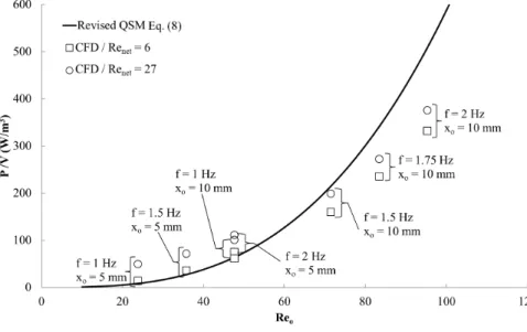
Figure 6: Power density as function of 123.
Figure 7: Power density as a function of velocity ratio (ψ).
The power density determined by equation (13) was initially compared with the power density calculated using the quasi-steady flow model given by equation (5), since the latter is recommended for high amplitudes (5 < =3< 30 mm) and low frequencies (0.5 < @ < 2 Hz). To include the contribution of the net flow in the power density, the correction coefficient from equation (7) was also used. For all cases, the power density was overestimated when equations (5) and (7) were used, with extremely high MADP values of 165% for H#= 0.7, and 261% for H#= 0.6. A similar result has been recently reported by Jimeno et al. (2018) for the same NiTech® COBR geometry used here and was explained
16 by the power law dependency on the number of baffles cells, as well as the use of an inappropriate value of the discharge coefficient H# for the smooth geometry of the orifice baffles. Jimeno et al. (2018) hence
proposed the revised QSM (equation (8)) to better estimate the power density. Figure 6 also compares the power density obtained with the values calculated using the revised quasi-steady flow model (equation 8). The differences between the current results with the revised QSM predictions present a MADP of 35.7%, with a better agreement at lower 12789 and 123 but still poor agreement at higher 123. It can also be seen that the influence of net flow is not taken into account in the original model.
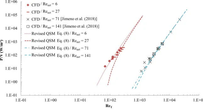
Figure 8 compares the power density of the revised quasi-steady flow model (equation 8) with the current simulation results as a function of 12K as defined by Jimeno et al. (2018). This total Reynolds number takes into account the effect of the net flow and the geometry of the COBR and is defined as:
12K= (2?@=3+ M789)NO P Q R S (21) R = TU 3V9 TU (22)
TU3V9 is defined as 1.5O, and was proposed by Brunold et al. (1989) based on a qualitatively visual analysis of flow patterns. Even though this baffle spacing of 1.5O was considered ‘optimal’ and is now the most commonly used value in the literature, recent studies have demonstrated that the optimal baffle length depends on the process objective of interest (Soufi et al., 2017), making a single optimal value difficult to define for all applications and processes. For each set of data different curves can now be observed because the net flow is being taken into account in 12K and this is more consistent with the current results of the simulated power density. It appears that the model fits the simulated data slightly better at 12789 = 6 than at 12789 = 27, and this can be related to the velocity ratio ranges of each curve. The highest net Reynolds number curve (12789 = 27) presented the lowest values of ψ (1 < ψ < 3.6), which means a more significant influence of the net flow, however this is not taken into account in the determination of power density with the revised quasi-steady flow model. Power density as a function of 12K as predicted by the QSM is presented in Figure 8 and compared with the data of Jimeno et al.
(2018) and this work. Their COBR geometry is also a NiTech® single orifice baffled reactor with smooth constrictions, with a tube diameter of 15 mm, 7.5 mm diameter orifices and a distance between orifices of 23.5 mm. The shift between red and blue curves is due the nature of the fluid used: power density is higher at the same 12K when working with more viscous fluids. Since 12K is inversely proportional to the viscosity, the characteristic velocity needs to be increased in order to obtain the same 12K when working with more viscous fluids. The power density is directly proportional to the pressure drop of the system, which increases with increasing flow velocities and viscosity due to increased friction. This observation is in agreement with the work by González-Juárez et al., (2018). Figure 8 shows that for the same fluid and system, power density – as predicted by the model – is independent of 12789 only for relatively high 12K. For a specific fluid type and corresponding relatively low 12K,
17 plotting QSM as a function of 12K results in the prediction of different power densities depending on 12789. Jimeno et al. (2018) state that their revised quasi-steady flow model is valid in both OBRs (batch) and COBRs, claiming that the contribution of the net flow to the power dissipation is negligible when operating with velocity ratios between 6 and 150. However, the current results do not always corroborate this. Figure 7 shows the effect of the velocity ratio and the oscillatory Reynolds number on the power density. Whilst the data are scant, it appears that as the oscillatory Reynolds number increases, the impact of the velocity ratio on power density decreases. Indeed, for 123 = 96 power density decreases by 12% when the velocity ratio increases from 4 to 16, whilst for 123 = 24 it decreases by 71% when the velocity ratio increases from 1 to 4. However, it is also easily seen at a fixed velocity ratio, e.g. ψ = 4, the higher oscillatory Reynolds number results in significantly higher power density. Identifying a velocity ratio whereby the contribution of net flow to power dissipation is negligible does therefore not seem to be straightforward since it also depends on the oscillatory flow. As a result, the limits of validity of the revised QSM (where the contribution of the net flow to power density can be assumed negligible) remain unclear.
Figure 8: Power density as function of 12K.
Although previous studies in the literature have tried to correlated power density with the oscillatory Reynolds number (e.g. González-Juárez et al., 2018; Jimeno et al., 2018), for chemical engineering design, it is more useful to plot a dimensionless form of the dissipated mechanical energy as a function of Reynolds number such that the effect of fluid properties are eliminated; the resulting plot depends on system geometry only. Some common examples are the friction factor for the flow in pipes or the power number in stirred tanks. One common feature of these charts is that for a specific geometry, the dimensionless number representing energy dissipation is constant in fully-developed turbulent flow,
18 whilst it is inversely proportional to Reynolds number in laminar flow. In a similar manner, one can define a dimensionless power density (!/Z)∗ as:
\! Z]
∗
= (!/Z)O
N(2?@=3+ M789)^ (23)
Figure 9 presents the dimensionless power density for the NiTech® COBR from the current simulations and those conducted by Jimeno et al. (2018). The data are compared with dimensionless power density that has been predicted from the revised QSM. It can be seen that for 12K< 300, (!/Z)∗
from the simulations is proportional to (12K)ab and for 12
K > 1000, (!/Z)∗ is constant, as would be
expected. From these data, the power density constants for the NiTech® geometry in laminar flow and in turbulent flow are found to be:
(!/Z)∗= 330 12 K
⁄ for laminar flow (S = 0.25 / TU= 1.1O) (24)
(!/Z)∗= 1.92 for turbulent flow (S = 0.22 / T
U = 1.6O) (25)
Figure 9: Dimensionless power density as a function of 12K.
It can also be seen that whilst the revised QSM correctly predicts the constant value of (!/Z)∗ in
fully turbulent flow, it provides an unphysical representation of power density in the transitional and laminar flow regimes. The QSM is hence only useful for predicting power density in fully developed turbulent flow. However, it should be kept in mind that it may be difficult to reach turbulent flow in many applications either because the fluid viscosity is relatively high (e.g. liquid-liquid flows) or the net flow rates are lowered to increase residence times, therefore resulting in lower oscillatory velocities such that the velocity ratio is kept in a reasonable range. The power curve shown in Figure 9 is therefore a useful design tool for predicting power density and pressure drop in the NiTech® COBR over a range of
19 flow regimes. It is obvious that the development of similar curves for other COBR and baffle geometries would also be of significant use.
5. Conclusions
CFD simulations have been carried out to evaluate power density in a COBR with single orifice baffles for different operating conditions.
The calculation of power dissipation using the simplified mechanical energy balance equation is preferred over the viscous dissipation equation, since when using the latter method it is difficult to resolve without using extremely fine mesh near the walls and consequently very high computational resources. Determination of power dissipation via the mechanical energy balance enables an exact value to be obtained, providing that mesh independence is demonstrated, which is the case here.
Comparison of computed power dissipation with that predicted by empirical quasi-steady flow models found in the literature shows that these models are still not able to correctly predict the values for all operating conditions and in particular when the flow is not fully turbulent. Indeed, when the flow is not fully turbulent, the QSM provides an unphysical representation of power density. The operating conditions used to define the limits of validity of the QSM therefore appear to be more complex than merely high/low frequencies and amplitudes, and the velocity ratio. 123 and 12789 and the resulting
flow regime play a very important role. By plotting dimensionless power density as a function of Reynolds number based on the sum of both the oscillatory and net flow velocities, 12K, it has been demonstrated that dimensionless power dissipation is inversely proportional to 12K in laminar flow and constant in turbulent flow, as is the case for flow in pipes and stirred tanks.
6. Acknowledgements
The authors acknowledge the University of Sydney’s high performance computing cluster Artemis for providing High Performance Computing resources that have contributed to the research results reported in this paper, as well as the Mexican Council of Science and Technology (CONACYT México) and Toulouse INP for diverse funding.
20
7. References
Abbott, M.S.R., Harvey, A.P., Perez, G.V., Theodorou, M.K., 2012. Biological processing in oscillatory baffled reactors: operation, advantages and potential. Interface Focus 3, 20120036. https://doi.org/10.1098/rsfs.2012.0036
Abbott, M.S.R., Valente Perez, G., Harvey, A.P., Theodorou, M.K., 2014. Reduced power
consumption compared to a traditional stirred tank reactor (STR) for enzymatic saccharification of alpha-cellulose using oscillatory baffled reactor (OBR) technology. Chem. Eng. Res. Des. 92, 1969–1975. https://doi.org/10.1016/j.cherd.2014.01.020
Agnew, L.R., McGlone, T., Wheatcroft, H.P., Robertson, A., Parsons, A.R., Wilson, C.C., 2017. Continuous crystallization of paracetamol (acetaminophen) form II: selective access to a metastable solid form. Cryst. Growth Des. 17, 2418–2427.
https://doi.org/10.1021/acs.cgd.6b01831
Ahmed, S.M.R., Phan, A.N., Harvey, A.P., 2017. Scale-up of oscillatory helical baffled reactors based on residence time distribution. Chem. Eng. Technol. 40, 907–914.
https://doi.org/10.1002/ceat.201600480
Baird, M.H.I., Stonestreet, P., 1995. Energy dissipation in oscillatory flow within a baffled tube. Trans IChemE 73(A), 503–511.
Brunold, C.R.R., Hunns, J.C.B.C.B., Mackley, M.R.R., Thompson, J.W.W., 1989. Experimental observations on flow patterns and energy losses for oscillatory flow in ducts containing sharp edges. Chem. Eng. Sci. 44, 1227–1244. https://doi.org/10.1016/0009-2509(89)87022-8 González-Juárez, D., Herrero-Martín, R., Solano, J.P., 2018. Enhanced heat transfer and power
dissipation in oscillatory-flow tubes with circular-orifice baffles: a numerical study. Appl. Therm. Eng. 141, 494–502. https://doi.org/10.1016/j.applthermaleng.2018.05.115
Gough, P., Ni, X., Symes, K.C., 1997. Experimental flow visualisation in a modified pulsed baffled reactor. J. Chem. Technol. Biotechnol. 69, 321–328. https://doi.org/10.1002/(SICI)1097-4660(199707)69
Harvey, A.P., Mackley, M.R., Stonestreet, P., 2001. Operation and optimization of an oscillatory flow continuous reactor, in: Industrial and Engineering Chemistry Research. pp. 5371–5377.
https://doi.org/10.1021/ie0011223
Jealous, A.C., Johnson, H.F., 1955. Power requirements for pulse generation in pulse columns. Ind. Eng. Chem. 47, 1159–1166. https://doi.org/10.1021/ie50546a021
Jimeno, G., Lee, Y.C., Ni, X.-W.W., 2018. On the evaluation of power density models for oscillatory baffled reactors using CFD. Chem. Eng. Process. - Process Intensif. 134, 153–162.
https://doi.org/10.1016/J.CEP.2018.11.002
Johansen, F.C., 1930. Flow through pipe orifices at low reynolds numbers. Proc. R. Soc. A Math. Phys. Eng. Sci. 126, 231–245. https://doi.org/10.1098/rspa.1930.0004
21 pharmaceuticals using a continuous oscillatory baffled crystallizer. Org. Process Res. Dev. 13, 1357–1363. https://doi.org/10.1021/op900237x
Liu, S., Afacan, A., Masliyah, J.H., 2001. A new pressure drop model for flow-through orifice plates. Can. J. Chem. Eng. 79, 100–106. https://doi.org/10.1002/cjce.5450790115
Lobry, E., Lasuye, T., Gourdon, C., Xuereb, C., 2014. Liquid-liquid dispersion in a continuous oscillatory baffled reactor - application to suspension polymerization. Chem. Eng. J. 259, 505– 518. https://doi.org/10.1016/j.cej.2014.08.014
Mackley, M.R., Stonestreet, P., 1995. Heat Transfer and Associated Energy Dissipation for Oscillatory Flow in Baffled Tubes. Chem. Eng. Sci. 50, 2211–2224.
Mazubert, A., Aubin, J., Elgue, S., Poux, M., 2014. Intensification of waste cooking oil transformation by transesterification and esterification reactions in oscillatory baffled and microstructured reactors for biodiesel production. Green Process. Synth. 3, 419–429. https://doi.org/10.1515/gps-2014-0057
Mazubert, A., Crockatt, M., Poux, M., Aubin, J., Roelands, M., 2015. Reactor comparison for the esterification of fatty acids from waste cooking oil. Chem. Eng. Technol. 38, 2161–2169. https://doi.org/10.1002/ceat.201500138
Ni, X., Cosgrove, J.A., Arnott, A.D., Greated, C.A., Cumming, R.H., 2000. On the measurement of strain rate in an oscillatory baffled column using particle image velocimetry. Chem. Eng. Sci. 55, 3195–3208. https://doi.org/10.1016/S0009-2509(99)00577-1
Ni, X., Johnstone, J.C., Symes, K.C., Grey, B.D., Bennett, D.C., 2001. Suspension polymerization of acrylamide in an oscillatory baffled reactor: from drops to particles. AIChE J. 47, 1746–1757. https://doi.org/10.1002/aic.690470807
Ni, X., Zhang, Y., Mustafa, I., 1999. Correlation of polymer particle size with droplet size in suspension polymerisation of methylmethacrylate in a batch oscillatory-baffled reactor. Chem. Eng. Sci. 54, 841–850. https://doi.org/10.1016/S0009-2509(98)00279-6
Ni, X.W., Valentine, A., Liao, A., Sermage, S.B.C., Thomson, G.B., Roberts, K.J., 2004. On the crystal polymorphic forms of L-glutamic acid following temperature programmed crystallization in a batch oscillatory baffled crystallizer. Cryst. Growth Des. 4, 1129–1135.
https://doi.org/10.1021/cg049827l
Phan, A.N., Harvey, A., Lavender, J., 2011. Characterisation of fluid mixing in novel designs of mesoscale oscillatory baffled reactors operating at low flow rates (0.3-0.6ml/min). Chem. Eng. Process. Process Intensif. 50, 254–263. https://doi.org/10.1016/j.cep.2011.02.004
Reis, N., Gonç, C.N., Vicente, A.A., Teixeira, J.A., 2006. Proof-of-concept of a novel
micro-bioreactor for fast development of industrial bioprocesses. Biotechnol- ogy Bioeng. 95, 744–753. https://doi.org/10.1002/bit.21035
Reis, N., Vicente, A.A., Teixeira, J.A., Mackley, M.R., 2004. Residence times and mixing of a novel continuous oscillatory flow screening reactor. Chem. Eng. Sci. 59, 4967–4974.
22 https://doi.org/10.1016/j.ces.2004.09.013
Soufi, M.D., Ghobadian, B., Najafi, G., Mohammad Mousavi, S., Aubin, J., 2017. Optimization of methyl ester production from waste cooking oil in a batch tri-orifice oscillatory baffled reactor. Fuel Process. Technol. 167, 641–647. https://doi.org/10.1016/j.fuproc.2017.07.030
Stephens, G.., Mackley, M.., 2002. Heat transfer performance for batch oscillatory flow mixing. Exp. Therm. Fluid Sci. 25, 583–594. https://doi.org/10.1016/S0894-1777(01)00098-X
Stonestreet, P., Harvey, A.P.P., 2002. A mixing-based design methodology for continuous oscillatory flow reactors. Chem. Eng. Res. Des. 80, 31–44. https://doi.org/10.1205/026387602753393204 Stonestreet, P., Van Der Veeken, P.M.J., 1999. The effects of oscillatory flow and bulk flow
components on residence time distribution in baffled tube reactors. Chem. Eng. Res. Des. 77, 671–684. https://doi.org/10.1205/026387699526809
Zheng, M., Li, J., Mackley, M.R., Tao, J., Zhengjie, M., Tao, L.R.M., Zheng, M., Li, J., Mackley, M.R., Tao, J., 2007. The development of asymmetry for oscillatory flow within a tube containing sharp edge periodic baffles. Cit. Phys. Fluids 19. https://doi.org/10.1063/1.2799553͔
8. Nomenclature
e COBR cross-section area (m-2) e9 actual value at time F
f9 forecast value at time F
H# orifice discharge coefficient (-)
Hg Courant number, h ∆F ∆=j (-)
O COBR diameter (m)
k baffle orifice diameter (m)
@ oscillation frequency (Hz)
T mixing length (m)
T∗ mixing length proposed by Jimeno et al. (2018b) (m)
TU distance between baffles (m)
TU3V9 optimum distance between baffles (m)
l reactor length (m)
m number of baffles (-)
n normal vector (-)
o pressure (Pa)
! power dissipation (W)
!"# power dissipation calculated using the viscous dissipation equation (W) !%& power dissipation calculated using the mechanical energy equation (W)
23 (!/Z)∗ dimensionless power density (-)
1 radius of reactor (m)
12789 net flow Reynold number (-)
123 oscillatory Reynolds number (-)
12K total Reynolds number proposed by Jimeno et al. (2018b) (-)
p radial coordinate (m) q surface (m2) ∆F time step (s) F time (s) r oscillation period (s) Ms7 initial velocity (m s-1) M instantaneous velocity (m s-1) Mt mean velocity (m s-1) M789 net velocity (m s-1) Mu, Mv, Mw velocity components (m s-1) x velocity vector (m s-1) Z volume (m3) =3 oscillation amplitude (m) =, z, { cartesian coordinates (m) Greek symbols
S free baffle area |k Oj }B(-)
R optimal to use baffle spacing ratio (-)
P dynamic viscosity (Pa.s)
Φ dissipation function (s-2) N fluid density (kg m-3) τ theoretical residence time (s)
Å shear stress vector (Pa)
Ç velocity ratio (-)
É correction factor (-)
Ñ number of time steps in an oscillatory cycle (-) ω oscillation angular frequency (rad s-1)