The Timing of Elections in Federations : A Disciplining Device against Soft Budget Constraints ?

HAL Id: halshs-00492085

https://halshs.archives-ouvertes.fr/halshs-00492085

Submitted on 15 Jun 2010

HAL is a multi-disciplinary open access archive for the deposit and dissemination of

sci-L’archive ouverte pluridisciplinaire HAL, est destinée au dépôt et à la diffusion de documents

The Timing of Elections in Federations : A Disciplining

Device against Soft Budget Constraints ?

Karolina Kaiser, Emmanuelle Taugourdeau

To cite this version:

Karolina Kaiser, Emmanuelle Taugourdeau. The Timing of Elections in Federations : A Disciplining Device against Soft Budget Constraints ?. 2010. �halshs-00492085�

Documents de Travail du

Centre d’Economie de la Sorbonne

The Timing of Elections in Federations : A Disciplining Device against Soft Budget Constraints ?

Karolina KAISER, Emmanuelle TAUGOURDEAU

The Timing of Elections in Federations:

A Disciplining Device against Soft

Budget Constraints?

Karolina Kaiser

University of Munich

Emmanuelle Taugourdeau

CNRS, CES, Paris School of Economics

February 2010

For valuable comments and suggestions we would like to thank Andreas Hau‡er, Marie-Laure Breuillé, Basak Akbel, the participants of the 3rd IEB Workshop on Fiscal Federalism in Barcelona, the participants of the Soft Budget Constraint Workshop in Osaka, Japan, as well as the participants of the Research Seminar and the Public Economics Seminar at the Ludwigs-Maximilians-University Munich.

y_{University of Munich, Ludwigstr. 33/III, 80539 Munich, Germany. Tel: +49 89 2180 6781.}

Email: karolina.kaiser@lrz.uni-muenchen.de

z_{ENS Cachan, CES, Laplace 309, 61 avenue du president Wilson, 94235 Cachan Cedex,}

Abstract

We introduce political economics into the soft budget constraint problem by asking if the timing of elections has the potential to harden budget constraints. Speci…cally, we ask under which circumstances the soft budget constraint problem is worse - with synchronized elections, i.e. simultaneous central and regional o¢ ce terms, or with staggered elections, i.e. terms of o¢ ce that do not coincide. We …nd that stag-gered elections clearly improve …scal discipline at the local level as well as welfare.

Keywords: Soft Budget Constraints, Fiscal Federalism, Elections. JEL Classi…cation: D72, H77

Résumé

Dans cet article, nous introduisons des élements d’économie poli-tique dans un problème de contrainte budgétaire molle en étudiant si l’organisation simultanée ou décalée des éléctions nationales et locales a un impact sur la discipline budgétaire des gouvernements locaux. Nous montrons que des élections décalées permettent très clairement de dur-cir la contrainte budgétaire molle et améliorent le bien-être des agents de la fédération. Ce résultat s’explique par le fait que le gouvernement central bénéfécie d’une position de leadership en élections décalées qui permet de contenir le comportement opportuniste des gouvernements locaux.

Mots-clef: Contrainte Budgétaire Molle, Fédéralisme Fiscal, Elec-tions.

1

Introduction

Following (Rodden et al. , 2003), the soft budget constraint can be de…ned as “the situation when an entity (say, a province) can manipulate its access to funds in un-desirable ways”. Although it is widely acknowledged that soft budget constraints may cause ine¢ ciencies1 _{and should therefore be avoided, they are frequently}

ob-served (see Vigneault (2007) for an empirical survey). The recurrent emergence of soft budget constraints illustrates the di¢ culty of totally avoiding them and highlights the importance of better understanding the institutions which help to harden budget constraints.

To our best knowledge, very few papers have dealt with the characteristics of the political system2 _{although soft budget constraints are undoubtedly the results}

of interactions between two levels of government. In this context, the nature of the interactions may change depending on the electoral timetable. Since the soft budget constraint problem is a problem of commitment and therefore of timing, it might matter if regional and federal governments were elected at identical voting dates and decided at the same time on their revenues and expenditures for the upcoming term or if voting dates fall at di¤erent times. In our paper, we ask the question: does the timing of elections in federations matter for the soft budget constraint problem? In other words, in which system are budget constraints harder, with synchronized or with staggered subnational and national terms of o¢ ce? In practice, we observe either synchronized (Brazilia, Sweden or Denmark) or staggered (Canada, Germany or Australia) elections3 but the topic of concurrent vs. non-concurrent elections has received little attention for economic purposes although it has attracted the interest of political scientists4_{. The arguments in}

favor of one or the other system are usually based on cost considerations and on the question of voters’ confusion/motivation, but economic arguments are often missing in the debate. So, in contrast to the existing literature, we focus not on political but on economic variables such as the size of federal transfers, the amount of taxes raised and the magnitude of public and private consumption.

To answer our question we consider a simple model with T periods. A term of

1_{There are exceptions which show that soft budget contraints may diminish ine¢ ciencies}

arising from hard budget constraints (see Besfamille and Lockwood, 2008).

2_{One exception is Goodspeed (2002) who considers voting in his bailout model by including}

exogenous re-election probabilities for the central government. However, in contrast to our paper, he does not consider any interaction between the local and national elections.

3_{See Diamond, Larry, and Marc F. Plattner, eds. Electoral Systems and Democracy}

Balti-more: Johns Hopkins University Press pp 272 for more details.

4_{In particular, the political sciences analysis has investigated how the timing of elections}

interacts with di¤erent political variables such as the emergence of divided governments in pres-idential systems (Shugart, 1995), accountability of politicians (Samuels, 2004) or voter turnout (Hajnal and Lewis, 2003).

o¢ ce for both the federal and the local governments lasts for two periods. Local and federal o¢ ce terms can either be synchronized (SY) or staggered (ST). As a synchronized o¢ ce term regime we de…ne a model setup where elections and therefore the terms of o¢ ce for regional and federal governments coincide. On the contrary, a staggered o¢ ce term setting is a situation where regional elections take place just in the middle of the central government o¢ ce term. Therefore the terms of o¢ ce of old and new federal and regional governments overlap. Finally, we consider the situation of one region eligible for a federal discretionary grant on which the central government cannot commit. The federal government is inclined to allocate the grant due to lobbying, log-rolling practises or political purposes. By opposition to the mandatory grants which are rules-based obligations for the central government, discretionary grants are decided on a discretionary basis (some local jurisdictions may bene…t from them whereas others not). On the average of the OECD countries, the discretionary grants represent around 20% of the total amount of grants (Joumard et al. , 2005). In this article, we focus our analysis on the electoral system which diminishes the local incentives to manipulate the access to federal discretionary grants once a region is eligible. Indeed, as it has been observed in Finland where municipalities can apply for discretionary grants that are available during periods of exceptional circumstances, the system has in practice signi…cantly reduced the incentives for …scal discipline at the municipal level and “exceptional” grants are disbursed on an annual basis (Bergvall et al. , 2006). To reach our objective, we associate elections to a political program or an agenda which is implemented at the beginning of the o¢ ce term. In other words, policy variables are decided by the governments for the whole term when they enter o¢ ce.

Interestingly, we …nd that the staggered o¢ ce terms clearly dominate the syn-chronized o¢ ce terms. The intuition for this …nding is that in the staggered term setting the central government obtains a …rst mover advantage vis-à-vis the re-gional government entering next. This advantage is not at work for synchronized elections since bailouts are always chosen once all other economic variables are decided. With staggered elections, the …rst mover advantage enables the federal government to anticipate the strategic behavior of the next regional government, making it relatively easier to limit grants. Budget constraints are hardened by al-locating less funds to the second half of the o¢ ce term and using them to improve the allocation in the …rst half, where the old regional government can no longer strategically respond to actions of the central government because it has already made its tax and expenditure decisions in the previous period.

Our paper contributes to the literature of soft budget constraints by adding a political economy dimension to the debate. The soft budget constraint concept was introduced by Janos Kornai (1979, 1980) in the context of socialist enterprises

which got losses reimbursed by the state. Thereafter, this concept became perfectly suitable to analyze the consequences of decentralization and more precisely the in-teractions between several tiers of governments (for a literature overview see Kornai and al. 2003). Soft budget constraints are di¢ cult to avoid and are associated with major incentive problems regarding the accountability of regional governments in terms of …scal discipline. Therefore one important area of public economic re-search asked the question: how is the softness of budget constraints a¤ected by di¤erent characteristics of federations such as the size of regions (Wildasin, 1997 and Crivelli & Staal, 2006), the type of …scal equalization system or the intensity of tax competition (Qian and Roland, 1998 and Breuillé and al, 2006 , Koethen-buerger, 2007)? We go further along these lines by introducing political economic arguments generally developed in political science.

The remainder of the paper is organized as follows. Section 2 presents the basic model setup and Section 3 introduces a benchmark case, where a social planner makes e¢ cient taxation and expenditure decisions. In Section 4 we introduce a decentralized setup, where regional governments decide on regional taxation and expenditures and the central government is responsible for national public good provision. In addition, the central government has the opportunity to supplement regional public good provision through a bailout. In Section 4.1 we analyze syn-chronized terms of o¢ ce (SY) and in Section 4.2 staggered terms of o¢ ce (ST). Welfare is analyzed in Section 5 and Section 6 concludes.

2

Model

We consider a model of a federation with one region eligible for a discretionary grant and several regions which are not eligible for a grant5_{. The population of the}

eligible region is normalized to one, and the population of the non-eligible regions is normalized to N; N > 0, such that we have a total population of (N + 1) : Consumers At each date t; consumers in each region have an initial endowment of w and derive utility from a private good ct, a regional public good gt and a

national public good Gt. The payo¤s of consumers at a given date t are modeled

according to a log-linear utility function: ct+ gln gt+ Gln Gt.

Governments Governments are assumed to hold political power for one term of o¢ ce, which is divided into two sub-periods, the "post-electoral period" and the "pre-electoral period".

5_{We may assume that a proportion of the regions is eligible for a grant, but for symmetric}

eligible regions, it would not modify the results. To make the analysis clearer, we concentrate on the case of one eligible region.

Regional Governments At the beginning of each o¢ ce term, regional govern-ments choose their tax and expenditure policy. We act on the assumption that regional governments, when entering o¢ ce, …x their tax and expenditure policies in a political program that is valid for the whole o¢ ce term. In that sense, we consider that governments do not deviate from their agenda over time. This as-sumption enables us to link the elections to a political program and to concentrate our analysis on the timing of elections (staggered versus simultaneous). For reasons of simplicity, we abstract from distortionary taxation and allow regional govern-ments to choose a regional lump sum tax R

t as a revenue raising instrument. The

revenue collected can either be used for expenditures in the post-electoral period (st) or in the pre-electoral period (st+1). At the end of the term, the budget has

to be balanced: R

t = st+ st+1. While for non-eligible regions, regional public

consumption gt is solely …nanced by regional spending, the eligible region might

in addition receive a grant zt > 0 as a subsidy to regional expenditures, such that

the regional budget constraint is represented by gt = st+ zt;8t. The payo¤ of a

regional o¢ cial in one o¢ ce term is represented by the following utility function: ct+ gln gt+ Gln Gt+ ct+1+ gln gt+1+ Gln Gt+1 (1)

The separability of utility from regional, national and private consumption along with the quasi linearity assumption implies that optimal tax choices of the non-eligible regions are completely independent from tax choices of the eligible region.

Central government The central government has an own non-manipulable head tax C

t, which is …nanced from the initial endowment w of consumers and

is collected at the beginning of the central government’s o¢ ce term from each resident of the federation. The …xed level of the federal lump sum tax may be criticizable, but it enables us to concentrate our analysis on the local government behavior, which is the aim of the soft budget constraint analysis6. The total rev-enue (1 + N ) C

t can be used for post-electoral central government spending St or

pre-electoral spending St+1. In addition, in each period the central government

has to decide how to split up total spending among the national public good Gt

and a grant to the eligible region zt. Although particular grant programs may be

temporary, we argue that discretionary grants in general are given on a permanent basis to an eligible region. The central government has to balance the budget over the whole term, i.e. (1 + N ) C

t = St+ St+1, as well as in each period, i.e.

St= Gt+ zt;8t.

6_{It is possible to show that our results persist even with endogenous central government}

In order to make the problem interesting, we have to make a technical assump-tion regarding the exogenously given central government head tax. We assume that the revenue collected from the head tax is, on the one hand, large enough that a soft budget problem arises, and on the other hand, small enough that it is not possible that all activity of the eligible region is fully …nanced by central government grants in all periods, i.e. gt+ gt+1< zt+ zt+1 and zt> 0;8t. This

as-sumption is technically necessary to obtain an interior solution for the soft budget problem and to avoid corner solutions. The central government objective function is de…ned as:

ct+ gln gt+ (1 + N ) Gln Gt+ ct+1+ gln gt+1+ (1 + N ) Gln Gt+1 (2)

Since private and regional consumptions of the non-eligible regions are inde-pendent of the central government’s actions, they are disregarded in the central government’s objective function. However, this does not hold for the utility from the national public good, which is considered for all (1 + N ) inhabitants.

Timing In the synchronized o¢ ce terms set-up, we face an in…nitely repeated game, where at each date t + 2n; n 2 Z both a central and a regional government enter and stay for one o¢ ce term, consisting of a post-electoral and a pre-electoral period. In the staggered o¢ ce terms set-up there exists also an in…nitely repeated game, where at each date t + 2n; n 2 Z a central government and at each date (t + 1) +2n; n_{2 Z a regional government enter. Regional and central governments} decide when coming into o¢ ce on the intertemporal distribution of spending, i.e. st, st+1 and St, the level of R and St+1 being derived directly from the choices

of st, st+1 and St. The grants zt are chosen ex-post at each date t, after all other

…scal decisions have been made. The timing of each set-up is explained in more detail in the corresponding sections.

Before we move on to the construction of the synchronized and the staggered terms of o¢ ce regimes, we …rst establish a benchmark case, where a social planner maximizes the utility of all inhabitants over the whole o¢ ce term.

3

Social Planner

The social planner program serves as an e¢ ciency benchmark. The social planner solves the following problem,

max

st;st+1;zt;zt+1;St

ct+ gln gt+(1 + N ) Gln Gt+ ct+1+ gln gt+1+ (1 + N ) Gln Gt+1

(3) subject to the budget constraints:

ct = w Rt

C _c

t+1= w (4)

gt = st+ zt gt+1 = st+1+ zt+1 (5)

Gt = St zt Gt+1 = St+1 zt+1 (6)

and the budget balancing constraints:

R

t = st+ st+1 (1 + N ) C = St+ St+1 (7)

From the …rst order conditions w.r.t. st; st+1; zt; zt+1 we obtain a unique

solu-tion for regional public consumpsolu-tion gt= gt+1= g, for national public

consump-tion: Gt= Gt+1= (1 + N ) G, for the regional tax rate Rt = 2 g+ (1 + N ) G

(1 + N ) C and for private consumption ct = w 2 g+ (1 + N ) G + N C,

ct+1 = w: Through the budget balancing constraint Rt = st + st+1 the sum of

optimal regional spending is determined. However, the social planner is indi¤erent between spending the given regional tax revenue in period t or in period t + 1, because grants zt constitute a second instrument which allows the provision of an

optimal level of regional goods for each given level of spending 0 st Rt.

The sum of grants over both o¢ ce periods (zt+ zt+1) equals

(1 + N ) C ₂

G . Because the social planner accounts for all externalities

asso-ciated with the grants, this level of grants represents the ex-ante e¢ cient amount. If the central government could commit, it would pay this amount no matter what tax rate the eligible region chooses. However, in the subsequent set-ups we ana-lyze a situation where the central government cannot commit to an e¢ cient level of grants and tax policy is decentralized. In a simple one period model, these assumptions would lead to an ine¢ ciently low regional tax rate and to ine¢ ciently high grants for the eligible region. The intuition for this result is that the eligible region fails to account for the negative externalities associated with the grants. In the following section, we ask if this result persists in the same fashion for di¤erent o¢ ce term regimes (i.e. modi…ed timings).

RG CG t+3 t+2 t+1 t z_t+1 s_t,s_t+1 p ost-electoral period pre-electoral period z_t z_t+3 S_t,S_t+1 z_t+2 post-electoral period pre-electoral period s_t+2,s_t+3 S_t+2,S_t+3

Figure 1: Timing in the SY Regime

4

Decentralized Setup

In this section we introduce a decentralized set-up where regional governments choose the regional tax rate as well as regional expenditures whereas the central government chooses both the level of national expenditures and the amount of grants allocated to the eligible region.

4.1

Synchronized O¢ ce Terms

In the synchronized set-up, both a new regional and a new federal government enter into o¢ ce at the beginning of each term, and decide simultaneously on their expenditure policy. Additionally, at the end of each period, the central government decides on the level of grants. This sequence of events is repeated in…nitely7_.

Given that new o¢ cials enter at the beginning of each term, there are no strategic interactions across terms, and it is therefore su¢ cient to solve the game for one o¢ ce term.

The basic structure of this game is identical to a standard two-stage game with decentralized leadership of the regional government, which can be solved by backward induction.

7_{The ex-post grant yields an identical outcome as if an ex-ante e¢ cient grant is calculated}

At stage 2, the central government maximizes its objective function (2) w.r.t. ztand zt+1subject to the budget constraints (4) (7). The solution of this problem

is the following grant scheme: zt =

gSt (1 + N ) Gst

(1 + N ) _G+ _g 8t (8)

The central government is restricted in its actions in the sense that it is just allowed to increase regional revenue through grants, but not to reduce it, i.e. zt 0. Therefore the solution is an interior solution to a Kuhn-Tucker problem.

The grant function illustrates as well that the regional budget constraint is soft in the sense that it is optimal for the central government to compensate a reduced regional government spending with an increase of grants dzt

dst < 0. The transfer is

chosen such that the preferences of the central government on the distribution of public funds across the regional and the national public good are realized. As it is typical for Cobb-Douglas type utility functions, for each type of public good a constant share of revenue is spent. This becomes obvious when the grant (8) is plugged into regional and national public consumption: gt = _{(1+N )}g

G+ g (St+ st)

and Gt= _{(1+N )}(1+N ) G

G+ g (St+ st).

At stage 1, a Nash game between the central and the regional government is played when deciding on the expenditure policy for the following term of o¢ ce. While the regional government maximizes the utility of its own residents when maximizing (1) w.r.t. stand st+1, the central government cares for the utility of all

(1 + N ) residents by maximizing (2) w.r.t. St (and St+1 via the budget balancing

constraint (7)), subject to all budget constraints. We obtain the following response functions for the central and the regional governments:

St =

(st+1 st) + (1 + N ) C

2 (9)

st+ st+1 = g+ G 2 (1 + N )

C ₍₁₀₎

The best response function of the central government (9) shows the intertem-poral preferences of the central government. The adjustment of St according to

(9) insures that a constant fraction of funds is spent in the post-electoral period and in the pre-electoral period for each combination of st and st+1 chosen by the

regional government.

While the regional government’s best response function (10) is sensitive to the sum of central government spending St+ St+1 = (1 + N ) C, it is insensitive to

the intertemporal distribution of central government funds, i.e. to St.

and a ’level e¤ect’. The distribution e¤ect implies that the central government is decisive when it comes to the distribution of public funds through the stage 2 reaction function (8) as well as the stage 1 best response function (9). For the distribution of a given amount of funds between the regional and the national pub-lic good this is true because the central government has the …nal decision power by allocating grants ex-post8_{. However, the regional government is decisive with}

respect to the level e¤ect, i.e. for the level of total funds available for public con-sumption. This follows directly from the assumption that the central government has an exogenously given amount of tax revenue which it cannot manipulate. The regional government clearly prefers a lower amount of spending than the central government would do if it could choose the regional lump sum tax. By reducing its tax rate, the regional government bene…ts because it receives in turn grants whose costs are borne by all the residents of the federation. This negative inter-regional externality of the grant is characterized by a decrease of utility from national public consumption by the N outsiders, which the region does not take into account.

Solving for consumption variables yields the following results for private and public consumption: ct = w + N C 2 g + G ct+1= w gt = g g+ G g+ (1 + N ) G gt+1 = g g+ G g+ (1 + N ) G Gt= (1 + N ) G g+ G g+ (1 + N ) G Gt+1= (1 + N ) G g+ G g+ (1 + N ) G

If there were no residents outside the eligible region (N = 0), g+ G

g+(1+N ) G would

equal one and the preferences of the regional and the central governments would coincide with the social planner’s choices. N > 0 introduces interregional exter-nalities that let the regional and national public goods be underprovided since the negative externalities of raising too little revenue are not taken into account by the regional government. The following proposition summarizes the implications for the level of grants.

Proposition 1 A decentralized leadership with synchronized o¢ ce terms is asso-ciated with a higher level of grants than the social planner set-up.

8_{Note that there is no con‡ict of interest between the central and the regional governments}

on the intertemporal distribution of revenue because both governments prefer half of the funds in period t and half of the funds in period t+1.

Proof. In the social planner solution we have:

(zt+ zt+1)SP = (1 + N ) C 2 G

whereas for the synchronized terms of o¢ ce solution of the decentralized leadership we obtain: (zt+ zt+1)SY = (1 + N ) C 2 G g+ G (1 + N ) _G+ _g ! and clearly (zt+ zt+1)SP < (zt+ zt+1)SY

This result is in line with the existing literature (e.g Goodspeed (2002), Wildasin (1997)) and shows that the decentralized leadership, along with a lack of commitment of the federal government when deciding on the level of grants, creates a soft budget constraint mechanism (equa (8)).

4.2

Staggered O¢ ce Terms

The staggered o¢ ce terms set-up characterizes a federation with decentralized re-gional spending and taxation, where at each date t + 2n; n 2 Z a new central government enters o¢ ce and at each date (t + 1) + 2n; n 2 Z new regional gov-ernments come into o¢ ce. So, it di¤ers from the synchronized elections game by the feature that regional and central election dates do not coincide, but fall on di¤erent dates (see Figure 2). This has, …rst of all, implications for the sequence of events and outcomes.

The central government entering o¢ ce at date t has to take the regional spend-ing decision st as given because it has been chosen at date (t 1). So, the central

government’s position in the post-electoral period becomes weaker in the sense that its spending decision is no longer set simultaneously with the regional government. Instead, the regional government now obtains a …rst mover advantage. In contrast, the position of the central government at date (t + 1) is strengthened vis-à-vis the regional government as it can choose spending in the pre-electoral period St+1

be-fore the regional government chooses st+1. Similarly, the position of the regional

government in its post-electoral period is weakened and in its pre-electoral period strengthened. How does this a¤ect outcomes?

We solve this game by backward induction. Given that grants are always al-located ex-post after all other spending decisions have been made, the optimal grant scheme is identical to the grant scheme in the synchronized set-up (8). Once the grant scheme z (s ; S) ;_{8t is determined, it can be plugged into the public}

zt+1 St,St+1 St+2,St+3 zt+2 zt+3 st+1,st+2 st+3,st+4 post-electoral period pre-electoral period p ost-electoral period pre -electoral period t+3 t+2 t+1 t post-electo ral period pre-electoral p eriod zt post-electoral p eriod CG RG pre-electoral period

Figure 2: Timing in the ST regime.

consumption variables at all dates and the problem of the synchronized elections set up reduces to the choice of optimal spending for all dates. Although the max-imization problems of both governments remain the same, the budget constraints for private consumption (4) and the balanced budget constraint (7) change to:

ct= w C ct+1 = w Rt+1 (4a)

R

t+1 = st+1+ st+2 (1 + N ) C = St+ St+1 (7a)

This holds for all dates t + 2n; n 2 Z and (t + 1) + 2n; n 2 Z respectively. The other budget constraints stay unchanged.

We start with the calculation of the reaction functions of the regional govern-ments. The quasilinear structure of the utility function makes regional spending decisions for the post-electoral period, e.g. st+1 and the pre-electoral period, e.g.

st+2 independent from each other. While st+1 depends only on St+1 (chosen by

the central government which entered at date t), the choice of st+2 depends on the

anticipated behavior of the central government entering in the following period t + 2:Therefore, we determine in a …rst step the choice of st+1, then we determine

central government responses @St+2

@st+2 and in a third step, we solve for st+2.

When choosing st+1, the regional government maximizes the objective function:

with respect to st+1 taking into account the grant scheme (8) and the budget

constraints (4a) ; (5) ; (7) and (7a). We obtain the following …rst order condition:

g gt+1 @gt+1 @st+1 + G Gt+1 @Gt+1 @st+1 = 1 where g gt+1 @gt+1 @st+1 + G Gt+1 @Gt+1 @st+1 = g+ G St+1+ st+1 (12) The left hand side shows the marginal bene…ts of an increase in post-electoral spending, taking the responses @zt+1

@st+1 into account, whereas the right hand side

shows the marginal costs, which are constantly one due to the quasilinear consump-tion. Like in the synchronized elections setting, the regional government disregards the costs of forgone national public good consumption for the N citizens outside its territory. The response function derived from (12) : st+1 = g+ G St+1

illustrates that all attempts of the central government to increase public funds in period t + 1 are counteracted by a reduction of st+1.

Having obtained this response function, we can move on to solve the central government problem at date t, which is equal to maximizing (2) w.r.t. St,

tak-ing into account response functions (8), (12) as well as the budget constraints (4a) ; (5) ; (7) and (7a). The solution to this problem is characterized by the …rst order condition for St :

(1 + N ) _G Gt = 1 with Gt= (St+ st) (1 + N ) G g+ (1 + N ) G 8t + 2n; n 2 Z (13) The LHS of the condition represents the marginal bene…t of an increase of St

which equals the marginal bene…t of public consumption (the bene…ts of regional and national public consumption are equalized through the grant scheme). The RHS represents the marginal costs, which are equal to one. This results from the intertemporal link between Stand St+1through the balanced budget constraint and

the response behavior of the regional government @st+1

@St+1 = 1 according to (12).

Rearranging (13) to the explicit response function St = g+ (1 + N ) G st

makes it obvious that any attempt of the regional government to increase pub-lic funds for period t is fully counteracted by the central government through a decrease of St. The reaction functions (12) and (13) imply that the government

entering o¢ ce in a given period is decisive for the amount of public funds available in this period.

The central government response function (13) enables us to solve as a …nal step, the regional maximization problem w.r.t. st+2. The marginal costs of raising

st+2 are constantly equal to one, because of the quasilinear utility structure.

(13) it follows that @gt+2

@st+2 = 0 as well as

@Gt+2

@st+2 = 0. Therefore it is optimal for the

region to not spend any funds in its pre-electoral period (st+2 = 0) :

Solving for consumption variables yields the following results:

ct = w C ct+1 = w 2 g+ G + N + G (1 + N ) C (14) gt= g gt+1= g+ G g g+ (1 + N ) G (15) Gt= (1 + N ) G Gt+1 = g+ G (1 + N ) G g+ (1 + N ) G (16) Intuitively our …ndings can be explained as follows.

In periods where the central government enters, e.g. in period t, the central government has a weak commitment position as it moves second vis-à-vis the regional government. The latter is therefore inclined to a strong moral hazard behavior which is illustrated by zero own contributions to regional public con-sumption, i.e. st= 0. This result seems to be extreme given that the sequence of

events is similar to the synchronized o¢ ce term set-up, where st is set …rst and

zt afterwards. The reason is that in addition to the interregional externality, an

’intertemporal externality’is in place. This externality becomes e¤ective via the central government budget balancing constraint which decreases the spending in period t + 1 if period t spending Stincreases. However, the regional government

deciding at date (t 1) on the level of st is no longer in o¢ ce at date t + 1 and

does not consider the costs of reduced public consumption in period t + 1.

Faced with a situation of zero regional spending, what is the optimal level of central government spending at date t? Since the regional government has made all decisions for period t at date (t 1) it can no longer respond strategically to the central government’s date t choices. However, having obtained a partial …rst mover advantage, the central government can anticipate the strategic behavior of the regional government entering next via the regional government response function d(st + 1)=d(St + 1) = 1. Given that the regional government prefers a lower level of public good provision than the central government, because of the ine¢ ciencies arising from interregional externalities, it is optimal for the regional government to set o¤ each attempt of the central government to shift additional funds in its second o¢ ce period by reducing regional revenues. This in turn renders it optimal for the central government to spend additional public funds in its …rst o¢ ce period and to …nance public consumption up to the …rst best level, where marginal bene…ts equal marginal costs. This choice entails that period t central government spending increases in period t and decreases in period (t + 1) by the

g,G g,G g_FB=G_FB synchronized elections staggered elections g_FB=G_FB t+3 t+2 t+1 t g_t+1 G_t+1 g_t+2 G_t+2 g_t+3 G_t+3 g_t G_t g_t+1 G_t+1 g_t G_{t g} t+3 Gt+3 g_t+2 G_t+2 g,G gFB=GFB first best g_t+1 G_t+1 g_t+2 G_t+2 g_t+3 G_t+3 g_t G_t

Figure 3: Comparison of FB, SY and ST Results

di¤erence of g+ (1 + N ) G

g+ G

g+(1+N ) G g+ (1 + N ) G that characterizes

the di¤erence between the …rst best and the synchronized elections setup. As a result, the regional government entering at period (t + 1) is forced to …nance this di¤erential amount by itself. Since the central government’s funds are …xed, the additional funds raised by the regional government increase the welfare of the staggered regime above the welfare in the synchronized regime.

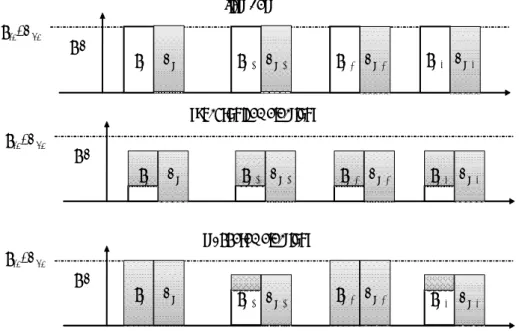
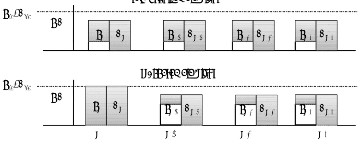
Figure 3 illustrates this result and summarizes the di¤erences between the staggered and the synchronized election regimes. For expositional convenience, we assume in our …gure that the …rst best levels of regional and national public good provision are equal. The …nancing share of the regional government is highlighted in white and the …nancing share of the central government is highlighted in grey.

The lower graph illustrates the result of the staggered regime. On the one hand, the zero …nancing contribution of regional governments in periods where the central government enters illustrates how regional governments exploit their …rst mover advantage. On the other hand, the high contribution share of regional governments in periods when they enter illustrates the power of the central government to enforce a higher overall regional …nancing contribution in the staggered regime.

We can summarize that in every second period (t + 2n; n 2 Z) public con-sumption coincides with the social planner outcome and in every other period (t + 1 + 2n; n_{2 Z) it coincides with the synchronized elections outcome.}

We are now able to make a statement on how the timing of elections a¤ects the softness of budget constraints:

Proposition 2 A decentralized leadership with staggered o¢ ce terms is associated with a higher level of grants than the social planner set-up, but with a lower level of grants than the synchronized elections set-up.

Proof. In the social planner solution we have: (zt+ zt+1)

SP

= (1 + N ) C 2 _G

whereas for the synchronized o¢ ce terms solution we obtain: (zt+ zt+1)

SY

= (1 + N ) C 2 _G g+ G (1 + N ) _G+ _g

!

and for the staggered o¢ ce terms solution grants are given by: (zt+ zt+1)ST = (1 + N ) C 2 G g+ G+ N2 G (1 + N ) _G+ _g ! which implies (zt+ zt+1) SP < (zt+ zt+1) ST < (zt+ zt+1) SY

Staggered elections serve as a discipline device for the regional governments because the central government bene…ts more than the regional governments from its partial leadership position.

5

Welfare Analysis

Due to the results obtained in the previous sections, we are able to unambiguously rank the welfare of the synchronized and staggered o¢ ce term regimes.

Proposition 3 The staggered o¢ ce term regime clearly dominates the synchro-nized o¢ ce term regime and we have the following ranking between outcomes:

R;SP _> R;ST _> R;SY

gSP_t = g_tST > g_tSY gSP_t+1> g_t+1ST = gSY_t+1 GSP_t = GST_t > GSY_t GSP_t+1> GST_t+1= GSY_t+1

Proof. See Appendix 1

We drop in this section the time index for the regional tax rate because the same tax rate is set in in…nite repetition.

The staggered terms of o¢ ce outcome coincides in periods where regional gov-ernments enter o¢ ce with the synchronized o¢ ce terms outcome and in periods where the central government enters with the social planner outcome. Given that the staggered o¢ ce terms regime is e¢ cient half of the time and ine¢ cient half of the time, while the synchronized o¢ ce terms regime is ine¢ cient all of the time, the staggered o¢ ce terms regime clearly dominates.

6

Discussion

6.1

Relaxation of the one-term-of-o¢ ce assumption

One critical assumption of our setup is that governments may stay only for one term of o¢ ce. In this section, we discuss the relaxation of this assumption. Con-sider a game where each government stays in o¢ ce for two terms of o¢ ce, i.e. four periods. Governments enter at date t in the simultaneous regime whereas the regional government enters at date (t + 1) in the staggered regime. Hence, both governments care for periods t to (t + 1) in the synchronized regime, and in the staggered regime the central government considers the utility of the periods t to (t + 3) while the regional government considers (t + 1) to (t + 4), etc. Solving this game by an identical approach as described in the previous sections yields the result illustrated in …gure 4 below, given that governments could commit for all expected o¢ ce periods.

There is no reason for a change of the result in the synchronized regime, because both the regional and the central government have an equal valuation of utility for all periods, and the e¤ect of the interregional externality remains the same. Similarly, in the staggered elections setup, the central government still has an incentive to bind itself for all periods following period t to force future regional governments to …nance, compared to the SY regime, the additional di¤erence of

g+ (1 + N ) G

g+ G

g+(1+N ) G by itself.

However although …gure 4 describes the preferred solution with commitment power over the whole expected o¢ ce duration, there is no reason to assume that this solution can be enforced, given the assumption that governmental programs are set up for one o¢ ce term, but not for longer periods. Knowing that there is scope for renegotiation at each date, where a new government enters or is reelected, makes it not credible that the central government could maintain the preferred allocation at periods (t + 2) and (t + 3) in the staggered regime. Given the lack of credibility, it becomes optimal for the regional government to implement the

g,G g,G g_FB=G_FB synchronized elections staggered elections g_FB=G_FB t+3 t+2 t+1 t g_t+1 G_t+1 g_t+2 G_t+2 g_t+3 G_t+3 g_t G_t g_t+1 G_t+1 g_t G_{t g} t+3 Gt+3 g_t+2 G_t+2

strategic solution st+2 = 0 for date (t + 2). Once the central government enters

o¢ ce at (t + 2) and is able to set-up a new program, it will be irresistible to …nance all public good provision on its own. This in turn renders it optimal for the regional government to exploit its strategic advantage in the same manner as in the setup with the one-o¢ ce term restriction, which yields the initial solution for the staggered o¢ ce term regime.

6.2

The role of the balanced budget constraint

assump-tions

The possibility to freely shift funds from one period to another within one o¢ ce term, along with the assumption of a strict budget balancing constraint over the whole o¢ ce term, seems very strict at …rst glance. Therefore, we discuss in this section the implications of those assumptions, along with the consequences of their relaxation.

First, we turn the attention to the absence of the intra-o¢ ce term budget con-straint. While the absence of this constraint does not imply an uneven distribution of public funds over time in the synchronized regime, it strongly a¤ects the out-come of the staggered o¢ ce terms setup. The result that governments alternate over time between …nancing either a lot or very few of public good provision seems extreme. However, in light of the analysis of political programs, the result has less severe policy implications than it seems at …rst glance. The broad strategic decisions made in the political program like the general tax policy or expenditure choices, e.g. a reform of the social security system, unfold a binding force over the whole term. Unlike in the model where decisions become binding by taking place chronologically before other decisions, real world political programs are unlikely to allot expenditures unevenly over time periods. In this sense, the result of the stag-gered o¢ ce terms regime might be interpreted such that the central government would prefer a larger share of its revenues to be bound in national public programs once it can anticipate the strategic behavior of regional governments. In the same fashion, regional governments might be interested to create a fait accompli with which future central governments have to deal with when setting up their next political programs.

The second potentially controversial part of the budget balancing assumptions is that the budgets need to be balanced at the end of each term of o¢ ce. One possibility to relax this assumption would be to allow the regional and the central governments to borrow. In the model as it stands, this would lead either to an in…nite or to a maximal possible drawing of debt. The reason is that governments do not take into account the utility of public good provision beyond their terms of o¢ ce. Therefore, any sensible relaxation of the balanced budget constraint over

the o¢ ce term should allow governments to take the utility of future payo¤s into account. However, once we allow for the consideration of future payo¤s, there is no incentive to shift debt into the future as long as governments are equally weighting current and future periods. In an intermediate case where future payo¤s are valued by a factor less than one, this would entail indebtedness to some extent. As long as central governments could commit to some optimal level of debt at the beginning of the o¢ ce term, this would not qualitatively a¤ect our results. However, once central governments were able to raise revenues ex-post at the time they decide on the level of grants, this would destroy the regional governments’incentives to raise any revenues and would lead to full central government …nancing of regional public goods.

7

Conclusion

An interesting result of our analysis is that a staggered o¢ ce terms regime always increases welfare. This is due to the fact that central government is able to harden budget constraints at least half of the time by spending most of its funds e¢ ciently in the …rst half of its term of o¢ ce, where “old” regional governments cannot respond strategically. In the second half of the term only a few funds are left over and the central government prefers to spend these funds for national consumption instead of bailing out sub-national jurisdictions. In the synchronized o¢ ce terms regime, this commitment e¤ect is absent and soft budget constraints occur in all of the periods.

Our model implies that central governments devote a smaller share of funds to discretionary grants with staggered elections. This result is of particular impor-tance since discretionary grants are sometimes controversial. One policy implica-tion of our analysis is that central governments should take an active role in setting up the electoral timetable for the …scal discipline of the regional governments as well as the wellbeing of their citizens.

References

Bergvall, D., Charbit, C., Kraan, D-J, & Merk, O. 2006. Intergovernmental Trans-fers and Decentralised Public Spending. OECD Journal of Budgeting, 5, 111– 159.

Besfamille, M., & Lockwood, B. 2008. Bailouts in Federations: Is a Hard Budget Constraint Always Best? International Economic Review, 49(2), 577–593. Breuillé, M-L., Madiès, T., & Taugourdeau, E. 2006. Does Tax Competition Soften

Crivelli, E., & Staal, K. 2008. Size, Spillovers and Soft Budget Constraints. Work-ing Paper Series of the Max Planck Institute for Research on Collective Goods, Max Planck Institute for Research on Collective Goods.

Goodspeed, T. 2002. Bailouts in a Federation. International Tax and Public Finance, 9, 409–421.

Hajnal, Z., & Lewis, P. 2003. Municipal Institutions and Voter Turnout in Local Elections. Urban A¤airs Review, 38(5), 645–668.

Joumard, I., Price, R, & Sutherland, D. 2005. Fiscal Rules for Sub-Central Gov-ernments. OECD Economics Department Working Papers No. 465.

Koethenbuerger, M. 2007. Ex-Post Redistribution in a Federation: Implications for Corrective Policy. Journal of Public Economics, 91(3-4), 481–496.

Kornai, J. 1979. Resource-Constrained versus Demand-Constrained Systems. Econometrica, 47(4), 801–819.

Kornai, J. 1980. Economics of Shortage. Amsterdam: North-Holland publishing company.

Kornai, J., Maskin, E., & Roland, G. 2003. Understanding the Soft Budget Con-straint. Journal of Economic Literature, 41(4), 1095–1136.

Qian, Y., & Roland, G. 1998. Federalism and the Soft Budget Constraint. Amer-ican Economic Review, 88(5), 1143–1162.

Rodden, J., Eskeland, G. S., & Litvack, J. 2003. Fiscal Decentralization and the Challenge of Hard Budget Constraints. MIT Press.

Samuels, D. 2004. Presidentialism and Accountability for the Economy in Com-parative Perspective. American Political Science Review, 98, No. 3, 425–436. Shugart, M. 1995. The Electoral Cycle and Institutional Sources of Divided Pres-idential Government. The American Political Science Review, 89, No. 2, 327–343.

Vigneault, M. 2007. Grants and Soft Budget Constraints. In: Shah, Anwar, & Boadway, Robin (eds), Intergovernmental Fiscal Transfers: Principles and Practice. Washington, DC: The World Bank.

Wildasin, D. 1997. Externalities and Bailouts. Hard and Soft Budget Constraints in Intergovernmental Fiscal Relations. Worldbank Policy Research Working Paper, 1843.

8

Appendix

8.1

Appendix 1 Welfare analysis

The following table gives the results of the government’s tools

SP SY ST gt g g g+ G g+(1+N ) G g gt+1 g g g+ G g+(1+N ) G g g+ G g+(1+N ) G Gt (1 + N ) G (1 + N ) G g+ G g+(1+N ) G (1 + N ) G Gt+1 (1 + N ) G (1 + N ) G g+ G g+(1+N ) G (1 + N ) G g+ G g+(1+N ) G R 2 g+ G(1 + N ) (1 + N ) C g + G (1 + N ) C 2 g+ G(1 + N ) N _G (1 + N ) C From the comparison of the results we obtain:

R;SP _> R;ST _> R;SY

g_tSP = gST_t > gSY_t g_t+1SP > gST_t+1= g_t+1SY GSP_t = GST_t > GSY_t GSP_t+1 > GST_t+1 = GSY_t+1 The utilities are given by

USP = 2w + N C 2 _g+ (1 + N ) _G + 2 _gln _g+ 2 (1 + N ) _Gln _G(1 + N ) and USY = 2w + N C 2 _g+ _G + 2 _g+ (1 + N ) _G ln g + G g+ (1 + N ) G +2 _gln _g+ 2 _G(1 + N ) ln (1 + N ) _G and UST = 2w + N C + 2 _gln _g + 2 (1 + N ) _Gln (1 + N ) _{G g} + _G (1 + N ) _G+ _g + _g + (1 + N ) _G ln g+ G g+ (1 + N ) G

The di¤erence between the ST welfare function and the SY welfare function is given by USY UST = _g+ (1 + N ) _G ln g+ G g + (1 + N ) G + 1 g+ G g+ (1 + N ) G ! < 0 since if we set x = g+ G g+ (1 + N ) G the function f (x) = 1 x + lnx < 0 _{8 x} and USP UST = _g + (1 + N ) _G + _g+ _{G g} + (1 + N ) _G ln g + G g+ (1 + N ) G ! = _g+ (1 + N ) _G 1 + g+ G g+ (1 + N ) G ln g+ G g+ (1 + N ) G ! > 0 then USP > UST > USY