HAL Id: hal-00807355
https://hal.archives-ouvertes.fr/hal-00807355
Submitted on 3 Apr 2013
HAL is a multi-disciplinary open access
archive for the deposit and dissemination of
sci-entific research documents, whether they are
pub-lished or not. The documents may come from
teaching and research institutions in France or
abroad, or from public or private research centers.
L’archive ouverte pluridisciplinaire HAL, est
destinée au dépôt et à la diffusion de documents
scientifiques de niveau recherche, publiés ou non,
émanant des établissements d’enseignement et de
recherche français ou étrangers, des laboratoires
publics ou privés.
Bifurcation of hyperbolic planforms
Pascal Chossat, Grégory Faye, Olivier Faugeras
To cite this version:
Pascal Chossat, Grégory Faye, Olivier Faugeras. Bifurcation of hyperbolic planforms. Journal of
Nonlinear Science, Springer Verlag, 2011, 21 (4), pp.465-498. �10.1007/s00332-010-9089-3�.
�hal-00807355�
Bifurcation of hyperbolic planforms
Pascal Chossat
1,2, Gr´egory Faye
1, and Olivier Faugeras
11NeuroMathComp Laboratory, INRIA, Sophia Antipolis, CNRS, ENS Paris, France
2
Dept. of Mathematics, JAD Laboratory, CNRS and University of Nice Sophia-Antipolis, Parc Valrose, 06108 Nice Cedex 02, France
July 16, 2010
Abstract
Motivated by a model for the perception of textures by the visual cortex in primates, we analyse the bifurca-tion of periodic patterns for nonlinear equabifurca-tions describing the state of a system defined on the space of structure tensors, when these equations are further invariant with respect to the isometries of this space. We show that the problem reduces to a bifurcation problem in the hyperbolic plane D (Poincar´e disc). We make use of the concept of periodic lattice in D to further reduce the problem to one on a compact Riemann surface D/Γ, where Γ is a cocompact, torsion-free Fuchsian group. The knowledge of the symmetry group of this surface allows to carry out the machinery of equivariant bifurcation theory. Solutions which generically bifurcate are called ”H-planforms”, by analogy with the ”planforms” introduced for pattern formation in Euclidean space. This concept is applied to the case of an octagonal periodic pattern, where we are able to classify all possible H-planforms satisfying the hypotheses of the Equivariant Branching Lemma. These patterns are however not straightforward to compute, even numerically, and in the last section we describe a method for computation illustrated with a selection of images of octagonal H-planforms.
Keywords: Equivariant bifurcation analysis; neural fields; Poincar´e disc; periodic lattices; hyperbolic planforms; irreductible representations; Laplace-Beltrami operator.
1
Introduction
In a recent paper [11] a model for the visual perception of textures by the cortex was proposed, which assumes that populations of neurons in each so-called ”hypercolumn” of the visual cortex layer V1 are sensitive to informations carried by the structure tensor of the image (in fact, of a small part of it since each hypercolumn is dedicated to a specific part of the visual field). The structure tensor is a2× 2 positive definite, symmetric matrix, the eigenvalues of which characterize to some extent the image geometric properties like the presence and position of an edge, the contrast, etc. This led to write the average membrane potentialV of the populations of neurons in a hypercolumn as a function of the structure tensor (and time). The equations that govern the evolution of the average membrane potential are ∂V ∂τ(T , τ) = −αV (T , τ) + � H w(T , T�)S(V (T�, τ )) dT�+ I(T , τ) (1) whereT , T� ∈ SDP (2) (the space of structure tensors), S is a smooth function R → R of sigmoid type (S(x) → ±1 as x → ±∞), I corresponds to some input signal coming from different brain areas such as the thalamus andw(T , T�) is a function which expresses the interaction between the populations of neurons of types
T and T�in the hypercolumn. We can introduce a distance on the set of structure tensors by noting that it has the
structure of a homogeneous space for the group of invertible matricesGL(2, R) acting by coordinate change on quadratic forms associated with the structure tensors [40]: for anyT ∈ SDP (2) and G ∈ GL(2, R), we define G· T = tG
T G. This induces a Riemannian metric on the tangent space: gT(A, B) = tr(T−1AT−1B) and the
corresponding distance inSDP (2) is given by (see [32])
d0(T1,T2) = � log2λ1+ log2λ2 (2)
a
rX
iv:
1007.2492v1 [m
a
th.D
S
] 15 J
ul
2010
whereλ1, λ2 are the eigenvalues ofT1−1T2. Because of its invariance this distance is biologically plausible
since the neurons have no obvious way of knowing in which coordinate system are expressed the components of the structure tensors and this leads to the assumption that the functionw is insensitive to coordinate changes in SDP (2). This implies that w is in fact a function of the distance d0:
w(T , T�) = f (d
0(T , T�)) (3)
As a consequence, the equation (1) is invariant under the action of the isometry groupGL(2, R).
Assume now that there is no input: I = 0, and that V = 0 is a solution of (1) (we can assume w.l.o.g. that S(0) = 0). If the slope µ = S�(0) is small enough, small perturbations of this basic state are damped to 0 and the
basic state is stable. We can however expect that ifµ exceeds a critical value an instability will grow and lead to a new state which need not be invariant under the action ofGL(2, R). In other word we expect pattern formation through spontaneous symmetry breaking, a phenomenon which has been widely studied in other contexts in the last 40 years (see [25] for a review). From the mathematical point of view the theoretical framework is the well-established bifurcation theory with symmetry [21], [12]. There is however a basic difference between the problem at hand and previous studies in pattern formation and symmetry-breaking bifurcation: the symmetries (isometries) are not Euclidean. Moreover the groupGL(2, R) being non compact, the spectrum of the equivariant linear operators is continuous and eigenvalues have infinite multiplicity in general. This is also true when the symmetry group is the group of displacements and reflections in Euclidean space. In this case a rational approach is to resctrict the analysis to the bifurcation of patterns which are periodic (in space) with a period equal to2π/k wherek is the wave number of the most unstable Fourier modes. This hypothesis is supported by observations (to some extent) and it provides a framework which is suitable for the bifurcation analysis. Namely, the spectrum of operators restricted to functions which are invariant on a periodic lattice is discrete and consists of eigenvalues with finite multiplicity. This allows to fully exploit the power of equivariant bifurcation theory and to describe the different types of bifurcated solutions by their (remaining) symmetries.
We would like to proceed in a similar way for equation (1), that is to consider solutions which are periodic in the space of structure tensors (one has to give a precise meaning to this statement) and then apply equivariant bifurcation methods to describe the set of solutions. We are not addressing here the question of the relevance of looking for such solutions, neither from the neurophysiological point of view, nor even from the point of view of their stability under perturbations which do not have the same periodicity (or no periodicity at all). Let us mention the fact that in [11] we identified families of subgroups of the group of isometries of the set of structure tensors that naturally arose from the analysis of the retinal input to the hypercolumns in visual area V1. These subgroups, which we called neuronal Fuchsian groups, have the property that the membrane potential functions are invariant under their action. This is one example of the neurophysiological relevance of looking for solutions of (1) that are periodic in this sense but it certainly does not give the final answer: These difficult questions will be addressed subsequently. Let us point out that, on the other hand, a classification of possible periodic patterns should be largely independent of the model equations as long as these equations share some basic properties (likeGL(2, R) invariance). In this paper we shall therefore not focus on equation (1) and our results would apply equally to other models such as reaction-diffusion or Swift-Hohenberg equations with Laplace-Beltrami operator inSDP (2)).
The structure of the paper is as follows:
1. In section2 we introduce the necessary basic material from hyperbolic geometry. Periodic lattices and functions are defined inSDP (2) and it will be shown that the problem can be decoupled and reduced to looking for periodic patterns in the hyperbolic plane (we shall work with its Poincar´e disc representation D).
2. In section3we set the bifurcation problem for periodic patterns in D. Applying the equivariant branch-ing lemma [21] (or isolated stratum principle in the variational case), this leads us to defining hyperbolic
planforms, which are the hyperbolic counterparts of the planforms defined in the Euclidean case (see [17]). 3. In section4the methods of section3are applied to the case of a regular octagonal pattern for which we can
describe all planforms which result from the applicaiton of the equivariant branching lemma.
4. In section5we compute eigenvalues and eigenfunctions of the Laplace-Beltrami operator in the hyperbolic octagon in order to exhibit hyperbolic planforms which satisfy certain isotropy conditions.
2
Periodic lattices and functions in the space of structure tensors
2.1
The space SDP(2)
The following decomposition will prove to be very convenient. Letξ2be the determinant of
T ∈ SDP (2). We setξ > 0 by convention. WritingT = ξT�, we see thatSDP (2) = R+
∗ × SSDP (2) where SSDP (2) denotes
the subspace of tensors with determinant 1. In the open coneSDP (2) the surface SSDP (2) is a hyperboloid sheet and it can be shown that it carries a metric induced by the metricg which is just the usual metric of the hyperbolic plane. The isometry group of displacements inSSDP (2) is the special linear group SL(2, R), and indeed we may also write the group of orientation preserving isometriesGL+(2, R) = SL(2, R)× R+
∗ acting on
a tensorT = (T�, ξ) by
(Γ, α)· (T�, ξ) = (tΓ
T�Γ, α2ξ).
(4) We now identifySDP (2) with the ”half” open cylinderD × R+
∗, whereD is the Poincar´e disc, through the
following change of variables. LetT =
�
x1 x3
x3 x2
�
withx1> 0 and x1x2− x23> 0. We set
xi = z3x˜i, i = 1, 2, 3, z3> 0, ˜x1x˜2− ˜x23= 1.
Now the hyperbolic planeSSDP (2) is further identified withD through the change of coordinates ˜ x1 = (1+z1) 2+z2 2 1−z2 1−z22 ˜ x2 = (1−z1) 2 +z2 2 1−z2 1−z 2 2 ˜ x3 = 1−z2z22 1−z 2 2 (5)
These formulas define a diffeomorphism
Θ : (x1, x2, x3)∈ SDP (2) �→ (z1, z2, z3)∈ D × R+∗ (6)
The group of direct isometries (displacements) inD × R+∗ isSU (1, 1)× R+∗ whereSU (1, 1) =
� α β ¯ β α¯ � with |α|2
− |β|2= 1. Including orientation reversing isometries would replace SU (1, 1) by U (1, 1).
Proposition 1. The metric carried toD × R+∗ byΘ is (up to a normalization coefficient)
g1(z1, z2, z3) = 4(dz2 1+ dz22) (1− z2 1− z22)2 +dz 2 3 z2 3 (7)
Proof. The fact that the decomposition is diagonal follows directly from the direct product decomposition and group action (4). In order to compute the precise expression for the metric, let us first express the formg in SDP (2) in suitable coordinates of the tangent space (which is the space of symmetric 2× 2 matrices). Such a basis is given, at any tensorT , by
∂ ∂x1 = � 1 0 0 0 � ∂ ∂x2 = � 0 0 0 1 � ∂ ∂x3 = � 0 1 1 0 �
Then a straightforward calculation shows that
g(x1, x2, x3) = z3−4[x22dx12+ 2x23dx1dx2− 4x2x3dx1dx3
+x2
1dx22− 4x1x3dx2dx3+ 2(x1x2+ x23)dx23].
The proposition follows by applying the pull-backΘ∗to this form.
Corollary 1. The volume element in thezjcoordinates is
dV = 4 dz1dz2dz3 (1− z2
1− z22)2z3
Corollary 2. The Laplace -Beltrami operator inD × R+∗ inzjcoordinates is � = (1− z 2 1− z22)2 4 � ∂2 ∂z2 1 + ∂ 2 ∂z2 2 � + z3 ∂ ∂z3 + z2 3 ∂2 ∂z2 3 (9)
We note�Dthe first term on the r.h.s.
Let us now compute the distanced inD × R+
∗. We set z= (z1, z2, z3) and z�= (z1�, z2�, z3�). Then
Proposition 2. d(z, z�) = � (d2((z1, z2), (z1�, z2�))2+ log 2(z3 z� 3 ) (10)
whered2denotes the distance in the Poincar´e disc.
Proof. We start from expression (2) which gives the distance between two tensorsT1 andT2. LetT = z3T ,˜
T�= z�
3T˜�andα = z3/z3�. We noteλ, 1/λ the eigenvalues of ˜T−1T˜�. Then
d0(T , T�)2= log2αλ + log2
α
λ = 2 log
2α + 2 log2λ = 2 log2α + d
0( ˜T , ˜T�)2.
Butd0( ˜T , ˜T�) = d2((z1, z2), (z1�, z�2)), hence the result.
Note that the distance inD is given by the following formula where z, z�are complex numbers in the unit disc.
d2(z, z�) = 2 arctanh|z − z � | |1 − zz�|, (11)
2.2
Periodic lattices in
D × R
+ ∗Let us recall first some basic properties of the group of isometries in the hyperbolic plane (which we shall always identify with the Poincar´e discD in the sequel). We refer to textbooks in hyperbolic geometry for details and proofs. The direct isometries (preserving the orientation) inD are the elements of the special unitary group, noted SU(1, 1), of 2× 2 Hermitian matrices with determinant equal to 1. Given
γ = � α β β α � such that|α|2− |β|2= 1, the corresponding isometryγ is defined by
γ· z = αz + β
βz + α, z∈ D (12)
Orientation reversing isometries ofD are obtained by composing any transformation (12) with the reflection κ : z�→ z. The full symmetry group of the Poincar´e disc is therefore
U(1, 1) = SU(1, 1)∪ κ · SU(1, 1).
These isometries preserve angles, however they do not transform straight lines into straight lines. Given two pointsz �= z�in
D, there is a unique geodesic passing through them: the portion in D of the circle containing z andz�and intersecting the unit circle at right angles. This circle degenerates to a straight line when the two points
lie on the same diameter. Any geodesic uniquely defines the reflection through it. Reflections are orientation reversing, one representative being the complex conjugation:κ· z = z.
We distinguish three different kinds of direct isometries in D, according to which conjugacy class of the following one parameter subgroups it does belong:
Definition 1. K = {rϕ= � eiϕ/2 0 0 e−iϕ/2 � , ϕ∈ S1 } A = {at= � cosh t/2 sinh t/2 sinh t/2 cosh t/2 � , t∈ R} N = {ns= � 1 + is −is is 1− is � , s∈ R}
Note thatrϕ·z = eiϕz for z∈ D and also, at·0 = tanh(t). The elements of A are sometimes called “boosts”
[4]. The following theorem is called the Iwasawa decomposition (see [27]). Theorem 1.
SU(1, 1) = K· A · N
The orbits ofA converge to the same limit points b±1 =±1 on the unit circle when t → ±∞. In particular the
diameter(b−1, b1) is the orbit{x = tanh(t), t ∈ R}. The orbits of N are the circles tangent to the unit circle at
b1. These circles are called horocycles with limit pointb1(N is called the horocyclic group). The orbits of K are
circles insideD (they coincide with Euclidean circles only when they are centered at the origin).
Isometries of the typesK, A, N are respectively called elliptic, hyperbolic and parabolic. Elliptic isometries have one fixed point inD while hyperbolic isometries have two fixed points on the boundary ∂D and parabolic isome-tries have one fixed point on∂D (hence ”at infinity”). Hyperbolic isometries play the same role as translations in Euclidean space while parabolic isometries have no counterpart. There is however one important difference with Euclidean translations: two hyperbolic translations do not commute in general. The fundamental difference from this point of view betweenD and the Euclidean plane R2 is that the latter is itself an Abelian group while
D � SU(1, 1)/SO(2, R) is not a group. This makes its analysis, especially its Fourier analysis, harder and less intuitive.
We can now define a (periodic) lattice inD and in D × R∗. LetΓ be a discrete subgroup of SU (1, 1) such that
the orbits of points inD under the action of Γ have no accumulation point in D. This is a Fuchsian group. To any Fuchsian group we can associate a fundamental domain which is the closure, notedFΓ, of an open set
o
FΓ ⊂ D
with the following properties [28]: (i) ifγ�= Id ∈ Γ, then γFΓ∩ o FΓ =∅; (ii) � γ∈Γ γFΓ =D.
HenceFΓgenerates a periodic tiling (or tessellation) ofD. A fundamental domain need not be a compact subset
ofD (it may have vertices on the circle at infinity ∂D). When it does, Γ is called a cocompact Fuchsian group. In this caseΓ contains no parabolic element, its area is finite and a fundamental domain can always be built as a polygon (the Dirichlet region, see [28]). As mentioned in the introduction we identified in [11] a family of Fuchsian groups, some of them compact, that naturally arose from the analysis of the symmetries in the spatial distribution of the photoreceptors in the retina.
The following definition is just a translation to the hyperbolic plane of the definition of an Euclidean lattice. Definition 2. A lattice group ofD is a cocompact Fuchsian group which contains no elliptic element.
The action of a lattice group has no fixed point, therefore the quotient surfaceD/Γ is a (compact) manifold and it is in fact a Riemann surface. A remarkable theorem states that any compact Riemann surface is isomorphic to a lattice fundamental domain ofD if and only if it has genus g ≥ 2 [28]. The caseg = 1 corresponds to lattices in the Euclidean plane (in this case there are three kinds of fundamental domains: rectangles, squares and hexagons). The simplest lattice inD, with genus 2, is generated by an octagon and will be studied in detail in Section4.
Given a lattice, we may ask what is the symmetry group of the fundamental domain FΓ, identified with
the quotient surfaceD/Γ. Indeed, this information will play a fundamental role in the subsequent bifurcation analysis. In the case of Euclidean lattice, the quotient R2/Γ is a torusT (genus one surface), and the group of automorphisms isH � T where H is the holohedry of the lattice: H = D2, D4orD6for the rectangle, square
and hexagonal lattices respectively. In the hyperbolic case the group of automorphisms of the surface is finite. In order to build this group we need first to introduce some additional definitions.
Tilings of the hyperbolic plane can be generated by reflections through the edges of a triangleτ with vertices P , Q, R and angles π/�, π/m and π/n respectively, where �, m, n are integers such that 1/� + 1/m + 1/n < 1 [28].
Remember that reflections are orientation-reversing isometries. We noteκ, κ�andκ��the reflections thro ugh
the edgesP Q, QR and RP respectively (Figure1). The group generated by these reflections contains an index 2 Fuchsian subgroupΛ called a triangle group, which always contains elliptic elements because the product of the reflections through two adjacent edges of a polygon is elliptic with fixed point at the corresponding vertex. One easily shows thatΛ is generated by the rotations of angles 2π/l, 2π/m and 2π/n around the vertices P , Q,
!
"
π/
#
π/
$
π/
%
κ
κ
&
κ
'
Figure 1: The triangleτ , also noted T (2, 3, 8). The values of l, m, and n are l = 8, m = 2 and n = 3.
−1 −0.5 0 0.5 1 −1 −0.8 −0.6 −0.4 −0.2 0 0.2 0.4 0.6 0.8 1 x axis y axis
Figure 2: Tesselation of the hyperbolic octagon with the triangleT (2, 3, 8), colored in purple in the plot. We define two points �S and �S. �S is the center of the rotation ˆσ by π (modΓ), see text in subsection4.1. �S is the center of the rotation˜σ by π (modΓ), see text in subsection4.1.
R re spectively. A fundamental domain of Λ is the ”quadrangle” FΛ = τ ∪ κτ [28]. Note thatFΛ � D/Λ is
a sphere (genus 0 surface) obtained by identifying the three edges ofτ . The subgroup of hyperbolic translations inΛ is a lattice group Γ, normal in Λ, whose fundamental domain is filled with copies of the basic tile τ . The group of orientation-preserving automorphisms ofFΓ � D/Γ is therefore G = Λ/Γ. From the algebraic point of
view,G is generated by three elements a, b, c satisfy therelations a� = bm= cn = 1 and a
· b · c = 1. We say thatG is an (l, m, n) group. Taking account of orientation-reversing isometries, the full symmetry group of FΓis
G∗= G
∪ κG = G � Z2(κ). This is also a tiling group of FΓwith tileτ : the orbit G∗τ fills FΓand its elements
can only intersect at their edges.
Given a lattice, how to determine the groupsG and G∗? The following theorem gives conditions for this, see
[9].
Theorem 2. An(l, m, n) group G is the tiling rotation group of a compact Riemann surface of genus g if and only
if its order satisfies the Riemann-Hurwitz relation
|G| = 1 2g− 2 − (1 �+ 1 m+ 1 n) .
Tables of triangle groups for surfaces of genus up to 13 can be found in [9]. These definitions extend naturally toSDP (2)� D × R∗as follows.
Definition 3. A lattice group ofD × R∗is a subgroup of the formΓ× Ξ where Γ is a lattice group acting in D
andΞ is a non trivial discrete subgroup of R∗.
Any discrete subgroup of R∗is generated by a positive numbera and can be further identified with Z: Ξ = {an, n
∈ Z}. A fundamental domain for Γ × Ξ is a ”box” FΓ× [1, a].
2.3
Plane waves in SDP(2)
Let us first recall the Euclidean setting for functions defined in R3(we could take any other Rn,n > 0). In this case every function of the formeλk·rwhere k∈ R3is a unit vector, is an eigenfunction of the Laplace operator in
R3:
∆eλk·r=−λ2eλk·r, r∈ R3.
The fact that the eigenvalues do not depend upon the direction of the wave vector k reflects the rotational invariance of the Laplace operator. Moreover if we takeλ = iα, α∈ R, then eλk·r is invariant under translations in R2by
any vector e satisfying the condition k· e = 2nπ where n ∈ Z (it clearly does not depend upon the coordinate along the axis orthogonal to k). The functionseiαk·rare elementary spatial waves in R3.
Now, givenα > 0 and a basis of unit vectors{k1, k2, k3} of R3we can define the translation groupL spanned
by ei,i = 1, 2, 3, such that ki· ej = 2π/αδij. HenceL is a lattice group of R3. It defines a periodic tiling,
the fundamental domain of which is a compact cell which we may identify with the quotient space R3/L and which we can identify with a 3-torus. Any smooth enough function in R3 which is invariant under the action of L can be expanded in a Fourier series of elementary spatial waves eiα(mk1+nk2+pk3)·r, m, n, p ∈ Z. The
Laplace operator in the space of square-integrable functions in R3/L is self-adjoint and its spectrum consists of real isolated eigenvalues with finite multiplicities. The multiplicity depends upon the holohedry of the lattice, which we defined in the previous section (the largest subgroup ofO(3) leaving invariant the lattice). There are finitely many holohedries (see [31] for details). It follows from the above considerations that by restricting the analysis to classes of functions which are invariant under the action of a lattice group, one can apply standard techniques of equivariant bifurcation theory to assert the generic existence of branches of solutions of Euclidean invariant bifurcation problems, which are spatially periodic with respect to lattice groups and whose properties are largely determined by the holohedry of the lattice [21],[17]. Note also this was the approach of [7] for the analysis of the occurence of visual hallucinations in the cortex.
We wish to apply the same idea to bifurcation problems defined in SDP (2). For this we need to define elementary eigenfunctions of the Laplace-Beltrami operator such that spatially periodic functions (in a sense to be defined later) can be expanded in series of these elementary ”waves” inSDP (2). In the sequel� will denote the Laplace-Beltrami operator inSDP (2) or, equivalently, inD × R+
∗.
Letb be a point on the circle ∂D, which we may take equal to b1 = 1 after a suitable rotation. For z ∈ D,
we define the ”inner product”�z, b� as the algebraic distance to the origin of the (unique) horocycle based at b and passing throughz. This distance is defined as the hyperbolic signed length of the segment Oξ where ξ is the
intersection point of the horocycle and the line (geodesic)Ob. Note that�z, b� does not depend on the position of z on the horocycle. In other words,�z, b� is invariant under the action of the one-parameter group N (see definition above). The ”hyperbolic plane waves”
eρ,b(z) = e(iρ+ 1 2)�z,b�, ρ∈ C, satisfy −�Deρ,b= (ρ2+ 1 4)eρ,b.
where�Dis defined in Corollary2. These are the elementary eigenfunctions with which Helgason built a Fourier
transform theory for the Poincar´e disc, see [24]. It follows from Helgason’s theory that any eigenfunction of�D
can be expressed as an integral over the boundary elements:
Theorem 3. [24] Any eigenfunction of the operator−�Dadmits a decomposition of the form
�
∂D
eρ,b(z)dTρ(b)
whereTρis a distribution defined on the circle∂D and the eigenvalue is ρ2+14.
Real eigenvalues−(ρ2+1
4) of�Dcorrespond to taking ρ real or ρ∈ iR. The latter case is irrelevant for our
study as it corresponds to exponentially diverging eigenfunctions. Therefore the real spectrum of� is continuous and is bounded from above by−1/4. By using (9) we extend Theorem3toD × R+∗:
Corollary 3. (i) Let us note z= (z1, z2, z3)∈ D × R+∗ andz = z1+ iz2. The function
ψρ,b,β(z) = eρ,b(z) ei log β log z3 (13)
satisfies the relation�ψρ,b,β=−(ρ2+14+ log2β)ψρ,b,β.
(ii) Any eigenfunction of� admits a decomposition of the form
ei log β log z3
�
∂D
eρ,b(z) dTρ(b). (14)
From there we can extend the definition (and properties) of the Fourier transform in the hyperbolic plane given by Helgason [24] to the spaceD × R+∗:
Definition 4. Given a functionf onD × R+
∗, its Fourier transform is defined by
˜
f (ρ, b, β) = �
D×R+
∗
f (z)e−ρ,b(z)e−i log β log z3dz (15)
In the following we will look for solutions of bifurcation problems inD × R+∗, which are invariant under the
action of a lattice group: (γ, ξ)· u(z, z3) = u(γ−1z, ξ−1z3) = u(z, z3) for γ ∈ Γ, ξ ∈ Ξ. This boils down to
looking for the problem restricted to a fundamental domain with suitable boundary conditions imposed by the Γ-periodicity, or, equivalently, to looking for the solutions of the problem projected onto the orbit spaceD/Γ×R+
∗/Ξ
(which inherits a Riemannian structure fromD × R+
∗). Because the fundamental domain is compact, it follows
from general spectral theory that−� is self-adjoint, non negative and has compact resolvent in L2(D/Γ×R+
∗/Ξ)
[10]. Hence its spectrum consists of real positive and isolated eigenvalues of finite multiplicity.
Coming back to Theorem3, we observe that those eigenvalues λ of−�D which correspond toΓ-invariant
eigenfunctions, must have ρ ∈ R or ρ ∈ iR. The case ρ real corresponds to the Euclidean situation of planar waves with a given wave number, the role of which is played by ρ inD. In this case the eigenvalues of −�D
satisfy1/4 < λ. On the other hand there is no Euclidean equivalent of the case ρ∈ iR, for which the eigenvalues 0 < λ ≤ 1/4 are in finite number. It turns out that such ”exceptional” eigenvalues do not occur for ”simple” groups such as the octagonal group to be considered in more details in the Section4. This follows from formulas which give lower bounds for these eigenvalues. Let us give two examples of such estimates (derived by Buser [10], see also [27]): (i) ifg is the genus of the surfaceD/Γ, there are at most 3g − 2 exceptional eigenvalues; (ii) ifd is the diameter of the fundamental domain, then the smallest (non zero) eigenvalue is bounded from below by �
Suppose now that the eigenfunction in Theorem3isΓ-periodic. Then the distribution Tρsatisfies the following
equivariance relation [33]. Letγ(θ) denote the image of θ∈ ∂D under the action of γ ∈ Γ. Then Tρ(γ· θ) = |γ�(θ)|
1 2+iρT
ρ(θ).
As observed by [36], this condition is not compatible withTρbeing a ”nice” function. In fact, not only does there
not exist any explicit formula for these eigenfunctions, but their approximate computation is itself an uneasy task. We shall come back to this point in subsequent sections.
3
Bifurcation of patterns in SDP(2)
We now consider again equation (1), which we set inD × R+
∗ by the change of coordinates (6). AssumingI = 0
(no external input) and the invariance hypothesis (3) for the connectivity functionw, and after a choice of time scale such thatα = 1, the equation reads
∂V
∂τ =−V + µw ∗ V + R(V ) (16) where:
• µ = S�(0),
• w ∗ V denotes the convolution product�D×R+ ∗ w(z, z
�)V (z�) dz�(withw(z, z�) = f (d(z, z�))),
• R(V ) stands for the remainder terms in the integral part of (3). This impliesR�(0) = 0.
It is further assumed thatf is a ”Mexican hat” function, typically of the form
f (x) = �1 2πσ2 1 e− x2 2σ2 1 − θ�1 2πσ2 2 e− x2 2σ2 2, where σ1< σ2and θ≤ 1.
Let us look at the linear stability of the trivial solution of (16) against perturbations in the form of hyperbolic waves (13) with ρ∈ R. This comes back to looking for σ’s such that
σ=−1 + µ ˆw
wherew is the hyperbolic Fourier transform of w as defined in Definitionˆ 15. The numerical calculation shows that for each value of ρ and β, there exists a valueµ(ρ, β) such that if µ < µ(ρ, β) then all σ’s are negative, while σ = 0 at µ = µ(ρ, β). The ”neutral stability surface” defined by µ(ρ, β) is typically convex and reaches a minimum µc at some values ρc, βc. Therefore when µ < µc the trivial stateV = 0 is stable against such
perturbations while it becomes marginally stable when µ = µc with critical modes ψρc,b,βc, for anyb ∈ S
1
(rotational invariance). Therefore a bifurcation takes place at this critical value.
The situation is absolutely similar if instead of equation 16we consider systems of PDEs inD × R+∗ with
pattern selection behavior and with U (1, 1)× R+
∗ invariance. A paradigm for such systems is the
”Laplace-Beltrami” version of Swift-Hohenberg equation ∂u ∂t = µu− (� + α) 2u + u2, α ∈ R+ ∗. with� as in (9).
It is unconceivable to solve the bifurcation problem at this level of generality, because the fact that the spectrum is continuous plus that each eigenvalue σ has an infinite multiplicity (indifference tob) makes impossible the use of the classical tools of bifurcation theory. As in the Euclidean case of pattern formation, we therefore want to look for solutions in the restricted class of patterns which are spatially periodic. In the present framework, this means looking for bifurcating patterns which are invariant under the action of a lattice groupΓ× Z+
∗ inSU (1, 1)× R+∗.
There is however an immediate big difference with the Euclidean case. While in the latter any critical wave number αc can be associated with a periodic lattice (of period2π/αc), in the hyperbolic case not every value of
to possess eigenfunctions, as defined in Theorem3, which are invariant under a lattice group. We can therefore look for the bifurcation of spatially periodic solutions associated with a given lattice, but these patterns will not in general correspond to the most unstable perturbations unless the parameters in the equations are tuned so that it happens this way. The question of the observability of such patterns is therefore completely open.
We henceforth look for patterns inD × R+∗ which are invariant under a latticeΓ inD and which are periodic, with period2π/βc, in R+∗. This boils down to looking for solutions in the spaceL2(D/Γ × R+∗/βcZ+∗). Note that
R+∗/βcZ+∗ � S1. With a suitable inner product this space admits an orthonormal Hilbert basis which is made of functions of the form
Ψ(z)eni log(βc) log(z3), z
∈ D, n ∈ N whereΨ are the eigenfunctions of� in L2(
D/Γ). As we mentionned in the previous section, these eigenfunctions are not known explicitely. By restricting the ”neutral stability surface”µ(ρ, β) to those values which correspond to eigenfunctions withΓ× βcZ+∗ periodicity, we obtain a discrete set of points on this surface with one minimum
µ0associated with a value ρ0of ρ and β0of β. In general this minimum is unique. Moreover the multiplicity of
the 0 eigenvalue is now finite and this eigenvalue is semi-simple. Let us callX the eigenspace associated with the 0 eigenvalue (thereforeX is the kernel of the critical linear operator).
The full symmetry group ofD/Γ × S1is equal toG∗× O(2) where G∗is the (finite) group of automorphisms
inU (1, 1) of the Riemann surfaceD/Γ (notation of Section2.2) andO(2) is the symmetry group of the circle (generated byS1and by reflection across a diameter). The equation restricted to this class ofΓ
× βcZ+∗-periodic
patterns is invariant under the action ofG∗
× O(2). We can therefore apply an equivariant Lyapunov-Schmidt reduction to this bifurcation problem [12], leading to a bifurcation equation inX
f (x, µ) = 0, x∈ X (17)
wheref : X× R → X is smooth, f(0, 0) = 0, ∂xf (0, 0) is not invertible and f (·, µ) commutes with the action
ofG∗
× O(2) in X.
Now the methods of equivariant bifurcation theory can be applied to (17). In particular we can apply the Equivariant Branching lemma (see [21] for a detailed exposition):
Theorem 4. Suppose the action ofG∗
× O(2) is absolutely irreducible in X (i.e. real equivariant linear maps
inX are scalar multiple of the identity). Let H be an isotropy subgroup of G∗
× O(2) such that the subspace XH=
{x ∈ X | H · x = x} is one dimensional. Then generically a branch of solutions of (17) bifurcates inXH.
The conjugacy class ofH (or isotropy type) is called ”symmetry breaking”.
Let us briefly recall the meaning of this theorem. By equivariance off , any subspace of X defined as XH,H a
(closed) subgroup ofG∗
× O(2), is invariant under f. By the irreducibility assumption, if H = G∗
× O(2), then {x ∈ X | H · x = x} = {0}. Therefore f(0, µ) = 0 for all µ. Now the assumption of absolute irreducibility implies that ∂xf (0, µ) = a(µ)IdXwherea is a smooth real function such that a(0) = 0 and generically a�(0)�= 0.
It follows that if nowH is a subgroup such that dim XH= 1, then equation (17) restricted to this subspace reduces
to a scalar equation0 = a�(0)µx + xh(x, µ) (with h(0, 0) = 0), which has a branch of non trivial solutions by the
implicit function theorem.
Remark 1:the word ”generically” can be interpreted as follows: the result will fail only if additional degeneracies are introduced in the equations. See [12] and [21] for a rigorous definition and proof.
Remark 2:the assumption of absolute irreducibility is itself generic (in the above stated sense) for one-parameter steady-state bifurcation problems. A given irreducible representation of a compact or finite group need not be absolutely irreducible, this fact has to be proven.
Remark 3:Theorem4does not necessarily give an account of all possible branches of solutions of (17), see [12]. It gives nevertheless a large set of generic ones. To go further it is necessary to compute the equivariant structure off , or at least of its Taylor expansion to a sufficient order. The same is true if one wants to determine the stability of the bifurcated solutions, within the class ofΓ× S1periodic solutions of the initial evolution equation.
This theorem, together with the knowledge of the lattices and the (absolutely) irreducible representations of the groupsG∗, gives us a mean to classify the periodic patterns which can occur in
D × R+
∗. By analogy with
the Euclidean case (bifurcation of spatially periodic solutions in the Euclidean space), we call H-planforms the solutions of aU (1, 1) (resp. GL(2R)) invariant bifurcation problem inD (resp. D × R+
∗), which are invariant by
a lattice groupΓ (resp. Γ× S1).
Being interested here in the classification of solutions rather than in their actual computation for a specific equation, all remains to do is to determine the absolutely real irreducible representations of the groupG∗
× O(2) and the computation of the dimensions of the subspacesXH). For this purpose we can get rid of the S1component
of the domain of periodicity. Indeed letH = H1× H2 be an isotropy subgroup for the representation R of
G∗× O(2) acting in X. Then X = V ⊗ W and R = S ⊗ T , where S is an irreducible representation G∗inV
andT is an irreducible representation of O(2) in W [37], and thereforeH1acts inV and H2acts inW . Now we
have the following lemma, the proof of which is straightforward: Lemma 1. dim(XH) = 1 if and only if dim(VH1) = dim(WH2) = 1.
Now, the irreducible real representations ofO(2) are well-known: they are either one dimensional (in which case every point is rotationally invariant) or two-dimensional, and in the latter case the only possible one dimen-sional subspacesWH2 are the reflection symmetry axes in R2(which are all equivalent under rotations inO(2)).
It follows that the classification is essentially obtained from the classification of the isotropy subgroupsH1of the
irreducible representations ofG∗.
Once the irreducible representations are known, this can be achieved by applying the ”trace formula” [21,12]: Proposition 3. LetH be a subgroup of G∗acting in a spaceV by a representation ρ : G∗
→ Aut(V ), then dim(VH) = 1 |H| � h∈H tr(ρ(h)) (18)
Note thattr(ρ) is the character of the representation ρ (a homomorphism G∗
→ C). What is really needed to apply the Equivaraint Branching Lemma is therefore the character table of the representations. In the next section we investigate this classification in the case when the lattice is the regular octogonal group.
4
A case study: the octagonal lattice
According to the comment following Lemma1, in all of this section we only consider the classification of isotropy subgroups satisfying the conditions of the equivaraint branching lemma in the Poincar´e discD.
4.1
The octagonal lattice and its symmetries
Among all lattices in the hyperbolic plane, the octagonal lattice is the simplest one. As before we use the Poincar´e disc representation of the hyperbolic plane. Then the octagonal lattice groupΓ is generated by the following four hyperbolic translations (boosts), see [4]:
g0= � 1 +√2 �2 + 2√2 � 2 + 2√2 1 +√2 � (19)
andgj = rjπ/4g0r−jπ/4,j = 1, 2, 3, where rϕ indicates the rotation of angle ϕ around the origin inD. The
fundamental domain of the lattice is a regular octagonO as shown in Figure. The opposite sides of the octagon are identified by periodicity, so that the corresponding quotient surfaceD/Γ is isomorphic to a ”double dough-nut” (genus two surface) [4]. Note that the same octagon is also the fundamental domain of another group, not isomorphic toΓ, obtained by identifying not the opposite sides but pairs of sides as indicated in Figure. This is called the Gutzwiller octagon. A procedure of classification of the lattices using graphs is presented in [34]. For us however there is no difference between the two kinds of octagons because we are really interested in the full symmetry group of the pattern generated byΓ, which includes the rotations rjπ/4,j = 1,· · · , 8, and therefore
the boostsrπ/2g0−1,g1r−π/2and their conjugates by the rotationrπ, which are precisely the generators of the
Gutzwiller lattice group.
We now determine what is the full symmetry groupG∗of the octagonal lattice, or equivalently, of the surface
D/Γ. Clearly the symmetry group of the octagon itself is part of it. This is the dihedral group D8generated by the
rotationrπ/4and by the reflection κ through the real axis, but there is more. We have seen in Section2.2that the
groupG∗= Λ/Γ, Λ being the triangle group generated by reflections through the edges of a triangle τ which tiles
(by the action ofΛ/Γ) the surfaceD/Γ. The smallest triangle (up to symmetry) with these properties is the one shown in Figure1. It has angles π/8, π/2 and π/3 at vertices P = O (the center ofD), Q, R respectively, and its area is, by Gauss-Bonnet formula, equal to π/24. There are exactly 96 copies of τ filling the octagon, hence |G∗
| = 96. The index two subgroup G of orientation-preserving transformations in G∗has therefore 48 elements.
In [8] it has been found thatG� GL(2, 3), the group of invertible 2 × 2 matrices over the 3 elements field Z3. In
Proposition 4. The full symmetry groupG∗ofD/Γ is G ∪ κG where G � GL(2, 3) has 48 elements.
The isomorphism betweenGL(2, 3) and G can be built as follows. We use the notation Z3={0, 1, 2} and we
call ρ the rotation by π/4 centered at P (mod Γ), σ the rotation by π centered at Q (mod Γ) and � the rotation by 2π/3 centered at R (mod Γ). In the notations of Section2.2,a = σ, b = �, c = ρ, and ρσ� = 1. Then we can take
ρ= � 0 2 2 2 � , σ = � 2 0 0 1 � , � = � 2 1 2 0 �
since these matrices satisfy the conditions ρ8= σ2= �3= Id and ρσ� = Id. Note that ρ4=
−Id where Id is the identity matrix. We shall subsequently use this notation. The groupGL(2, 3), therefore the group G, is made of 8 conjugacy classes which we list in Table1, indicating one representative, the number of elements in each class and their order. This result is classical and can be found, e.g., in [29].
representative Id ρ ρ2 −Id ρ5 σ � −� order 1 8 4 2 8 2 3 6 # elements 1 6 6 1 6 12 8 8
Table 1: Conjugacy classes ofG� GL(2, 3)
We now turn to the full symmetry groupG∗which is generated byG and κ, the reflection through the real axis
inD and which maps the octagon O to itself. We write κ� = ρκ the reflection through the side P R of the triangle τ . Note that (i) κ�preserves alsoO, (ii) κ��= �κ� = σκ is the reflection through the third side QR.
In what follows we rely on the group algebra software GAP [20]. For this we have first identified a presentation forG� GL(2, 3) considered as an abstract group, then a presentation for G∗. The presentation forGL(2, 3) can
be obtained with the command ”P := PresentationViaCosetTable(GL(2,3))” and the relations are shown with the command ”TzPrintRelators(P)”:
Lemma 2. (i) As an abstract group,G is presented with two generators a and b and three relations a2 = 1,
b3 = 1 and (abab−1ab−1)2 = 1. (ii) As an abstract group, G∗is presented with three generatorsa, b and c and
six relations: the three relations forG plus the three relations c2= 1, (ca)2= 1 and (cb)2= 1.
(iii) These abstract elements can be identified with automorphisms ofD/Γ as follows: a = σ, b = � and c = κ��.
Applying the above lemma we find with GAP that the 96 elements groupG∗has 13 conjugacy classes which
are listed in table2for direct isometries and in table3for isometries which reverse orientation. GAP gives rep-resentatives of the conjugacy classes in the abstract presentation, which in general have complicated expressions. In some cases we have chosen other representatives, using in particular the 8-fold generator. To simplify some expressions in the tables2to5we also use the notations
�
σ= �σ�−1, �σ= ρ2σρ−2,
whereσ is the rotation by π centered at �� S (mod Γ) and �σ is the rotation by π centered at �S (mod Γ), see figure2. We shall also need in Section4.3the list of subgroups ofG∗together with their decomposition in conjugacy
classes (in G∗) in order to apply the trace formula (18). Here again we rely on GAP to obtain the necessary
informations.
Then representatives of each class are determined by inspection. These datas are listed in tables4(subgroups ofG) and5(subgroups containing orientation reversing elements). The subgroups are listed up to conjugacy in G∗, the subgroups of order two are not listed. The rationale for the notations is as follows:
class number 1 2 3 4 5 6 7 representative Id ρ ρ2 −Id σ � −�
order 1 8 4 2 2 3 6 # elements 1 12 6 1 12 8 8
class number 8 9 10 11 12 13 representative κ κ� � σκ ρ�σκ �κ −�κ order 2 2 8 4 12 12 # elements 8 8 12 12 4 4
Table 3: Conjugacy classes ofG∗, orientation reversing transformations
Subgroup Order Generators Subclasses: representatives (# elements) G0� SL(2, 3) 24 < ρ2, � > {Id (1), −Id (1), ρ2(6), � (8),−� (8)} � D8 16 < ρ, �σ> {Id (1), −Id (1), ρ (4), ρ2(6),�σ (4)} � D6 12 <−�, �σ > {Id (1), −Id (1), �σ (6), � (2), −� (2)} C8 8 < ρ > {Id (1), −Id (1), ρ (4), ρ2(2)} Q8 8 < ρ2, σρ2σ> {Id (1), −Id (1), ρ2(6)} � D4 8 < ρ2, �σ> {Id (1), −Id (1), ρ2(2),�σ (4)} � C6 6 <−� > {Id (1), −Id (1), � (2), −� (2)} � D3 6 < �, �σ> {Id (1), � (2), �σ (3)} C4 4 < ρ2> {Id (1), −Id (1), ρ2(2)} �
D2 4 <−Id, σ > {Id (1), −Id (1), σ (2)}
�
C3 3 < � > {Id (1), � (2)}
C2 2 <−Id > {Id (1), −Id (1)}
�
C2 2 < σ > {Id (1), σ (1)}
Table 4: Subgroups ofG⊂ G∗(up to conjugacy). The last column provides datas about their conjugacy subclasses
(inG∗).
• G0is an index 2 subgroup ofG. Seen as a subgroup of GL(2, 3) it is SL(2, 3), the subgroup of determinant
1 matrices. It contains no order 2 elements except−Id and no order 8 elements.
• Cn, �Cn,Cn�, denote ordern cyclic groups. The notation Cnis standard for then-fold rotation group centered
at the origin.
• Dn denotes a group isomorphic to the dihedral group of order2n, generated by an n-fold rotation and a
reflection. HenceD8is the symmetry group of the octagon. The notation �Dnis used for a2n element group
which has ann-fold rotation and a 2-fold rotation as generators. For example �D8=< ρ, �σ>, and one can
verify that�σρ�σ−1= ρ3, which makes �D
8a quasidihedral group (see [22]).
• Q8is a usual notation for the 8 elements quaternionic group.
• The notation Hnκindicates a group generated by the groupHnand κ. Same thing if replacing κ by κ�. For
example �C3κ� is the 6 elements group generated by �C3and κ�.
4.2
The irreducible representations of G
∗There are 13 conjugacy classes and therefore we know there are 13 complex irreducible representations ofG∗, the characters of which will be denoted χj,j = 1, ..., 13. The character table, as computed by GAP, is shown in table
6.
The character of the identity is equal to the dimension of the corresponding representation. It follows from table6 that there are 4 irreducible representations of dimension 1, 2 of dimension 2, 4 of dimension 3 and 3 of dimension 4. In the following we shall denote the irreducible representations by their character: χj is the
representation with this character.
Subgroup Order Generators Subclasses: representatives (# elements) G0κ 48 < G0, κ > G0∪ {κ (6), ρ�σκ (2), �κ (8), −�κ (8)} G0κ� 48 < G0, κ�> G0∪ {κ�(12),�σκ (12)} � D8κ 32 < �D8, κ > D�8∪ {κ (6), κ�(4),�σκ (4), ρ�σκ (2)} � D6κ� 24 < �D6, κ�> D�6∪ {κ�(6), �κ (2),−�κ (2), ρ�σκ (2)} C8κ(=D8) 16 < C8, κ > C8∪ {κ (4), κ�(4)} C� 8κ 16 < ρ2σ, κ > C8∪ {κ (2), ρ�σκ (2), �σκ (4)} Q8κ 16 < Q8, κ > Q8∪ {κ (6), ρ�σκ (2)} Q8κ� 16 < Q8, κ�> Q8∪ {κ�(4),�σκ (4)} � D4κ 16 < �D4, κ > D�4∪ {κ (4), �σκ (4)} � D4κ� 16 < �D4, κ�> D�4∪ {κ (2), κ�(4), ρ�σκ (2)} C� 12 12 < �κ > C�6∪ {�κ (2), −�κ (2), ρ�σκ (2)} � C6κ� 12 < �C6, κ� > C�6∪ {κ�(6)} C� 8 8 < �σκ> C4∪ {�σκ (4)} C4κ(=D4) 8 < C4, κ > C4∪ {κ (4)} C4κ� 8 < C4, κ� > C4∪ {κ�(4)} � D2κ 8 < �D2, κ > D�2∪ {κ (2), κ�(2)} C� 4κ 8 < C4�, κ > C4� ∪ {ρ2(2), κ (2)} C� 4κ� 8 < C4�, κ� > C4� ∪ {σ (2), κ�(2)} � C3κ� 6 < �C3, κ� > C�3∪ {κ�(3)} C� 4 4 < ρ�σκ> {Id (1), −Id (1), ρ�σκ (2)}
C2κ 4 <−Id, κ > {Id (1), −Id (1), κ (2)}
C2k� 4 <−Id, κ� > {Id (1), −Id (1), κ�(2)}
� C2k 4 < σ, κ > {Id (1), σ (1), κ (1), κ�(1)} � C� 2κ 4 < �σ, κ > {Id (1), �σ (1), κ (1), κ�(1)} C1κ 2 < κ > {Id (1), κ (1)} C1κ� 2 < κ� > {Id (1), κ�(1)}
Table 5: Subgroups ofG∗, not inG (up to conjugacy). The last column provides datas about their conjugacy
subclasses (inG∗). �C4is a subgroup conjugate toC4with generator(ρ2σ)2.
Class # 1 2 3 4 5 6 7 8 9 10 11 12 13 Representative Id ρ ρ2 −Id σ � −� κ κ� �σκ ρσκ� �κ −�κ χ1 1 1 1 1 1 1 1 1 1 1 1 1 1 χ2 1 -1 1 1 -1 1 1 1 -1 -1 1 1 1 χ3 1 -1 1 1 -1 1 1 -1 1 1 -1 -1 -1 χ4 1 1 1 1 1 1 1 -1 -1 -1 -1 -1 -1 χ5 2 0 2 2 0 -1 -1 -2 0 0 -2 1 1 χ6 2 0 2 2 0 -1 -1 2 0 0 2 -1 -1 χ7 3 1 -1 3 -1 0 0 -1 -1 1 3 0 0 χ8 3 1 -1 3 -1 0 0 1 1 -1 -3 0 0 χ9 3 -1 -1 3 1 0 0 1 -1 1 -3 0 0 χ10 3 -1 -1 3 1 0 0 -1 1 -1 3 0 0 χ11 4 0 0 -4 0 -2 2 0 0 0 0 0 0 χ12 4 0 0 -4 0 1 -1 0 0 0 0 √3 −√3 χ13 4 0 0 -4 0 1 -1 0 0 0 0 −√3 √3
Proof. This is clear for the one dimensional representations whose characters are real.
For the two dimensional representations, let us consider the dihedral subgroupD3generated by the 3-fold
symme-try� and the reflection κ�. The representation ofD
3in either representations planes ofχ5andχ6have characters
χj(�) =−1 and χj(κ�) = 0 (j = 5 or 6). These are the characters of the 2D irreducible representation of D3,
which is absolutely irreducible, and therefore the representationsχ5andχ6ofG∗are also absolutely irreducible.
Indeed if any real linear map which commutes with the elements of a subgroup is a scalar multiple of the identity, this is a fortiori true for the maps which commute with the full group.
For the three dimensional representationsχ7toχ10, let us first remark that if we writeC2 = {Id, −Id}, then
G/C2� O, the octahedral group. Its subgroup T (tetrahedral group) can easily be identified with the 12 elements
group generated by the ”pairs”{Id, −Id}, {�, −�} and {ρ2,−ρ2
}. Now we consider the representation of G defined by the action of χjrestricted toG (for each 3D χj). One can check easily from the character table that it
projects onto a representation ofG∗/C
2, the character of which is given by the value of χjon the corresponding
conjugacy classes, and in particular the character for the representation of the group T is given, for anyj = 7 to 10, by χj({Id, −Id}) = 3, χj({�, −�}) = 0 and χj({ρ2,−ρ2}) = −1. But this is the character of the irreducible
representation of T [31], which is absolutely irreducible (natural action of T in R3). Hence the three dimensional representations ofG∗are absolutely irreducible by the same argument as above.
It remains to prove the result for the four dimensional representations χ11, χ12and χ13. For this we consider the
action of the groupD8generated by ρ and κ, as defined by either one of these 4D irreducible representations of
G∗. We observe from the character table that in all cases, the character of this action is χ(ρ) = 0, χ(ρ2) = 0, χ(−Id) = −4, χ(ρ3) = 0 (ρ and ρ3are conjugate inG∗), and χ(κ) = χ(κ�) = 0. We can determine the isotypic
decomposition for this action ofD8from these character values. The character tables of the four one dimensional
and three two dimensional irreducible representations ofD8can be computed easily either by hand (see [31] for
the method) or using a computer group algebra software like GAP. For all one dimensional characters the value at −Id is 1, while for all two dimensional characters, the value at −Id is −2. Since χ(−Id) = −4, it is therefore not possible to have one dimensional representations in this isotypic decomposition. It must therefore be the sum of two representations of dimension 2. Moreover, since χ(ρ) = χ(ρ2) = χ(ρ3) = 0, it can’t be twice the same
representation. In fact it must be the sum of the representations whose character values at ρ are√2 and−√2 respectively. Now, these representations are absolutely irreducible (well-know fact which is straightforward to check), hence anyD8-equivariant matrix which commutes with this action decomposes into a direct sum of two
scalar2×2 matrices λI2andµI2where λ andµ are real. But the representation of G∗is irreducible, hence λ= µ,
which proves that it is also absolutely irreducible.
4.3
The octagonal H-planforms
We can now apply Lemma1in order to determine the H-planforms for the octagonal lattice.
Theorem 5. The irreducible representations ofG∗admit H-planforms with the following isotropy types:
• χ1:G∗; • χ2:G0κ; • χ3:G0κ�; • χ4:G� GL(2, 3); • χ5: �D8,Q8κ�; • χ6: �D8κ; • χ7:C8κ� ,C12� ,C4κ�; • χ8:C8κ, �C6κ�, �D2κ; • χ9: �D6, �D4κ; • χ10: �D6κ�, �D4κ�; • χ11: �C2κ, �C2κ� ;
• χ12: �D3, �C3κ�, �C2κ, �C2κ� ;
• χ13: �D3, �C3κ�, �C2κ, �C2κ� ;
Proof. For the one dimensional representations ofG∗this is straightforward: each element whose character image
is+1 belongs to the isotropy group. The result follows therefore directly from the character table and list of subgroups ofG∗. For the higher dimensional irreducible representations we need to find those isotropy subgroups
H such that (see (18)):
1 = dim(VH) = 1 |H|
�
h∈H
χj(h)
whereχj denotes the character of thej-th irreducible representation. This can be done in a systematic way by
using the character table6and applying the datas on subgroups and their conjugacy classes listed in4and5. The calculations are cumbersome but can be slightly simplified by noting that ifH ⊂ H�anddim(VH) = 0 (a case
which occurs many times), then not onlyH is not symmetry breaking but also H�, sinceH
⊂ H�
⇒ VH�
⊂ VH.
The following lemma is also useful as it eliminates most candidates in the case of 4D representations: Lemma 4. If a subgroupH contains−Id, then for j = 11, 12 or 13, one has�h∈Hχj(h) = 0.
Proof of the lemma.In all three cases the result follows from the relations: (i)χj(−Id) = −χj(Id), (ii) χ(−�) =
−χ(�) and χ(−�κ) = −χ(�κ), (iii) χj(s) = 0 for all s which is not conjugate to one in (i) or (ii).
For the lower dimensional representations it is possible to reduce the problem to known situations and to provide bifurcation diagrams without any further calculations. The next theorem provides these informations. Stability of the solutions has to be understood here with respect to perturbations with the same octagonal period-icity inD and under the condition that, in L2(D/Γ), the corresponding representation corresponds to the ”most unstable” modes (”neutral modes” at bifurcation).
Theorem 6. For the one and two dimensional representations, the generic bifurcation diagrams have the following
properties:
• χ1: transcritical branch, exchange of stability principle holds.
• χ2,χ3andχ4: pictchfork bifurcation, exchange of stability principle holds.
• χ5: same as bifurcation with hexagonal symmetry in the plane, see Figure3.
• χ6: same as bifurcation with triangular symmetry in the plane. In particular H-planforms are always
unstable on both sides of the bifurcation point unless the subcritical branch bends back sufficiently near the bifurcation point (see Figure4).
Proof. (i) For the one dimensional representations, this follows from classical bifurcation theory: inχ1 there
is no symmetry breaking, hence generically the bifurcation is of transcritical type and the trivial and bifurcated solutions exchange stability at the bifurcation point. In the three other cases, a symmetry exists which acts by reversing direction on the axis as can be seen from Table6. For example inχ2this can be taken as σ (but also κ�
does the same thing). Hence the bifurcation is of pitchfork type and exchange of stability holds.
(ii) For χ5, note that the subgroupQ8 acts trivially on any point of this plane (dim(VQ8) = 2). In fact Q8
is the isotropy group of the principal stratum in this group action. Now, G � GL(2, 3) = Q8�D3, hence
G∗/Q
8 � D3� Z2 � D6, the symmetry group of an hexagon. This group action is isomorphic to the natural
action ofD6in the plane. It follows that the problem reduces in this case to a bifurcation problem with the action
ofD6in the plane, see [21] for details.
(iii) In the case of χ6, the maximal subgroup which keeps every point in the plane fixed is the 16 element group
Q8κ. It follows that the problem reduces to a bifurcation problem in the plane with symmetryG∗/Q8κ � D3.
Details on this bifurcation can be found in [21].
Remark 1:A similar reduction can be made with the 3 dimensional representations. Indeed it can be seen that the principal isotropy type (which keeps all points in the three dimensional representation space fixed) isC�
4for
χ7and χ10, andC2for χ8and χ9. In the first case, this leads to reducing the problem to one withG∗/C4� � O
symmetry, where O is the 24 elements group of direct symmetries (rotations) of a cube. However there are two irreducible representations of dimension 3 of O [31], and it turns out that χ7 corresponds to one of them (the
Figure 3: Bifurcation diagram for the caseχ5. Dotted lines: unstable branches, .
Figure 4: Bifurcation diagram for the caseχ6. Dotted lines: unstable branches.
”natural” action of O in R3) whileχ10 corresponds to the other representation. This explains why there are 3
types of H-planforms forχ7 and only 2 forχ10. Similarly, the principal isotropy type forχ8 andχ9is the two
element groupC2, andG∗/C2� O � Z2. Then the same remark holds for these cases as for the previous ones.
Remark 2: In the 4 dimensional cases, the principal isotropy type is the trivial group, hence no reduction can be made. Bifurcation in this case (and in the 3 dimensional cases as well) will be the subject of a forthcoming paper.
5
Computing the H-planforms
It follows from the definition that H-planforms are eigenfunctions of the Laplace-Beltrami operator inD which satisfy certain isotropy conditions: (i) being invariant under a lattice groupΓ and (ii) being invariant under the action of an isotropy subgroup of the symmetry group of the fundamental domainD/Γ (mod Γ). Therefore in order to exhibit H-planforms, we need first to compute eigenvalues and eigenfunctions of� in D, and second to find those eigenfunctions which satisfy the desired isotropy conditions. In this section we tackle this question in the case where the lattice has the regular octagon as a fundamental domain.
Over the past decades, computing the eigenmodes of the Laplace-Beltrami operator on compact manifolds has received much interest from physicists. The main applications are certainly in quantum chaos [4,2,3,35,15] and in cosmology [26,14,30].
To our knowledge, the interest in such computation was sparkled by the study of classical and quantum me-chanics on surfaces of constant negative curvature, and the connections between them (for an overview on the subject see [4]). To be more precise, quantum chaology can be defined as the study of the semiclassical behaviour characteristic of systems whose classical motion exhibits chaos, for example the classical free motion of a mass point on a compact surface of constant negative curvature (as it is the most chaotic possible). In [4,2,15], authors studied the time-independent Schroedinger equation on the compact Riemannian surface of constant curvature -1 and genus 2, which is topologically equivalent to the regular octagon with four periodic boundary conditions. This is the same as solving the eigenvalue problem forΓ invariant eigenmodes inD. The first computations have been performed using the finite element method on ”desymmetrised” domains of the hyperbolic octagon with a mixture
of Dirichlet and Neumann boundary conditions [4,35]. We explain the procedure of desymmetrisation in the next subsection. Aurich and Steiner in [2] were the first to compute the eigenmodes on the whole octagon with periodic boundary conditions. They began with the finite element method of typeP 2 and were able to exhibit the first 100 eigenvalues. In [3], the same authors used the direct boundary-element method on an asymmetric octagon to reach the 20 000th eigenvalue.
There is also a strong interest of cosmologists for ringing the eigenmodes of the Laplace-Beltrami operator on compact surfaces. Indeed this is necessary in order to evaluate the cosmic microwave background anisotropy in multiply-connected compact cosmological models. For some models, this computation is performed on a compact hyperbolic 3-space called the Thurston manifold, and Inoue computed the first eigenmodes of Thurston space such that each corresponding eigenvalueλ satisfies λ≤ 10 with the direct boundary-element method [26]. For 3-dimensional spherical spaces, several methods have been proposed: the “ghosts method” [14], the averaging method and the projection method. All these methods are explained and summarized in [30].
Our aim is different in that we do not want to compute all the eigenvalues of the Laplace-Beltrami operator, but instead to calculate the H-planforms with the isotropy types listed in theorem5. The methods of numerical compu-tation are however similar, and one question is to choose the method best suited to our goal. For the H-planforms associated to irreductible representations of dimension 1 (i.e. for(χi)i=1···4), we use a desymmetrization of the
octagon with a reformulation of the boundary conditions. For H-planforms associated with irreductible represen-tations of dimension≥ 2, the desymmetrization of the octagon is also possible but much more complicated as noticed by Balazs and Voros [4]. This will therefore be the subject of another paper. Here we only identify some H-planforms of specific isotropy types. In order to find these H-planforms, we use the finite-element method with periodic boundary conditions. This choice is dictated by the fact that this method will allow us to compute all the firstn eigenmodes and among all these we will indentify those which correspond to a given isotropy group. As explained before, if we have used the direct boundary-element method, we would have reached any eigenmode but the search for H-planforms would also have became more random. Indeed, each iteration of this method gives only one eigenmode while the finite-element method providesn eigenmodes depending on the precision of the discretization. This is why we prefer to use this last method in order to find some H-planforms associated with irreductible representations of dimension≥ 2, although it is quite more complicated to implement because of the periodic boundary conditions.
5.1
Desymmetrization of the octagon
We have already seen that the fundamental domainT (2, 3, 8) of the group G∗generates a tiling of the octagon.
Desymmetrization consists in separating the individual solutions according to the symmetry classes ofG∗. This
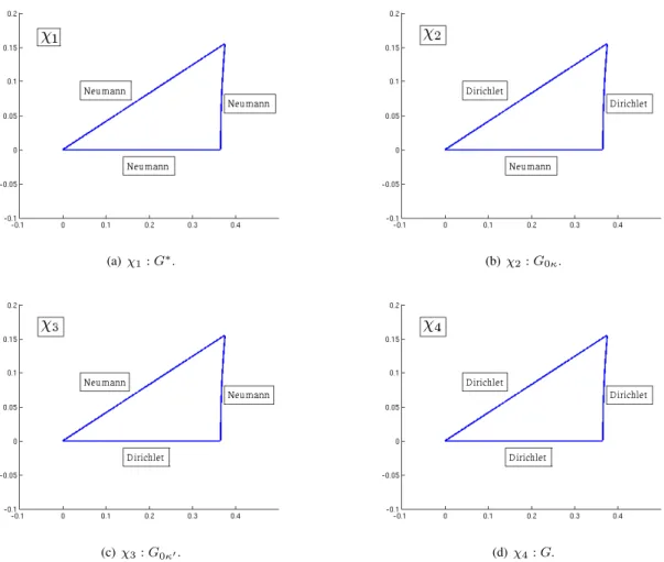
entails solving the eigenvalue problem in certain irreducible subregions of the fundamental domain, such as T (2, 3, 8), using special boundary conditions for these subregions. In effect the periodicity conditions in the original domain (octagon) may produce Dirichlet or Neumann conditions on the boundaries of these subregions. The symmetry groupG∗has a smaller fundamental domain, the triangleT (2, 3, 8) see figure1, which is 1
96th of
the original octagon. The method of desymmetrization can be applied to many other techniques than finite element methods (see [19]).
We now focus on the four one-dimensional irreductible representations(χi)i=1···4acting upon the generators
as indicated in table6. One can find in the book of F¨assler and Stiefel [19, Chapter 3] the principle of desym-metrization in the context of dihedral symmetry. We follow their method in the case of the symmetry groupG∗.
The first step is to attribute one number (value) to each of the 96 triangles that tesselate the octagon under the action ofG∗(see2), according to the character values obtained from table6, i.e.
±1 depending on the conjugacy class (remember we restrict ourselves to the one dimensional representationsχ1toχ4).
Let us take the example of the first irreductible representationχ1and explain how we obtain the domain and
the boundary conditions depicted in figure5. Table6shows that all 96 triangles end up with the same value, 1. This means that the eigenfunction we are looking for is even under all the 96 elements inG∗and it follows that it must
satisfy Neumann boundary conditions on all the edges of the tesselation of the hyperbolic octagon [4,2]. Finally, it is sufficient to solve the eigenproblem on the reduced domainT (2, 3, 8) with Neumann boundary conditions on its three edges. For the four one-dimensional representations one has to choose the correct combination of Neumann and Dirichlet boundary conditions as shown in figure5.
The representations of dimension≥ 2 require the same number of values as their dimension. For example there are two basis vectors determining the function values in the case of an irreductible representation of dimension 2. The table6is then no longer sufficient to set the values of the function on each triangles and one has to explicitly
write the matrices of the irreductible representation in order to obtain the suitable conditions. This is why we have restricted ourselves to the four one-dimensional representations as described in the previous paragraphs.
(a) χ1:G∗. (b) χ2:G0κ.
(c) χ3:G0κ�. (d) χ4:G.
Figure 5: Boundary conditions for the one-dimensional irreducible representations. Top left: boundary conditions for χ1, corresponding to the isotropy groupG∗. Top right: boundary conditions forχ2 corresponding to the
isotropy groupGOκ. Bottom left: boundary conditions forχ3corresponding to the isotropy groupG0κ�. Bottom
right: boundary conditions forχ4corresponding to the isotropy groupG.
5.2
Numerical experiments
As there exists an extensive literature on the finite element methods (see for an overview [13,1]) and as numerical analysis is not the main goal of this article, we do not detail the method itself but rather focus on the way to actually compute the eigenmodes of the Laplace-Beltrami operator.
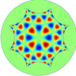
Desymmetrized problem : For the four problems depicted in figure5, we use the mesh generator Mesh2D from
Matlabto tesselate the triangleT (2, 3, 8) with 2995 nodes and we implement the finite element method of order 1. Our results are presented in figure6and are in a good agreement with those obtained by Balazs-Voros in [4] and Aurich-Steiner in [2]. Once we have computed the eigenfunction inT (2, 3, 8), we extend it to the whole octagon by applying the generators ofG∗. We superimpose in figure6(a)the tesselation of the octagon by the 96 triangles
in order to allow the reader to see the symmetry class ofG∗.
Non desymmetrized problem : As discussed previously, we also present some H-planforms of higher dimen-sion. We mesh the full octagon with 3641 nodes in such a way that the resulting mesh enjoys aD8-symmetry, see
(a) χ1 : G∗, the corrseponding eigenvalue is λ =
23.0790.
(b) χ2 : G0κ, the corrseponding eigenvalue is λ =
91.4865.
(c) χ3 : G0κ�, the corrseponding eigenvalue is λ =
32.6757.
(d) χ4 : G, the corresponding eigenvalue is λ =
222.5434.
Figure 6: The four H-planforms with their corresponding eigenvalue associated with the four irreductible repre-sentations of dimension 1, see text.