HAL Id: hal-02947769
https://hal.archives-ouvertes.fr/hal-02947769
Submitted on 8 Oct 2020
HAL is a multi-disciplinary open access
archive for the deposit and dissemination of
sci-entific research documents, whether they are
pub-lished or not. The documents may come from
teaching and research institutions in France or
abroad, or from public or private research centers.
L’archive ouverte pluridisciplinaire HAL, est
destinée au dépôt et à la diffusion de documents
scientifiques de niveau recherche, publiés ou non,
émanant des établissements d’enseignement et de
recherche français ou étrangers, des laboratoires
publics ou privés.
To cite this version:
A. Fortems-Cheiney, F. Chevallier, I. Pison, P. Bousquet, M. Saunois, et al.. The formaldehyde budget
as seen by a global-scale multi-constraint and multi-species inversion system. Atmospheric Chemistry
and Physics, European Geosciences Union, 2012, 12 (15), pp.6699-6721. �10.5194/ACP-12-6699-2012�.
�hal-02947769�
www.atmos-chem-phys.net/12/6699/2012/ doi:10.5194/acp-12-6699-2012
© Author(s) 2012. CC Attribution 3.0 License.
Chemistry
and Physics
The formaldehyde budget as seen by a global-scale
multi-constraint and multi-species inversion system
A. Fortems-Cheiney1, F. Chevallier1, I. Pison1, P. Bousquet1, M. Saunois1, S. Szopa1, C. Cressot1, T. P. Kurosu2, K. Chance3, and A. Fried4
1Laboratoire des Sciences du Climat et de l’Environnement, CEA-CNRS-UVSQ, UMR8212, Gif-sur-Yvette, France 2Jet Propulsion Laboratory, California Institute of Technology, USA
3Atomic and Molecular Physics Division, Harvard-Smithsonian Center for Astrophysics, Cambridge, Massachusetts, USA 4Earth Observing Laboratory, National Center for Atmospheric Research, Boulder, Colorado, USA
Correspondence to: A. Fortems-Cheiney ([email protected])
Received: 16 February 2012 – Published in Atmos. Chem. Phys. Discuss.: 7 March 2012 Revised: 4 July 2012 – Accepted: 5 July 2012 – Published: 1 August 2012
Abstract. For the first time, carbon monoxide (CO) and
formaldehyde (HCHO) satellite retrievals are used together with methane (CH4) and methyl choloroform (CH3CCl3 or
MCF) surface measurements in an advanced inversion sys-tem. The CO and HCHO are respectively from the MO-PITT and OMI instruments. The species and multi-satellite dataset inversion is done for the 2005–2010 period. The robustness of our results is evaluated by comparing our posterior-modeled concentrations with several sets of inde-pendent measurements of atmospheric mixing ratios. The in-version leads to significant changes from the prior to the pos-terior, in terms of magnitude and seasonality of the CO and CH4 surface fluxes and of the HCHO production by
non-methane volatile organic compounds (NMVOC). The latter is significantly decreased, indicating an overestimation of the biogenic NMVOC emissions, such as isoprene, in the GEIA inventory. CO and CH4 surface emissions are increased by
the inversion, from 1037 to 1394 TgCO and from 489 to 529 TgCH4on average for the 2005–2010 period. CH4
emis-sions present significant interannual variability and a joint CO-CH4fluxes analysis reveals that tropical biomass burning
probably played a role in the recent increase of atmospheric methane.
1 Introduction
Formaldehyde (HCHO), found throughout the troposphere, is a short-lived tropospheric gas acting as an outdoor and indoor air pollutant, with a typical lifetime of a few hours in daytime (Sander et al., 2006). HCHO is produced in the background troposphere mainly through the chemical oxi-dation of methane (CH4)by hydroxyl radicals (OH). In the
continental boundary layer, the HCHO source from the oxi-dation of non-methane volatile organic compounds NMVOC (i.e. alkanes, alkenes, aromatic hydrocarbons and isoprene) dominates over the methane oxidation source and can make a large contribution to tropospheric HCHO concentrations. HCHO is emitted into the atmosphere by fuel combustion processes, biomass burning (Lee et al., 1998) and vegetation (Lathi`ere et al., 2006), but with smaller contributions than oxidation. The major sinks of HCHO include oxidation by OH, two photolysis reactions, and dry and wet depositions.
Through its production and loss in the troposphere, HCHO is a key species in the oxidation chain of methane and of NMVOC, and can modulate the budget of carbon monox-ide (CO). However, very large uncertainties remain for the relative contributions of these different sources and sinks to the HCHO budget, particularly for the atmospheric produc-tion by NMVOC. This is mainly explained by the diversity of NMVOC, by their lifetimes varying from hours to weeks, and by the large spatio temporal variability of their emis-sions, leading to large uncertainties for the bottom-up esti-mates (that are based on emission factors or biogeochemical
for the improvement of emission inventories of HCHO and its precursors.
Complementary to bottom-up estimates, atmospheric in-version infers sources and sinks of atmospheric species by statistically tracing back atmospheric signals given by con-centration observations to the origin of emissions. It has played an important part during the last decade in the study of CH4 (e.g. Dentener et al., 2003; Bousquet et al., 2006;
Bergamaschi et al., 2009) and CO (P´etron et al., 2004; Pfis-ter et al., 2004; Heald et al., 2004; Tanimoto et al., 2008; Kopacz et al., 2010; Yurganov et al., 2010). Although chemi-cally coupled, the sources and sinks of these trace gases have often been optimized independently from each other. Alter-natively, Stavrakou and M¨uller (2006) have optimized CO emissions by taking into account their relation to NMVOC and HCHO through OH. Butler et al. (2005) performed a si-multaneous mass balance inversion of CH4 and CO
emis-sions at a low spatial resolution. Pison et al. (2009) im-plemented the Simplified Atmospheric Chemistry System (SACS) in a variational inversion system and demonstrated the feasibility of a multi-species inversion, inferring simulta-neously CH4, OH, H2, and CO sources and sinks. However,
these first studies did not use any HCHO observations. In-deed, large disagreements exist between the various measure-ment techniques employed for measuring HCHO mixing ra-tios (spectroscopic, chromatographic, and fluorimetric) (Hak et al., 2005). As a result, there is not yet a consistent global measurement network for HCHO as it exists for greenhouse gases or other air pollutants such as CO, CH4and ozone.
These limitations on the spatial coverage of the HCHO measurements can now be addressed by using HCHO to-tal columns retrieved by satellite, which offer the unique possibility of sensing atmospheric HCHO at a global scale. Even though uncertainties remain large for the HCHO satel-lite retrievals, past studies have demonstrated the usefulness of HCHO column data (determined in near-UV wavelengths 310–365 nm) from the Global Ozone Monitoring Experiment (GOME) (Abbot et al., 2003; Palmer et al., 2006, 2007; Fu et al., 2007; Barkley et al., 2008), from the SCanning Imag-ing Absorption spectroMeter for Atmospheric CartograpHY (SCIAMACHY) (Stavrakou et al., 2009) and from the Ozone Monitoring Instrument (OMI) (Millet et al., 2008; Marais et al., 2012) to constrain NMVOC emissions, the latter having the highest spatial resolution of these 3 instruments.
2003; Bousquet et al., 2005). This study provides an analy-sis of the global and regional HCHO budget, with a partic-ular focus on HCHO atmospheric production by NMVOC. In Sect. 2, the OMI and MOPITT satellite retrievals, and the surface measurements are briefly presented. Our chemical-transport model (described in Sect. 3) is forced by a complex flux scenario and used within an atmospheric inversion tech-nique to optimize HCHO sources and sinks against the en-semble of remote and surface data. The main characteristics of the inversion system are summarized in Sect. 4. Section 5 gives the results of the inversion and explores their main fea-tures in terms of HCHO budget and implications for the other species (OH, CO and CH4). The inverted HCHO and CO
sources are evaluated by comparison of the optimized and prior concentrations with independent (i.e. not used in the in-version) measurements from aircraft campaigns (INTEX-B, AMMA) and at the surface (NOAA/ESRL, AGAGE, CSIRO, EMPA, SAWS, NIWA and JMA/MRI).
2 Atmospheric constraints
2.1 OMI HCHO retrieved columns
The Ozone Monitoring Instrument (OMI) was launched aboard EOS Aura in July 2004. It has been flying on a 705 km sun-synchronous orbit that crosses the Equator at 13:38 LT. OMI is a near-UV/Visible nadir solar backscatter spectrom-eter covering the spectral range 270–500 nm with a resolu-tion of 0.45 nm between 310 and 365 nm. Its large swath of about 2600 km provides daily global coverage, with a spa-tial resolution of 13×24 km at nadir, increasing substanspa-tially across-track to give an average cross-track spatial resolution of ∼ 43 km. Measured trace gases include O3, NO2, SO2,
HCHO, BrO, and OClO (Levelt et al., 2006).
The level 2 data of OMI HCHO Version 3 total columns that we used have been collected from http://mirador.gsfc. nasa.gov/. The data selection follows the criteria of the data quality statement (NASA, 2008): only column values flagged as “good” in the product were included. Also, data with cloud fraction higher than 0.2 were excluded, as recommended by Millet et al. (2006), who showed that the bias on HCHO re-trievals decreases with decreasing cloud fraction (from 14 % at a cloud fraction of 0.4 to 6 % at a cloud fraction of 0.2). Similarly, only retrievals between 65◦S and 65◦N were used
in this study. Outliers (column > 1.0 × 10+19molec cm−2)
were also removed. OMI retrievals are affected by an artifi-cial drift, connected to an increase in detector dark current observed over OMI lifetime, from 2.72 × 10+15molec cm−2 in December 2004 to 8.05 × 10+15molec cm−2in December 2010. We have applied the empirical correction developed by the data providers. It should be noted that the total un-certainties of individual HCHO column retrievals typically range within 50–105 %, with the lower end of this range over HCHO hotspots (Kurosu, 2008).
Due to the scarcity of in situ HCHO measurements, op-portunities for validation have been so far limited. The OMI HCHO columns have been evaluated against GOME re-trievals by Millet et al. (2008) for the North American region. This study indicates a reasonable agreement between the two datasets: the OMI spatial distribution is similar to that ob-served by GOME in previous years (differences of 2–14 %), and OMI seems to exhibit less retrieval noise (as seen in their Fig. 2). Boeke et al. (2011) compared OMI HCHO columns to aircraft data over the USA, Mexico, and the Pacific, and found an average bias of less than 3 %.
2.2 MOPITT-V4 CO retrieved mixing ratios
The Measurements Of Pollution In The Troposphere (MO-PITT) instrument was launched aboard EOS Terra in Decem-ber 1999 and has been operating nearly continuously since March 2000. This spectrometer flies on a sun-synchronous orbit that crosses the Equator at 10:30 and 22:30 LT. The spatial resolution of its observations is about 22 km at nadir. Three days of measurements are needed to achieve global coverage with its 640-km swath.
The Level 2 data of MOPITT Version 4 have been col-lected from http://reverb.echo.nasa.gov/. They include CO mixing ratios at 10 standard pressure levels between the sur-face and 150 hPa for cloud-free spots. As a trade-off between data volume, closeness to the surface and retrieval noise, only the 700 hPa-level CO retrievals together with their associated averaging kernels (AK) were used here. Data within 25◦from the poles have been left out, as the weight of the a priori CO profile in the MOPITT retrievals increases towards the pole. MOPITT’s thermal band radiances are more sensitive to sur-face emissivity at night than during the day, and consequently less sensitive to the CO distribution at night (Crawford et al., 2004). Therefore, the CO retrieval errors are larger at night than during the day, and is why the nighttime observations have been excluded.
MOPITT retrievals have been evaluated on a regular basis since the start of the mission in 2000, and have been com-pared against aircraft measurements (made during the NASA INTEX-A, NASA INTEX-B and NSF MIRAGE field cam-paigns), as well as the long-term record from NOAA obser-vations and the MOZAIC experiment (Emmons et al., 2004, 2007, 2009). Retrieval errors are estimated to be about 10 % for each retrieval, with regional biases of a few parts per
bil-lion. The MOPITT retrievals suffer from a time-varying bias in Version 4 (Deeter et al., 2010), as in Version 3 (Yurganov et al., 2008; Emmons et al., 2009; Drummond et al., 2009). This positive bias drifts by about 0.5 ppbv yr−1, on average at 700 hPa, in Version 4 (Deeter et al., 2010). This positive bias drift is not taken into account in our observation error and may bias the inversion estimate. Nevertheless, the con-sistency of the MOPITT-based inverted fluxes with the IASI-based ones showed that the impact of the drift in the MOPITT retrievals is negligible (Fortems-Cheiney et al., 2011).
2.3 Methane and methyl chloroform surface observations
CO, HCHO, CH4and OH concentrations are chemically
re-lated. OH is an essential modulator of this reaction chain, but this short-lived compound (∼ 1 s) is not easy to constrain in a global atmospheric model. Our approach uses methyl chloroform (CH3CCl3or MCF) as a proxy tracer (Krol and
Lelieveld, 2003; Prinn et al., 2005; Bousquet et al., 2005). MCF only reacts with OH and its sources and sinks (emis-sions, photolysis, ocean sink) are assumed to be quantified with a rather good accuracy. During the target period of this study (2005–2010), Montzka et al. (2011) showed that the MCF proxy method gives comparable results to CTMs for OH variations. Here, OH monthly 3-D fields are optimized in four latitudinal volumes using a prior spatio-temporal dis-tribution of OH derived from a full chemistry climate model (Hauglustaine et al., 2004).
CH4 in situ measurements are also used to constrain
methane emissions. A set of stations that measured MCF and CH4, daily or nearly continuously for the 2005–2010 period,
has been selected from the AGAGE and NOAA/ESRL net-works available on the World Data Center for Greenhouse Gases site (WDCGG, http://ds.data.jma.go.jp/gmd/wdcgg/).
3 The LMDz-SACS chemistry transport model
LMDz-SACS is a global 3-D chemistry transport model (CTM) coupling an offline version of the atmospheric gen-eral circulation model LMDz (Hourdin et al., 2006) with the atmospheric chemistry module SACS (Simplified At-mospheric Chemistry System) (Pison et al., 2009). To min-imize the computational cost of the inversions, we use a pre-calculated archive of 3-hourly transport mass fluxes in-stead of running the full general circulation model LMDz. The archive has been obtained from a previous simula-tion of LMDz for the same dates, guided by the horizon-tal winds from ECMWF reanalyses. The horizonhorizon-tal resolu-tion is 3.75◦×2.75◦and the vertical resolution includes 19 sigma-pressure levels (first level thickness of about 150 m, resolution in the boundary layer of 300 to 500 m and ≈ 2 km at tropopause). SACS is a very simplified version of INCA (INteraction Chimie A´erosols, Hauglustaine et al., 2004;
HCHO + OH(+O2) →HO2+CO + H2O
k =1.50 × 10⁻¹³exp(1.06P /Po) cm3molec−1s−1 (3) HCHO + hν(+O2) →H2+CO
Jprecomputed by INCA (4)
HCHO + hν(+O2) →2HO2+CO
Jprecomputed by INCA (5)
The prior sources and sinks of formaldehyde, entering or cal-culated by LMDz-SACS, are summarized in the schematic Fig. 1a), which also depicts part of the SACS mechanism. Averaged over the 6-yr period, the prior photochemical de-struction of HCHO is 1210 TgHCHO yr−1 and the surface wet and dry deposition account for 32 TgHCHO yr−1. We as-sume that methane is oxidized into HCHO in a single step, thereby neglecting the formation of methyl hydroperoxide under low NOx conditions, which can delay or slightly
re-duce the HCHO atmospheric production. The global prior HCHO atmospheric production is 1332 TgHCHO yr−1, with a contribution of 974 TgHCHO yr−1 from methane oxida-tion and a contribuoxida-tion of 358 TgHCHO yr−1from NMVOC
oxidation. Indeed, in addition to the photochemical reac-tions shown above, the source of HCHO from the degra-dation of NMVOC is prescribed in SACS. This 3-D pro-duction of formaldehyde is obtained from a previous sim-ulation of the full atmospheric chemistry model LMDz-INCA using NMVOC emissions and chemistry of Folberth et al. (2006). In this full-chemistry simulation, the anthro-pogenic NMVOC emissions were those from the Emission Database for Global Atmospheric Research (EDGAR-v3.2, http://edgar.jrc.ec.europa.eu) database valid for 1995 (Olivier and Berdowski, 2001); the biogenic NMVOC and formalde-hyde emissions were taken from the Global Emissions In-ventory Activity (GEIA) database (Guenther et al., 1995). Biomass burning emissions were from the interannual Global Fire and Emission database GFED-v2 (van der Werf et al., 2006) (http://www.globalfiredata.org/).
The sources of the other species, CO and CH4,
includ-ing industry and fossil fuel combustion, are drawn from the EDGAR-v3.2 and from GFED-v2 inventories. The emissions of CH4due to wetlands and termites are based on the study of
Fung et al. (1991). It should be noted that we did not adapt the 1995 EDGAR-v3.2 inventory to the 2000s. We choose EDGAR-v3.2 rather than the recent EDGAR-v4.2 for con-sistency with the study of Fortems-Cheiney et al. (2011).
Fig. 1. Prior (a) and posterior (b) HCHO sources and sinks in the
SACS mechanism. Sinks of H2and the HCHO deposition are
in-cluded in SACS but not displayed. Changes of arrow thickness be-tween prior and posterior indicate a reduction or an increase of the sources and sinks. Values are for year 2006.
4 The inverse model
Our inverse problem consists in optimizing the 3-D atmo-spheric production of formaldehyde, the surface emissions of CO and CH4, and OH concentrations within the same
inver-sion. We apply the inverse method described by Chevallier et al. (2005, 2007). This inversion scheme uses the LMDz-SACS adjoint model developed by Pison et al. (2009). The optimal solution (in a statistical sense) is found by iteratively minimizing the following cost function:
J (x) = (x − xb)TB−1(x − xb) + (H (x) − y)T
R−1(H (x) − y), (6)
where x is the state vector that contains the variables to be optimized by the inversion:
– CO, CH4, and MCF surface emissions at a 3.75◦×2.5◦
(longitude, latitude) resolution.
– CO, CH4, and MCF 3-D initial conditions at an 8-day
and at a 3.75◦×2.5◦resolution.
– 2-D factors to scale the 3-D-chemical production of
HCHO (due to NMVOC) at an 8-day and 3.75◦×2.5◦ resolution.
– 4 factors to scale the OH atmospheric concentrations for
each 8-day period within four latitude bands (90–30◦S, 30◦S–0, 0–30◦N, 30–90◦N).
The prior information xb is a combination of the datasets EDGAR-v3.2, GFED-v2 and GEIA, as described in Sect. 3. The error statistics have been detailed in Fortems-Cheiney et al. (2011) and their main features are recalled here. The covariance matrix B of the prior errors is defined as diago-nal. The error standard deviations assigned to the CO prior
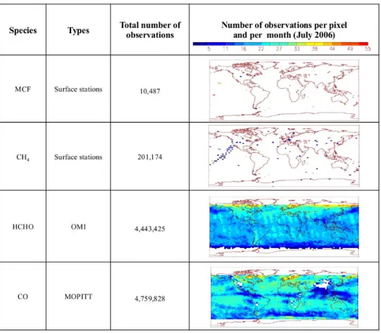
Fig. 2. Summary of the observations used in the inversion: total number of observations over the 2005–2010 time period and typical
distri-butions of these observations on the right for July 2006.
emissions in the covariance matrix B are set at 100 % of the maximum value of the emission time series during the corre-sponding year for each grid point. The choice of a relatively large value accounts for uncertainties in the seasonal cycle of particular emissions, such as fires (Chevallier et al., 2009). Given the large discrepancies associated with the biogenic NMVOC estimates (i.e. between IPCC, 2001 and Guenther et al., 2006), errors assigned to the scaling factors of the 3-D-chemical production of HCHO are set to 400 %. For MCF emissions, the EDGAR-v3.2 inventory by Olivier et al. (2001) has been adapted to give estimates of MCF emis-sions over our time period (2005–2010) by applying an expo-nential decrease (update of Bousquet et al., 2005). As MCF emissions are well known, errors are set to 1 % of the flux for MCF. The errors assigned to the scaling factor of OH are set to 10 %, based on the differences seen between various estimates of OH concentrations (Prinn et al., 2001; Krol and Lelieveld, 2003; Bousquet et al., 2005). Finally, errors are set to 100 % of the flux for CH4. Several sensitivity tests
associ-ated with these prior settings are presented in Sect. 6. For the initial conditions, errors are set to 10 % for HCHO and MCF and to only 3 % for CH4 and 5 % for CO.
Spa-tial correlations are defined by an e-folding length of 500 km
over land and 1000 km over sea, without any correlation be-tween land and ocean grid points. Temporal correlations are neglected.
The observations vector y used for the inversion are sur-face observations of MCF and CH4, as well as satellite
re-trievals from MOPITT for CO, and from OMI for HCHO (see Sect. 2), both averaged into “super-observations” at the 3.7◦×2.75◦resolution of LMDz-SACS, amounting to about 9.5 million for the 2005–2010 time period (see the distribu-tion in Fig. 2). For MOPITT, as the averaging kernel (AK) profiles do not vary much within the grid cell, we use the AK profile of the first retrieval when several of them are averaged into a super-observation. No averaging kernels are available for the OMI product; the calculation of HCHO columns is performed as a mean, weighted by the relative thickness of model pressure layers.
Error correlations between the super-observations are ne-glected, so that the covariance matrix R of the observation errors is diagonal (i.e. only variances are taken into ac-count). The diagonal R-matrix representing observation rors is filled with variances which combine representation er-rors (e.g. the mismatch between the observation and model resolutions), errors of the observation operator (including
Figure 3. Definition of the14 regions used in this study.
1014
Fig. 3. Definition of the 14 regions used in this study.
transport and chemical-scheme errors in LMDZ-SACS) and measurements errors. The errors of the observation opera-tor and the representation error are difficult to estimate pre-cisely. LMDz-SACS accumulates the errors of the reference model LMDz-INCA, complemented by those due to the sim-plifications made in the chemical scheme. As a consequence, we chose to define the variance of the individual observation errors in R as the quadratic sum of the measurement error reported in the MOPITT and the OMI data sets, and of the CTM errors set to 50 % of the retrieval values following Pi-son et al. (2009).
The 6-yr period considered here is processed in a single in-version. The presence of OH among the optimized variables makes the H operator diverge from linearity and makes the cost function J diverge from quadracity. In this context, the cost function and the norm of its gradient are minimized with the quasi-Newton minimization algorithm M1QN3 (Gilbert and Lemar´echal, 1989), and our system is adapted to deal with non-linearities. After 28 iterations, corresponding to 5 weeks of calculation on 8 processors, the norm of the gradi-ent of the cost function is reduced by 98 %. More iterations do not further reduce the norm of the gradient.
As described by Chevallier et al. (2007), it is possible to rigorously compute the uncertainty of the inverted fluxes by a Monte-Carlo approach. Because of its large computational expense, the computation of the uncertainty on the inverted fluxes was performed for year 2006 only. This results in a sta-tistical ensemble of 48 realizations of weekly fluxes, in which the prior and the observations follow their respective error statistics. This ensemble allows computing the flux uncer-tainty reduction up to the monthly scale. Here, the monthly flux uncertainty reduction is assumed to be about the yearly flux uncertainty reduction for HCHO and for CO because of the relatively short lifetime of these species, but this assump-tion does not hold for CH4, whose lifetime is about 12 yr
(IPCC, 2007). In the following, error bars will therefore be given for HCHO and for CO only.
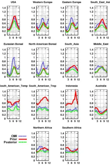
Fig. 4. Times series of monthly averaged formaldehyde total
columns retrieved by OMI (in blue) and simulated by the model LMDz-SACS using the prior (in red) and the posterior fluxes (in green) for year 2006, from January to December. Error bars repre-sent the OMI retrieval errors. Units are 10e16molec cm−2.
5 Results
Figure 3 shows the 14 continental regions used to analyse our results.
5.1 Prior and posterior HCHO total columns, and fit to OMI observations
The OMI observations, the prior, and the posterior-modeled monthly mean global HCHO columns averaged over the 14 continental regions are shown in Fig. 4 for year 2006. The HCHO prior columns simulated by the model weakly agree with OMI observations, both in magnitude and in their seasonal cycle. Except over the two boreal and Euro-pean regions, OMI measurements are smaller than the prior columns for the entire year. The largest discrepancies are found over the tropical regions, and particularly over South America and Indonesia. This has already been pointed out by Barkley et al. (2008), who found higher model HCHO
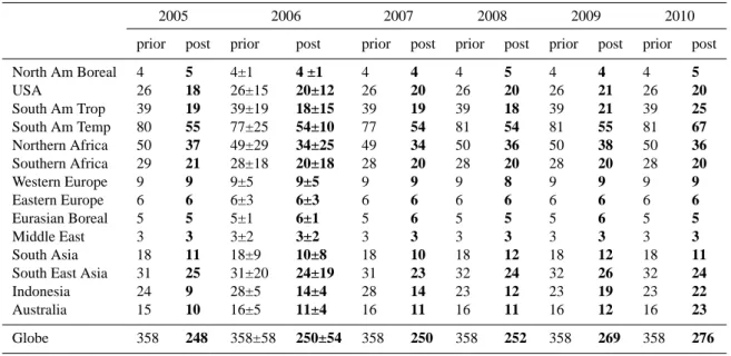
Table 1. Total 3-D HCHO production by NMVOC for years 2005 to 2010 before inversion and after inversion, for 14 continental regions and
for the globe in TgHCHO yr−1. All budgets correspond to a 12-month period. The uncertainty of the inverted fluxes for 2006 are computed
by a Monte-Carlo approach.
2005 2006 2007 2008 2009 2010
prior post prior post prior post prior post prior post prior post
North Am Boreal 4 5 4±1 4 ±1 4 4 4 5 4 4 4 5 USA 26 18 26±15 20±12 26 20 26 20 26 21 26 20 South Am Trop 39 19 39±19 18±15 39 19 39 18 39 21 39 25 South Am Temp 80 55 77±25 54±10 77 54 81 54 81 55 81 67 Northern Africa 50 37 49±29 34±25 49 34 50 36 50 38 50 36 Southern Africa 29 21 28±18 20±18 28 20 28 20 28 20 28 20 Western Europe 9 9 9±5 9±5 9 9 9 8 9 9 9 9 Eastern Europe 6 6 6±3 6±3 6 6 6 6 6 6 6 6 Eurasian Boreal 5 5 5±1 6±1 5 6 5 5 5 6 5 5 Middle East 3 3 3±2 3±2 3 3 3 3 3 3 3 3 South Asia 18 11 18±9 10±8 18 10 18 12 18 12 18 11
South East Asia 31 25 31±20 24±19 31 23 32 24 32 26 32 24
Indonesia 24 9 28±5 14±4 28 14 23 12 23 19 23 22
Australia 15 10 16±5 11±4 16 11 16 11 16 12 16 23
Globe 358 248 358±58 250±54 358 250 358 252 358 269 358 276
columns (using the GEOS-Chem chemistry-transport model and the MEGAN inventory for NMVOC emissions) than GOME HCHO measurements. HCHO concentrations are mainly driven by NMVOC emissions and the uncertainties associated with these NMVOC emissions (e.g. in the GEIA inventory, or in Model of Emissions of Gases and Aerosols MEGAN) are large (Barkley et al., 2008). These uncertain-ties result from errors in emission factors, and from incor-rect or incomplete parameterizations of activity factors. For example, tropical rainforest emission in the GEIA inventory are based on ambient isoprene concentration measurements from a single study (Zimmerman et al., 1988; Barkley et al., 2008), which could explain the notable differences in terms of magnitude over tropical regions.
In tropical regions, except Indonesia, our prior does not re-produce the observed seasonal cycle, particularly over South America and Africa. It should be noted that the entire grow-ing season of isoprene emission is represented by a sgrow-ingle basal emission factor in GEIA inventory. Kuhn et al. (2004) found it inadequate for certain representative tropical plant species. This could explain the differences in terms of sea-sonality over tropical regions.
After optimization of the 3-D HCHO production, the model succeeds in capturing both the seasonal cycle and the magnitude of the concentrations. Indeed, Fig. 4 shows a better fit than between the posterior simulated columns and the observations compared to the prior ones over re-gions USA, South Asia, South East Asia, Australia, South American Temperate, South American Tropical and Indone-sia. However, some discrepancies remain: for example, the model fails to reproduce the observed seasonal decrease from
July to October over North Africa. This could be explained by the relatively large OMI data uncertainties over this region (particularly over Sahara), reaching more than 250 %, which implies less deviation from prior fluxes as compared to re-gions with less uncertain data. The agreement for the two boreal regions is not as good as for other regions because OMI data north of 65◦N are not used in the inversion.
5.2 Optimization of the HCHO sources and sinks
The optimization of the HCHO column implies changes in the HCHO sources and sinks (surface emissions, atmospheric production and atmospheric loss), which are displayed in Fig. 1b. We do not consider changes of the HCHO surface emissions in the following, as they are very small in magni-tude compared to the atmospheric production and loss.
5.2.1 Prior and posterior 3-D HCHO production by NMVOC
As HCHO is produced by NMVOC oxidation, and as some NMVOC have sufficiently short lifetimes, there exists a re-lationship at local scale between the emission of NMVOC, their oxidation into HCHO and the observed HCHO column. As a result, the 3-D HCHO production by NMVOC is a good indicator for the emissions of short-lived NMVOC (Palmer et al., 2003). The prior and posterior HCHO productions by NMVOC are shown in Table 1 and in Fig. 5.
The posterior global 6-yr average HCHO production by NMVOC is estimated at 257 TgHCHO yr−1, about 28 % smaller than the prior estimate (358 TgHCHO yr−1, Fig. 1b and Table 1). All regions contribute to this decrease but the
Fig. 5. Times series of prior (in blue) and posterior (in red)
HCHO 3-D production by NMVOC for year 2006. Units are TgH-CHO/month.
changes are smaller for Europe, Middle East and for the two boreal regions. The main changes are seen over regions of high NMVOC emissions (De Smedt et al., 2008): the USA and South Asia in the Northern Hemisphere, and all tropical regions. We discuss our results for these particular regions in the following.
Regional budget and comparison with recent studies
The annual posterior 3-D HCHO production by NMVOC is decreased by 26 % over the USA, from 26 TgHCHO to 19 TgHCHO on the 6-yr average. As seen in Fig. 5, this de-crease only affects the summer months, dominated by en-hanced isoprene emissions. Indeed, recent studies (Abbot et al., 2003; Palmer et al., 2003, 2006; M¨uller et al., 2008) showed that the variability of the HCHO columns over North America reflects the emissions of NMVOC precursors, and particularly isoprene. Consequently, our results suggest a large overestimation of isoprene emissions over the USA in the GEIA inventory. This is in agreement with the study of Stavrakou et al. (2009). They evaluated the accuracy of
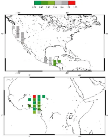
Fig. 6. Ratio of the posterior to the prior values of bias (in
abso-lute value) between simulated and observed concentrations for the INTEX-B (top) and AMMA campaigns (bottom). The inversion im-proves the simulation when the ratio of the absolute bias is less than 1 (in green).
the GEIA biogenic emission inventory (502 Tg yr−1for iso-prene, 127 Tg yr−1 for terpenes, as used in this study) and the Model of Emissions of Gases and Aerosols MEGAN-ECMWF (M¨uller et al., 2008) against a new dataset of spaceborne HCHO columns derived from GOME and SCIA-MACHY. When they halved the isoprene emissions of the MEGAN-ECMWF inventory over North America (similar to the GEIA’s inventory in this particular region), they ob-tained a significant reduction of their observation to model bias (from 37.2 to 7.6 %). Also, the isoprene emissions in-ferred by Palmer et al. (2003) from the GOME data are 20 % less than those of GEIA. Shim et al. (2005) recently inverted global isoprene emissions for various ecosystems from September 1996 to August 1997 using the GOME formaldehyde measurements. They found isoprene emission budgets 14 % smaller than those of GEIA over the USA, with a reduction for particular ecosystems (grass/shrub, dry ever-green, crop/woods, and the regrowing woods).
In South Asia, the posterior 3-D HCHO production by NMVOC is almost half the prior, estimated at 11 TgHCHO compared to the prior 18 TgHCHO. Figure 5 shows that the prior and the posterior HCHO production by NMVOC are in
a reasonable agreement in January and in December for this region when the most abundant source is attributed to anthro-pogenic activities and particularly to strong domestic heating (Fu et al., 2007). However, for the rest of the year, the pos-terior HCHO source from NMVOC is significantly smaller than the prior one. Also, the HCHO production by NMVOC is decreased during the growing season, from April to Oc-tober. This feature also points to an overestimation of the biogenic NMVOC emission, such as isoprene, in the GEIA inventory. In Indonesia, the posterior 3-D HCHO production by NMVOC is largely decreased by the inversion (−54 %), from 26 to 12 TgHCHO on the 6-yr average.
The African continent has a posterior 3-D HCHO produc-tion by NMVOC of 54 TgHCHO (34 TgHCHO for Northern Africa and 20 TgHCHO for Southern Africa), 36 % smaller than the prior one. This value is in agreement with the study of Marais et al. (2012), who inferred isoprene emissions from HCHO OMI satellite data and applied it to the African conti-nent: they found total OMI-derived isoprene emissions 22 % smaller than MEGAN (60 vs. 77 TgC yr−1), and concluded that isoprene emissions are overestimated over the central African rainforest in their prior inventory.
Finally, the inverse modeling results also suggest a much lower HCHO production by NMVOC for regions South American Tropical and South American Temperate, by re-spectively 51 % and 31 %. Their total posterior HCHO pro-duction by NMVOC sources is 19 and 54 TgHCHO on the 6-yr average. In these two regions, it is difficult to separate the biomass burning and biogenic NMVOC contributions to the observed HCHO signal. However, it can be noticed that Shim et al. (2005) found posterior isoprene emissions 30 % smaller than the corresponding GEIA estimate for South America, with a large reduction of the tropical rain forest emissions. The MEGAN-ECMWF biogenic fluxes averaged over the 1997–2011 period are also lower than the GEIA inventory by 40 % (62 vs. 87 TgC yr−1) (Stavrakou et al., 2009).
Seasonality and interannual variability
Figure 5 shows the time series of the prior and posterior monthly 3-D HCHO production by NMVOC in each re-gion. There are some interesting differences in seasonality between prior and posterior cycles. Over tropical regions (ex-cept Indonesia), the optimization dramatically changes the seasonal cycle. For example, the posterior cycles over North-ern Africa present two peaks (in September and in April) in both the wet and dry seasons, with highest values dur-ing the dry season. Over region South American Tropical, instead of peaking at 4.2 TgHCHO in August only like the prior, the posterior estimates peak at 2 TgHCHO in April (wet season) and at 2.1 TgHCHO in September (dry season). Interestingly, this posterior seasonal cycle agrees well with the in-situ tower measurements of isoprene, also showing
two peaks, made for year 2002 at Tapajos National Forest in Brazil (Barkley et al., 2008, their Fig. 8).
The annual 3-D HCHO production ranges between 248 TgHCHO yr−1 (in 2005) and 276 TgHCHO yr−1 (in 2010), showing a slight interannual variability (IAV). Table 1 shows the regional variation of the 3-D HCHO production by NMVOC between 2005 and 2010: tropical regions (South American Temperate, South East Asia, Northern Africa and Indonesia) are the main contributors to this IAV.
Theoritical uncertainty reduction
The Bayesian prior and the posterior uncertainties (1σ ) on the 3-D HCHO production by NMVOC are presented in Ta-ble 1 for year 2006. By reducing the uncertainty, the inver-sion also improves the quality of the 3-D HCHO produc-tion by NMVOC estimates (Table 1). The uncertainty re-duction is maximal in the regions South American Temper-ate (27 %), USA (20 %), South American Tropical, Northern Africa (14 %) and Indonesia (14 %). Significant reductions are also observed for other regions (e.g. 8 % in Western Eu-rope). There is no error reduction in the two boreal regions (North American Boreal and Eurasian Boreal) due to the lack of OMI data north of 65◦N.
5.2.2 Prior and posterior HCHO production by methane
As the formaldehyde production by methane via the reaction with O1D is very small (1 % of the global total), we only fo-cus on the HCHO production by methane via the oxidation by OH. The global prior HCHO production by methane is estimated at 967 TgHCHO yr−1on the 6-yr average. Because
of the small uncertainties prescribed on prior MCF emissions and MCF observations constraining the OH concentrations (and consequently the loss of methane), the posterior HCHO production by methane is only 2 % smaller than the corre-sponding prior (946 TgHCHO yr−1). No change is observed over the regions South American Temp, Middle East, Aus-tralia, Indonesia and the USA. The other regions see their HCHO production decrease only a few percentage points (i.e.
−3 % for South East Asia) (not shown).
5.2.3 Prior and posterior HCHO loss
The global posterior HCHO loss is estimated at 1181 TgHCHO yr−1, 8 % smaller than the
correspond-ing prior of 1296 TgHCHO yr−1on the 6-yr average. As a
consequence of the reduction of the NMVOC source, the main changes are seen only for regions that are impacted by the inversion in terms of HCHO production by NMVOC (Fig. 5): USA, South Asia and tropical regions.
Fig. 7. Seasonal cycle of the global tropospheric mean of OH prior concentrations from LMDz-INCA (in red), OH posterior concentrations
using only MOPITT as constraints from Fortems-Cheiney et al. (2011) (in blue) and OH posterior concentrations using OMI, MOPITT and surface stations (this study, in green), from January 2005 to December 2010. Units are mol cm−3.
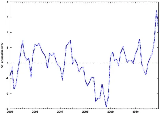
Fig. 8. Anomalies in global OH concentrations derived in our inversion from January 2005 to December 2010. Units are %.
5.3 Evaluation with independent data
We evaluate the multi-constraint system’s performance by comparing our posterior-modeled HCHO concentrations with independent observations. Considering that OMI data
integrate the atmospheric column of HCHO, comparison with aircraft observations are of particular interest. The air-borne HCHO measurements made during INTEX-B (Inter-continental Chemical Transport Experiment B) (Singh et al., 2009; Fried et al., 2011) and AMMA (African Monsoon
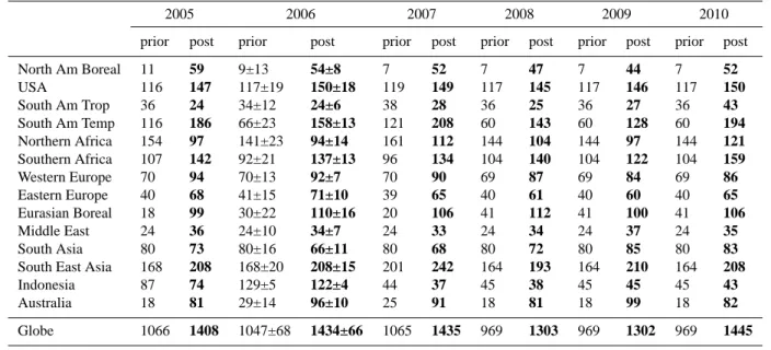
Table 2. Total CO emissions for years 2005 to 2010 before inversion and after inversion, for 14 continental regions and for the globe in
TgCO yr−1. All budgets correspond to a 12-month period. The total estimates include an oceanic CO source amounting to 20 TgCO yr−1.
The uncertainty of the inverted fluxes for 2006 are computed by a Monte-Carlo approach.
2005 2006 2007 2008 2009 2010
prior post prior post prior post prior post prior post prior post
North Am Boreal 11 59 9±13 54±8 7 52 7 47 7 44 7 52 USA 116 147 117±19 150±18 119 149 117 145 117 146 117 150 South Am Trop 36 24 34±12 24±6 38 28 36 25 36 27 36 43 South Am Temp 116 186 66±23 158±13 121 208 60 143 60 128 60 194 Northern Africa 154 97 141±23 94±14 161 112 144 104 144 97 144 121 Southern Africa 107 142 92±21 137±13 96 134 104 140 104 122 104 159 Western Europe 70 94 70±13 92±7 70 90 69 87 69 84 69 86 Eastern Europe 40 68 41±15 71±10 39 65 40 61 40 60 40 65 Eurasian Boreal 18 99 30±22 110±16 20 106 41 112 41 100 41 106 Middle East 24 36 24±10 34±7 24 33 24 34 24 37 24 35 South Asia 80 73 80±16 66±11 80 68 80 72 80 85 80 83
South East Asia 168 208 168±20 208±15 201 242 164 193 164 210 164 208
Indonesia 87 74 129±5 122±4 44 37 45 38 45 45 45 43
Australia 18 81 29±14 96±10 25 91 18 81 18 99 18 82
Globe 1066 1408 1047±68 1434±66 1065 1435 969 1303 969 1302 969 1445
Multidisciplinary Analysis) (Reeves et al., 2010; Borbon et al., 2012) are used for this comparison. The INTEX-B data have been collected in March–May 2006 from aircrafts flying across Mexico and the Gulf Coast of the USA (4–22 March) and across the Pacific Ocean and the western coastal regions of the USA (17 April–15 May). We compute the ratio of the posterior to the prior bias between modeled and observed concentrations. Locations highlighted in green in Fig. 6, for which ratio is lower than 1, show an improvement of the corresponding statistical indicator after optimization. Over Mexico, the mean bias is reduced by about 4 % (from 2.6 to 2.5 ppb) after the inversion. However, as the prior and pos-terior simulated concentrations are both in a good agreement with the observations over the USA in March (Fig. 4), target period of the INTEX-B campaign, the ratios of the posterior to the prior bias only range from 0.88 to 1.01 over the Pacific Ocean and the western coastal regions of the USA (Fig. 6, top).
The airborne campaigns AMMA were carried out in August 2006, when the monsoon season was fully devel-oped, across Niamey (Niger). With significant modifica-tions in terms of magnitude (monthly mean value of about 1.5 TgHCHO for the posterior, against about 3 TgHCHO for the prior) and in terms of seasonal variations (with peaks both in the wet and dry season) over Northern Africa, the inver-sion leads to a dramatic improvement relative to the prior over the Niger, Benin, and Ghana (see Fig. 6, bottom), with a reduction of the mean bias (data minus model) by about 40 % (from 3 to 1.8 ppb).
5.4 Implications for the other species 5.4.1 OH concentrations
Figure 7 compares the global tropospheric mean of OH concentration between the prior from the full chemistry-climate LMDz-INCA model (in red), the posterior derived from Fortems-Cheiney et al. (2011) (using the same inversion framework over the same period, but with only MOPITT-CO satellite data as constraints) and from this study for the period 2005–2010. From this study, the global OH posterior concen-tration value is 8.69×10⁵mol cm−3on average, 17 % smaller than the 10.5 × 10⁵mol cm−3 value of Prinn et al. (2005), and 1.6 % higher than the 8.55 × 10⁵mol cm−3of
Fortems-Cheiney et al. (2011). Figure 8 shows the OH concentration anomalies over the period 2005–2010, relative to the mean. The interannual variability is less than ± 4 %, consistent with the low variations reported in Montzka et al. (2011) and com-patible with the small IAV inferred by chemistry transport models (Dentener et al., 2003).
5.4.2 CO surface emissions and atmospheric production
The prior and posterior CO surface emissions are presented in Table 2 with their respective uncertainties (1σ ) for year 2006. Posterior CO emissions and production from Jan-uary 2005 to December 2010 reveal higher surface emis-sions (with contribution of all the regions except Northern Africa, South American Tropical, Indonesia and South Asia), and reduced atmospheric production than the prior estimates (Fig. 1b). The posterior emissions, with a global 6-yr average
Some regions show a very similar budget between MOPITT-OMI and MOPITT inversions: South Africa (142 and 149 TgCO yr−1 in 2005) and Australia (81 and 78 TgCO yr−1in 2005). However, there are some differences on emissions (e.g. for the USA with +11 %) due to the decrease of the CO tropospheric production over these re-gions. In our previous work with “MOPITT-only” inversion, we found CO emissions of 127 TgCO yr−1, much higher
than Kopacz et al. (2010) results (46.5 TgCO yr−1). Here, the differences between our model and Kopacz et al. (2010) are increased as posterior emissions of 147.5 TgCO yr−1are found. The cause of such a difference is still unclear. How-ever, our value of 206 TgCO yr−1 for North America (6-yr average) is in agreement with Hooghiemstra et al. (2012) who found 208 TgCO yr−1and 202 TgCO yr−1(inverted re-spectively with NOAA stations and with MOPITT for year 2004, their Table 1).
On the contrary, we notice that the “MOPITT-OMI”-based emissions are much smaller than the “MOPITT-only”-based ones in the Middle East region (−50 %, from 75 to 36 TgCO yr−1) and may be more realistic given the
rela-tively small size of the region and its emission profile. This surface emission decrease is compensated by an increase of the CO atmospheric source. Region South East Asia re-gion also sees its emissions decrease (by 19 %, from 274 to 208 TgCO yr−1), reaching a better agreement with the op-timized value of 207 TgCO yr−1 from P´etron et al. (2004) and of 169–228 TgCO yr−1 from Carmichael et. (2003). This modification is allowed by a better fit of the posterior simulated concentrations to the MOPITT observations (not shown).
Interannual variability
In terms of IAV, mostly explained by changes in biomass burning emissions and climate (Szopa et al., 2007; van der Werf et al., 2008, 2010), it should be noted that there is no noticeable change between this study and the work of Fortems-Cheiney et al. (2011). The lowest estimation of an-nual CO emissions is seen for years 2008 and 2009 with 1303 and 1302 TgCO yr−1, respectively. The highest emis-sions of the 2005–2010 period are seen for year 2010 (with 1445 TgCO yr−1, 10 % higher than the 2009 estimation.), followed by year 2007 (with 1435 TgCO yr−1) and year 2006 (with 1434 TgCO yr−1).
+50 TgCO, respectively, between 2006 and 2007). For South East Asia, it should be noted that the 2007 biomass burning emissions (particularly the peak in March) were extremely high, whereas the biomass burning emissions in the other years could be considered as normal (Fortems-Cheiney et al., 2011).
After low value in 2006 (158 TgCO yr−1) related to
unfavorable climate conditions (Gloudemans et al., 2009; Schroeder et al., 2009), there was a peak in CO emissions in 2007 (208 TgCO yr−1) over the region South American Temperate, correlated with the largest number of fires de-tected from space over the last 10 yr (Torres et al., 2010). In 2008 and 2009, the CO emissions show a negative trend with, respectively, 143 TgCO yr−1 and 128 TgCO yr−1. However, CO emissions returned to high levels in 2010. This increase is explained by the Amazon drought, co-occuring with peaks of fire activity (Lewis et al., 2011) and higher biomass burning emissions in the South American Temperate region (+66 TgCO between 2009 and 2010).
Theoritical uncertainty reduction
The prior and the posterior uncertainties (1σ ) on the CO emissions are presented in Table 2 for year 2006. The uncer-tainty reduction is maximal for the South American regions (46 % and 43 %, respectively, for South American Tropical and South American Temperate), and for Western Europe (43 %).
Evaluation with independant data and impact of the ad-ditional constraints
The posterior “MOPITT-OMI” emissions are evaluated for year 2006 by comparing the prior and the posterior mod-eled CO concentrations with independent (i.e. not used in the inversion) and fixed surface measurements from various networks (NOAA/ESRL, AGAGE, CSIRO, EMPA, SAWS, NIWA and JMA/MRI) available on the WDCGG website. We have restricted our analysis to 39 sites (33 in the Northern Hemisphere presented in Table 3 and 6 at the high-latitudes of the Southern Hemisphere presented in Table 4) represent-ing remote areas (i.e. Barrow, South Pole), or on the contrary, stations close to source regions (i.e. Jungfraujoch, Sonnblick,
Table 3. Statistics of the fit for the 33 stations chosen in the Northern Hemisphere. Bias is defined as the mean difference between observed
and modeled CO concentrations (model-minus-observation, average over the year 2006). The “MOPITT-only posterior” bias is given by Fortems-Cheiney et al. (2011). The lowest bias for each station is highlighted in bold.
Biais [ppb]
Code Location Prior Posterior MOPITT-only
posterior
ALT Alert, Canada −25.8 17.0 13.1
ASC Ascension Island, UK −7.7 −0.6 −0.7
ASK Assekrem, Algeria −18.9 −10.1 −6.4
AZR Terceira Island, Portugal −29.8 −9.2 −7.7
BMW Tudor Hill, IK −12.5 −11.7 12.5
BRW Barrow, USA −28.5 20.3 17.5
BSC Black Sea, Romania −38.7 4 3.6
CBA Cold Bay, USA −33.6 11.2 10.8
CHR Christmas Island, Kiribati −7.8 −5.5 −5.7
EIC Easter Island, Chile −9.0 2.1 1.3
GMI Mariana Islands, Guam −23.6 −16.4 −13.8
ICE Heimay, Iceland −23.7 10.4 7.6
IZO Izana, Spain −23.7 −13.8 −10.0
JFJ Jungfraujoch, Switzerland −24.9 −0.4 −23
KUM Cape Kumukahi −24.1 −7.3 −8.2
KZM Plateau Assy, Kazakhstan −22.5 11.4 17.8
MHD Mace Head, Ireland −25.0 3.3 4.3
MID Sand Island, USA −24.8 −12.4 −12.9
MLO Mauna Loa, USA −32.6 −16.8 −14.6
MNM Minamitorishima, Japan −15.1 −2.4 −6.1
NWR Niwot Ridge, USA −30.4 −11.6 −9.2
PAY Payerne, Switzerland −54.7 −10.4 −19.5
RIG Rigi, Switzerland −14.2 23.3 19.0
RPB Ragged Point, Barbados −15.9 −8.7 −5.5
RYO Ryori, Japan −44.1 11.7 20.5
SEY Mahe Island, Seychelles −5.2 −6.3 3.2
SHM Shemya Island, USA −32.7 3.1 3.8
SNB Sonnblick, Austria −77.2 52.5 −54.8
SMO Cape Matatula, American Samoa −6.6 −0.8 −0.2
UUM Ulaan Uul, Mongolia −29.1 25.2 27.2
WIS Sede Boker, Israel −22.9 4.2 22.5
WLG Mt. Waliguan, China −37.3 −15.9 19.8
ZEP Ny-Alesund, Spitsbergen −22.9 25.2 22.5
ALL 25.6 11.6 12.8
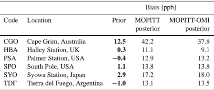
Table 4. Same as Table 3, but for the 6 stations chosen in the
high-latitudes of the Southern Hemisphere.
Biais [ppb]
Code Location Prior MOPITT MOPITT-OMI posterior posterior CGO Cape Grim, Australia 12.5 42.2 37.8 HBA Halley Station, UK 0.3 11.1 9.1 PSA Palmer Station, USA −0.4 12.9 13.2 SPO South Pole, USA 1.1 13.8 13.8 SYO Syowa Station, Japan 2.9 17.2 18.0 TDF Tierra del Fuego, Argentina −1.0 13.1 13.5
Ryori). We have computed the posterior and the prior bias be-tween the modeled and observed concentrations per station.
The inversion leads to a large improvement relative to the prior simulation for all the stations of Northern Hemisphere with an average reduction of the bias by about 60 %, except for the boreal station Ny-Alesund (increase of the bias by 10 %) due to the lack of satellites constraints in the high-latitudes. The largest improvement is seen for the station Sede Boker in Israel (WIS), where the inversion significantly decreases the emissions: the reduction of the bias reached about 80 % compared to the prior and to the “MOPITT-only” simulation. However, as seen in Table 4 and as already pointed out by Arellano et al. (2004) and by Stavrakou and
Southern Africa 18 19 17 17 18 19 18 19 18 19 18 19 Western Europe 35 29 35 29 35 29 35 38 35 28 35 31 Eastern Europe 31 28 31 29 31 31 31 31 31 30 31 30 Eurasian Boreal 28 24 29 30 28 31 29 29 29 28 29 28 Middle East 11 11 11 11 11 11 11 11 11 11 11 11 South Asia 63 72 63 73 63 76 63 76 63 69 63 72
South East Asia 84 95 84 95 86 95 84 90 84 91 84 96
Indonesia 35 34 34 36 32 38 32 36 32 37 32 34
Australia 11 10 11 10 11 10 11 9 11 9 11 11
Globe 491 515 490 518 491 552 486 537 486 520 486 523
M¨uller (2006), the fit is degraded at the high-latitude South-ern Hemisphere sites.
The mean global “MOPITT-OMI” posterior bias is es-timated at 11.6 ppb, 10 % smaller than the 12.8 ppb mean “MOPITT-only” posterior bias, confirming that the synergis-tic use of different datasets is required to better quantify CO emissions, even if the improvement is not clearly noticeable for some stations.
5.4.3 CH4surface emissions
Budget
The 6-yr average posterior CH4 emissions, from January
2005 to December 2010, presented in Table 5, are estimated at 529 TgCH4yr−1, higher by 8 % than the
correspond-ing prior (491 TgCH4yr−1). Our result is within the range
of 500–600 TgCH4 described in IPCC (2007). The main
changes between prior and posterior emissions are seen over USA (+18 %, from 50 to 61 TgCH4yr−1in 2005) and over
South Asia (+15 %, from 63 to 72 TgCH4yr−1in 2005). The
inversion highlights the importance of the South East Asia region as a CH4source with an average of 94 TgCH4yr−1,
followed by South Asia (74 TgCH4yr−1) and South
Ameri-can Temperate (53 TgCH4yr−1) regions.
6 Interannual variability
Global CH4emissions show significant IAV, with total flux
estimates ranging from 515 TgCH4(in 2005) to 552 TgCH4
(in 2007) (see Table 5). It could be noted that the 2008 global emissions are also high, with a total of 537 TgCH4yr−1.
The annual global budgets for 2009 and 2010 are estimated at, respectively, 520 TgCH4yr−1and 523 TgCH4yr−1. The
largest contributors to the global IAV of CH4emissions are
the tropical regions (South American Temperate, Northern Africa, South Asia, South East Asia and Indonesia). South American regions explain most of the observed atmospheric increase in 2007–2008.
Several studies attributed the IAV mostly to natural wet-lands (Dlugokencky et al., 2009; Bousquet et al., 2011). Fig-ure 9 shows the variation of the CH4 posterior emissions
and the CO posterior emissions, used as a proxy for biomass burning, over the temperate region South America. This re-veals that part of CH4flux IAV in this region can be related to
biomass burning emissions, at least in 2007. A peak of CH4
emissions appears to be correlated with a peak of CO emis-sions in September 2007, and to a lesser extent in September 2005, 2006 and 2008. It should be noted that 2007 was the year of the largest number of fires detected from space over the 2000–2009 period (Torres et al., 2010).
The mid-latitude and high-latitude CH4emissions (for the
regions USA, South American Tropical, Southern Africa, Middle East, Western and Eastern Europe, North American Boreal) seem to vary little from one year to the next (Ta-ble 5). However, the Eurasian Boreal annual budgets show that the 2007 CH4emissions are higher than in other years
(31 TgCH4yr−1, compared with 28 to 30 TgCH4yr−1 for
years 2005, 2006, 2008, 2009 and 2010). This can be related to higher temperatures complemented by changes in conti-nental precipitations impacting both methane flux densities and wetland extent in 2007 (Dlugokencky et al., 2009; Bous-quet et al., 2011).
Fig. 9. Seasonal cycles of the posterior CO and CH4 emissions for the tropical region South American Temperate, respectively in
TgCO/month and TgCH4/month, from January 2005 to December 2010.
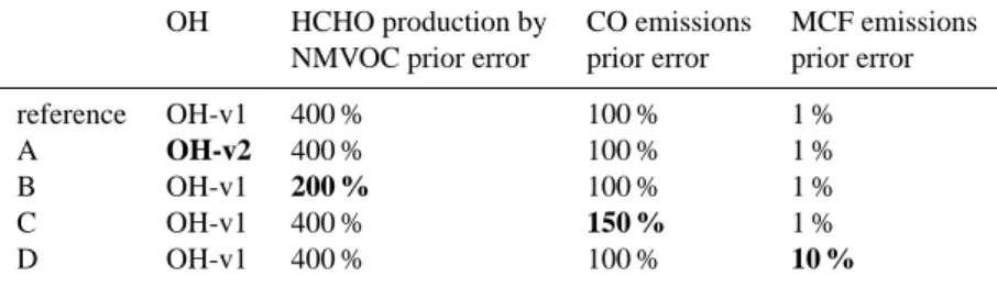
Table 6. Details of the sensitivity studies described in Sect. 6. The changes between the different sensitivity tests are highlighted in bold.
OH HCHO production by CO emissions MCF emissions
NMVOC prior error prior error prior error
reference OH-v1 400 % 100 % 1 % A OH-v2 400 % 100 % 1 % B OH-v1 200 % 100 % 1 % C OH-v1 400 % 150 % 1 % D OH-v1 400 % 100 % 10 % 7 Sensitivity studies
In this section, we discuss the robustness of our system from the spread of the regional HCHO production by NMVOC and of the regional CO and CH4emissions in four sensitivity
tests (cases A to D, described in Table 6) with respect to prior settings:
1. In case A, the OH field is replaced by OH-v2 field. The alternative field has also been derived from a simula-tion of the full chemistry model LMDz-INCA, but using another realistic emission scenario (the combination of anthropogenic emissions from IIASA, QUANTIFY for ship and GFEDv2 for biomass burning). OH-v2 field is within 5 % of the reference OH field. All other settings are the same as in the reference.
2. In case B, HCHO prior 3-D production by NMVOC er-ror is set to 200 % instead of 400 %.
3. In case C, CO prior emissions error is set to 150 % in-stead of 100 %.
4. In case D, MCF prior emissions error is set to 10 % in-stead of 1 %.
The HCHO production by NMVOC and CO and CH4
emis-sions for the whole year 2006, found from each test, are given for the 14 regions in Figs. 10a, 11a and 12a, re-spectively. These posterior regional results are further com-pared with the reference inversion in terms of anomalies in Figs. 10b, 11b and in Fig. 12b. For the three fields (HCHO production, CO and CH4 emissions). All sensitivity tests
present the same departure from the prior as the reference inversion. The different sensitivity tests show very robust re-gional and global budgets.
For CH4 (Fig. 12a), the differences in yearly methane
emission remain below 2 % at the global scale and range be-tween less than 1 % (Middle East, Southern Africa) to 12 % (Indonesia).
(a)
(b)
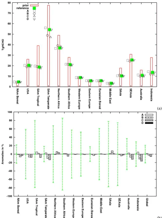
Fig. 10. (a) Regional 3-D HCHO production by NMVOC calculated for year 2006. The red bar represents the prior production and each
symbol a posterior production, for the reference inversion (in green) and the four sensitivity cases (in black). Case A: OH-v2 field; Case B: error on the HCHO 3-D production set to 200 %; Case C: error on the prior CO emissions set to 150 %; Case D: error on the prior MCF emissions set to 10 %. (b) Differences of the posterior HCHO production between the sensitivity tests and the reference inversion (in % relative to the reference). Error bars show the 1-σ uncertainty associated with the posterior reference (calculated using the Monte-Carlo approach, see Sect. 4 for details).
The regional estimates of 3-D HCHO production by NMVOC estimates obtained by the different sensitivity tests are also in a strong agreement. The largest range is observed over the regions Indonesia and South American Temperate (17 % and 15 %, respectively) because of the smaller incre-ments (compared to the reference) of cases B and C.
Nev-ertheless, these regional results are largely within the error bounds of the reference inversion (calculated with a robust Monte-Carlo approach, see Sect. 4).
The largest scatterings between the sensitivity tests are seen for CO emissions at the regional scale. While on the global scale, the sensitivity tests show results within 2 % of
(a)
(b)
Fig. 11. Same as Fig. 10, but for CO emissions.
the reference inversion, the differences reach up to 39 % at the regional scale. However, they are limited to 15 % in all re-gions emitting about or more than 100 TgCO yr−1(e.g. range of 14 TgCO over Southern Africa, for an annual reference budget of 133 TgCO), except for South East Asia (range of 51 TgCO for an annual reference budget of 208 TgCO).
The range of the inverted fluxes is well within the 1σ pos-terior uncertainty for all regions, except for the regions Mid-dle East, South East Asia and Indonesia. Finally, it is worth-noting that the difference between the regional inverted emis-sions in cases B, C and D relative to the reference inversion
is small, indicating that the inversion is not very sensitive to the prior errors statistics at the scales of interest here.
8 Conclusions
For the first time, an inversion of 3-D HCHO atmospheric production by NMVOC, carbon monoxide and methane emissions, together with OH concentrations, has been per-formed using a multi-constraint inversion system (using OMI and MOPITT satellite data, surface CH4and MCF
(a)
(b)
Fig. 12. Same as Fig. 10, but for CH4emissions.
concentrations with independent surface and aircraft mea-surements, and by computing sensitivity tests, we have demonstrated the robustness of our multi-species inversion system to assimilate a large number of data from different types (satellites, surface) over the period 2005–2010. We infer robust CO and CH4 emission and HCHO production
by NMVOC estimates. Such a robustness has been obtained despite the additional complexity implied by the connec-tion of three tracers and of OH within a single inversion system. Nevertheless, even though our approach allows to
widely spread adequate information between the tracers, it may probably spread biases as well.
Significant adjustments in the sources and sinks of formaldehyde are suggested in our study. The large reduc-tion of HCHO concentrareduc-tions, suggesting a large overestima-tion of the NMVOC emissions in the GEIA inventory, leads to a better agreement with the independent INTEX-B and AMMA data. The global posterior 3-D HCHO production by NMVOC of 257 TgHCHO is about 28 % smaller than the prior estimate of 358 TgHCHO.
The inversion leads to few changes in the OH concentra-tions from prior to posterior, and suggests a small interannual variability. The global mean posterior CH4emission flux of
529 TgCH4yr−1 is 8 % higher than the 490 TgCH4yr−1 of
the prior (on a 6-yr average). CH4emissions have some
sig-nificant interannual variability. The joint CO-CH4flux
anal-ysis suggests that tropical biomass burning probably played a role in the recent variations of atmospheric methane in South America. The highest annual budget over the period 2005– 2010 is calculated in 2007 with 552 TgCH4yr−1.
Our inverted global CO surface emission estimate is 1394 TgCO yr−1, 26 % higher than the corresponding prior but only 2 % smaller than the estimate of Fortems-Cheiney et al. (2011) who inverted CO emissions from MOPITT only as constraints. Significant regional changes appeared between the two studies, particularly for Middle East and South East Asia, improving the agreement between the posterior con-centrations and independent CO surface data in comparison to the single use of MOPITT. This highlights how promising the synergistic use of MOPITT, OMI and surface measure-ments for CH4and MCF is to avoid aliasing between
atmo-spheric chemistry (production and loss) signals and the fluxes at the surface and then to adjust the bottom-up inventories.
Our study relies on the quality of the HCHO column re-trievals. While OMI provides a daily coverage dataset at high spatial resolution, uncertainties remain large for OMI data, and the scarcity of in situ measurements remains an issue for evaluation and validation. More efforts should be devoted to the implementation of a common database with uncertainties or a global measurement network for HCHO – as it exists for greenhouse gases or other air pollutants such as CO – span-ning from urban to remote areas and from tropical to boreal regions.
Acknowledgements. This study was co-funded by the Euro-pean Commission under the EU Seventh Research Framework Programme (grant agreement No. 283576, MACC II). We ac-knowledge the KNMI OMI, the NCAR MOPITT, and the NOAA ESRL, Global Monitoring Division (GMD), Halocarbons & other Atmospheric Trace Species (HATS) and Carbon Cycle Greenhouse
Gases (CCGG) groups for providing HCHO, CO, MCF and CH4
measurements. We contacted all data PIs and in particular thank H. J. R. Wang (AGAGE), J. W. Elkins (NOAA), K. Masarie (NOAA), S. A. Montzka (NOAA), P. C. Novelli (NOAA), E. Dlu-gokencky (NOAA), P. Krummel (CSIRO), R. Langenfeld (CSIRO), P. Steele (CSIRO), D. Worthy (EC), R. Moss (NIWA), M. Ramonet (LSCE), and G. Brailsford (NIWA). This work was performed using HPC resources of DSM-CCRT and of (CCRT/CINES/IDRIS) under the allocation 2011-t2011012201 made by GENCI (Grand Equipement National de Calcul Intensif). Research at the Smithso-nian Astrophysical Observatory was supported by NASA. Finally, we wish to thank F. Marabelle and his team for computer support at LSCE.
Edited by: B. N. Duncan
The publication of this article is financed by CNRS-INSU.
References
Abbot, D. S., Palmer, P. I., Martin, R. V., Chance, K. V., Jacob, D. J., and Guenther, A.: Seasonal and interannual variability of North American isoprene emissions as determined by formalde-hyde columns measurements from space, Geophys. Res. Lett., 30, 1886, doi:10.1029/2003GL017336, 2003.
Arellano, A., Kasibhatla, P., Giglio, L., Van der Werf, G., and Randerson, J.: Top-down estimates of global CO using MOPITT measurements, Geophys. Res. Lett., 31, L01104, doi:10.1029/2003GL018609, 2004.
Barkley, M. P., Palmer, P. I., Kunh, U., Kesselmeier, J., Chance, K., Kurosu, T. P., Martin, R. V., Helmig, D., and Guenther, A.: Net ecosystem fluxes of isoprene over South America in-ferred from Global Ozone Monitoring Experiment (GOME) ob-servations of HCHO columns, Geophys. Res., 113, D20301, doi:10.1029/2008JD009863, 2008.
Bergamaschi, P., Frankenberg, C., Meirink, J. F., Krol, M., Vil-lani, M. G., Houweling, S., Den- tener, F., Dlugokencky, E. J., Miller, J. B., Gatti, L. V., Engel, A., and Levin, I.: Inverse
modeling of global and regional CH4 emissions using
SCIA-MACHY satellite retrievals, J. Geophys. Res., 114, D22301, doi:10.1029/2009JD012287, 2009.
Boeke, N. L., Marshall, J. D., Alvarez, S., Chance, K. V., Fried, A., Kurosu, T. P., Rappengluck, B., Richter, D., Walega, J., Weib-ring, P., and Millet, D. B.: Formaldehyde columns from the Ozone Monitoring Instrument: Urban versus background levels and evaluation using aircraft data and a global model, J. Geo-phys. Res., 116, D05303, doi:10.1029/2010JD014870, 2011. Borbon, A., Ruiz, M., Bechara, J., Aumont, B., Chong, M.,
Huntrieser, H., Mari, C., Reeves, C. E., Scialom, G., Ham-burger, T., Stark, H., Afif, C., Jambert, C., Mills, G., Schlager, H., and Perros, P. E.: Transport and chemistry of formaldehyde by mesoscale convective systems in West Africa during AMMA 2006, J. Geophys. Res., 117, D12301, doi:10.1029/2011JD017121, 2012.
Bousquet, P., Hauglustaine, D. A., Peylin, P., Carouge, C., and Ciais, P.: Two decades of OH variability as inferred by an in-version of atmospheric transport and chemistry of methyl chlo-roform, Atmos. Chem. Phys., 5, 2635–2656, doi:10.5194/acp-5-2635-2005, 2005.
Bousquet, P., Ciais, P., Miller, J., Dlugokencky, B., Hauglus-taine, D. A., Prigent, C., van der Werf, G. R., Peylin, P., Brunke, E.-G., Carouge, C., Langenfeld, R. L., Lathiere, J., Papa, F., Ramonet, M., Schmidt, M., Steele, L. P., Tyler, S. C., and White, J.: Contribution of anthropogenic and natural sources to atmospheric methane variability, Nature, 443, 439– 443, doi:10.1038/nature05132, 2006.
Bousquet, P., Ringeval, B., Pison, I., Dlugokencky, E. J., Brunke, E.-G., Carouge, C., Chevallier, F., Fortems-Cheiney, A.,
tions, J.Geophys. Res., 108, 8810, doi:10.1029/2002JD003116, 2003.
Chandra, S., Ziemke, J. R., Duncan, B. N., Diehl, T. L., Livesey, N. J., and Froidevaux, L.: Effects of the 2006 El Ni˜no on tro-pospheric ozone and carbon monoxide: implications for dynam-ics and biomass burning, Atmos. Chem. Phys., 9, 4239–4249, doi:10.5194/acp-9-4239-2009, 2009.
Chevallier, F., Fisher, M., Peylin, P., Serrar, S., Bousquet,
P., Breon, F.-M., Chedin, A., and Ciais, P.: Inferring CO2
sources and sinks from satellite observations: method and application to TOVS data, J. Geophys. Res., 110, D24309, doi:10.1029/2005JD006390, 2005.
Chevallier, F., Breon, F.-M., and Rayner, P.: The contribution of the Orbiting Carbon Observatory to the estimation of
CO2 sources and sinks: Theoretical study in a variational
data assimilation framework, J. Geophys. Res., 112, D09307, doi:10.1029/2006JD007375, 2007.
Chevallier, F., Fortems, A., Bousquet, P., Pison, I., Szopa, S., De-vaux, M., and Hauglustaine, D. A.: African CO emissions be-tween years 2000 and 2006 as estimated from MOPITT observa-tions, Biogeosciences, 6, 103–111, doi:10.5194/bg-6-103-2009, 2009.
Crawford, J., Heald, C., Fuelberg, H., Morse, D., Sachse, G., Em-mons, L., Gille, J., Edward, D., Deeter, M., Chen, G., Olson, J., Connors, V., Kittaka, C., and Hamlin, A.: Relationship between measurements of MOPITT and in-situ observations of CO based on a large-scale feature sampled during TRACE-P, J. Geophys. Res., 109, D15S04, doi:10.1029/2002JD004308, 2004. De Smedt, I., M¨uller, J.-F., Stavrakou, T., van der A, R., Eskes,
H., and Van Roozendael, M.: Twelve years of global obser-vations of formaldehyde in the troposphere using GOME and SCIAMACHY sensors, Atmos. Chem. Phys., 8, 4947–4963, doi:10.5194/acp-8-4947-2008, 2008.
Deeter, M., Edwards, D., Gille, J., Emmons, L., Francis, G., Ho, S.-P., Mao, D., Masters, D., Worden, H., Drummond, J., and Novelli, P.: The MOPITT Version 4 CO Product: Algorithm En-hancements, Validation, and Long-Term Stability, J. Geophys. Res., 115, D07306, doi:10.1029/2009JD013005, 2010.
Dentener, F., Peters, W., Krol, M., van Weele, M., Bergam-aschi, P., and Lelieveld, J.: Interannual variability and trend
of CH4 lifetime as a measure for OH changes in the
1979–1993 time period, J. Geophys. Res.-Atmos., 108, 4442, doi:10.1029/2002JD002916, 2003.
Dlugokencky, E. J., Bruhwiler, L., White, J. W. C, Emmons, L. K., Novelli, P. C., Montzka, S. A., Masarie, K. A., Lang, P. M., Crotwell, A. M., Miller, J. B., and Gatti, L. V.: Observational con-straints on recent increases in the atmospheric CH burden, Geo-phys. Res. Lett, 36, L18803, doi:10.1029/2009GL039780, 2009.
with aircraft in situ profiles, J. Geophys. Res., 108, D03309, doi:10.1029/2003JD004101, 2004.
Emmons, L., Pfister, G., Edwards, D., Gille, J., Sachse, G., Blake, D., Wofsy, S., Gerbig, C., ans Matross, D., and Nedelec, P.: MOPITT validation exercises during summer 2004 field cam-paigns over North America, J. Geophys. Res., 112, D12S02, doi:10.1029/2006JD007833, 2007.
Emmons, L. K., Edwards, D. P., Deeter, M. N., Gille, J. C., Cam-pos, T., N´ed´elec, P., Novelli, P., and Sachse, G.: Measurements of Pollution In The Troposphere (MOPITT) validation through 2006, Atmos. Chem. Phys., 9, 1795–1803, doi:10.5194/acp-9-1795-2009, 2009.
Folberth, G. A., Hauglustaine, D. A., Lathi`ere, J., and Brocheton, F.: Interactive chemistry in the Laboratoire de M´et´eorologie Dy-namique general circulation model: model description and im-pact analysis of biogenic hydrocarbons on tropospheric chem-istry, Atmos. Chem. Phys., 6, 2273–2319, doi:10.5194/acp-6-2273-2006, 2006.
Fortems-Cheiney, A., Chevallier, F., Pison, I., Bousquet, P., Szopa, S., Deeter, M. N., and Clerbaux, C.: Ten years of CO emissions as seen from Measurements of Pollution in the Troposphere (MOPITT), J. Geophys. Res., 116, D05304, doi:10.1029/2010JD014416, 2011.
Fried, A., Cantrell, C., Olson, J., Crawford, J. H., Weibring, P., Walega, J., Richter, D., Junkermann, W., Volkamer, R., Sinre-ich, R., Heikes, B. G., O’Sullivan, D., Blake, D. R., Blake, N., Meinardi, S., Apel, E., Weinheimer, A., Knapp, D., Perring, A., Cohen, R. C., Fuelberg, H., Shetter, R. E., Hall, S. R., Ullmann, K., Brune, W. H., Mao, J., Ren, X., Huey, L. G., Singh, H. B., Hair, J. W., Riemer, D., Diskin, G., and Sachse, G.: Detailed com-parisons of airborne formaldehyde measurements with box mod-els during the 2006 INTEX-B and MILAGRO campaigns: poten-tial evidence for significant impacts of unmeasured and multi-generation volatile organic carbon compounds, Atmos. Chem. Phys., 11, 11867–11894, doi:10.5194/acp-11-11867-2011, 2011. Fu, T.-M., Jacob, D. J., Palmer, P. I., Chance, K., Wang, Y. X., Barletta, B., Blake, D. R., Stanton, J. C., and Pilling, M. J.: Space-based formaldehyde measurements as constraints on volatile organic compound emissions in east and south Asia and implications for ozone, J. Geophys. Res., 112, D06312, doi:10.1029/2006JD007853, 2007.
Fung, I., John, J., Lerner, J., Matthew, E., Prather, M., Steele, P., and Fraser, P.: 3-Dimensional model synthesis of the global methane cycle, J. Geophys. Res., 96, 13033–13065, doi:10.1029/91JD01247, 1991.
Gilbert, J. and Lemar´echal, C.: Some numerical experiments with variable-storage quasi-Newton algorithms, Math. Programm, 45, 407–435, 1989.