HAL Id: hal-03125887
https://hal.archives-ouvertes.fr/hal-03125887
Preprint submitted on 29 Jan 2021
HAL is a multi-disciplinary open access
archive for the deposit and dissemination of
sci-entific research documents, whether they are
pub-lished or not. The documents may come from
teaching and research institutions in France or
abroad, or from public or private research centers.
L’archive ouverte pluridisciplinaire HAL, est
destinée au dépôt et à la diffusion de documents
scientifiques de niveau recherche, publiés ou non,
émanant des établissements d’enseignement et de
recherche français ou étrangers, des laboratoires
publics ou privés.
Multi-Tissue Multi-Compartment Models of Diffusion
MRI
Matteo Frigo, Rutger Fick, Mauro Zucchelli, Samuel Deslauriers-Gauthier,
Rachid Deriche
To cite this version:
Matteo Frigo, Rutger Fick, Mauro Zucchelli, Samuel Deslauriers-Gauthier, Rachid Deriche.
Multi-Tissue Multi-Compartment Models of Diffusion MRI. 2021. �hal-03125887�
Multi-Tissue Multi-Compartment Models of Diffusion MRI
Matteo Frigo
1,3, Rutger H.J. Fick
2, Mauro Zucchelli
1, Samuel Deslauriers-Gauthier
1, and
Rachid Deriche
11
Athena Project-Team, Inria Sophia Antipolis - Méditerranée, Université Côte D’Azur,
France
2
TRIBVN Healthcare, Paris, France
3Corresponding author: [email protected]
Abstract
State-of-the-art multi-compartment microstructural models of diffusion MRI (dMRI) in the human brain have limited capability to model multiple tissues at the same time. In particular, the available techniques that allow this multi-tissue modelling are based on multi-TE acquisitions. In this work we propose a novel multi-tissue formulation of classical multi-compartment models that relies on more common single-TE acquisitions and can be employed in the analysis of previously acquired datasets. We show how modelling multiple tissues provides a new interpretation of the concepts of signal fraction and volume fraction in the context of multi-compartment modelling. The software that allows to inspect single-TE diffusion MRI data with multi-tissue multi-compartment models is included in the publicly available Dmipy Python package.
Keywords diffusion MRI, microstructure, multi tissue, single-TE, volume fraction, signal fraction
1
Introduction
Diffusion MRI (dMRI) is an imaging technique that allows to inspect the brain tissue microstructure in-vivo non-invasively. One of the most commonly studied microstructural feature is the volume fraction of a tissue in a sample. In particular, the intra-axonal (i.e., intra-cellular - IC), extra-axonal (i.e., extra-cellular - EC) and cerebro-spinal fluid (CSF) volume fractions have been investigated with models like the neurite orientation dispersion and density imaging (NODDI) (Zhang et al.,2012), ActiveAx (Alexander et al.,2010), and the multi-compartment microscopic diffusion imaging framework (Kaden et al., 2016). The differences between these models lie on the representation employed in describing the tissue-specific signal and on the assumptions made on the model parameters. For example, intra-axonal diffusion can be modelled as the diffusion within a stick or a cylinder and some models fix the value of the diffusivity or tortuosity. A unifying aspect that characterizes most of the brain microstructure models is the building-blocks concept behind their formalisation. In other words, models are defined in a multi-compartment (MC) fashion, where the dMRI signal is described as a linear combination of single-tissue models. The resulting models are called MC models and they require the acquisition of multi-shell dMRI data in order to accurately disentangle the contribution of each compartment (Scherrer and Warfield,2010). Thorough reviews have been dedicated to the design and validation of such models (Jelescu and Budde, 2017), to the sensitivity of MC models to experimental factors and microstructural properties of the described tissues (Afzali et al.,2020), and to the abstraction of these models that allows to obtain a unified theory (Fick et al.,2019).
Recent studies have highlighted that all of the available MC models are transparent to the 𝑇2 relaxation times of the modelled tissues (Veraart et al.,2018;Lampinen et al.,2019). As a consequence, they implicitly assume that all the considered tissues have the same non-diffusion weighted signal 𝑆0. While this is a
reasonable assumption in some contexts, it is not true in general. In fact, each brain tissue is characterized by a specific relaxation time which makes 𝑇2 imaging possible. Assuming that all the tissues have a single
𝑆0 response simplify the model at the cost of biophysical accuracy. Tissue fractions obtained with this
assumption are called signal fractions, in contrast with the unbiased volume fractions which can be obtained with models that account for different 𝑆0responses of the modelled tissues. The former measures the linear
relation between the signal generated by a single tissue compartment and the acquired signal, while the latter measures the volume of single tissue compartment that is present in the voxel.
Given the known interdependence between the 𝑇2 times of tissues and the 𝑇 𝐸 of the acquisition, some attempts at addressing this issue have been formulated making use of multi-TE multi-shell dMRI acqui-sitions (Veraart et al., 2018; Lampinen et al., 2020; Gong et al., 2020). Despite allowing to increase the signal-to-noise ratio (SNR) (Eichner et al.,2020), these techniques require a complete re-design of the exper-iments from acquisition to post-processing, posing severe limitations in terms of usability of already acquired data. This aspect is crucial in modern neuroimaging, where large studies like the Human Connectome Project (HCP) (Van Essen et al., 2012), the UK Biobank (Sudlow et al., 2015) and the Alzheimer Disease Neuroimaging Initiative (ADNI) (Mueller et al.,2005) invest significant amounts of time and financial re-sources to acquire data of large cohorts with standardised protocols that need to be carefully designed a priori.
In this work1 we will show that the signal fractions are a biased estimation of the volume fractions and
that the latter can still be retrieved from the first without acquiring new data or re-fitting the MC model. We call this new technique, Multi-Tissue MC (MT-MC) model. To our knowledge MT-MC is the only model that estimates the volume fractions from single-TE multi-shell dMRI data. This novel formulation is inspired by the technique ofJeurissen et al.(2014) for the estimation of tissue-specific orientation distribution functions. The use of the MT-MC formulation solves some limitations of the previously mentioned multi-TE approaches and opens the door to the multi-tissue investigation of brain microstructure with data acquired with standard single-TE multi-shell dMRI protocols. Two algorithms for fitting the MT-MC model are proposed, one of which is designed to build on top of data already processed with standard MC models. Our new model is implemented and freely available in the Diffusion Microstructure Imaging in Python (Dmipy) (Fick et al.,
2019) framework, which is an open source tool designed for the abstraction, simulation, and fitting of MC models of dMRI. The ability of the MT-MC model to retrieve the unbiased volume fractions is tested on both synthetic data generated with Dmipy and real data obtained from the HCP database.
This article is organized as follows: Section 2 is devoted to the theoretical aspects of MC modelling, highlighting why signal and volume fractions are not equivalent in general, and to the formalization of the proposed MT-MC model. In Section3we will present the design of the experiments and in Section4we will show the corresponding results, which are then discussed in Section5, where also some conclusive remarks are presented.
2
Theory
2.1
Multi-Compartment models
Complex microstructural configurations can be modelled as a linear combination of few elementary com-partments. For example, the diffusion within axons can be described as the motion of water molecules along a stick or within a cylinder, while diffusion in free water, like the one that can be observed in the CSF, can be modelled as an isotropic 3D Gaussian function. A vast portion of the dMRI literature of the last twenty years is devoted to the definition of compartmental models for the anisotropic intra-axonal and extra-axonal diffusivity and for the isotropic diffusivity. These are known as Multi Compartment (MC) models and they all describe the shape of the normalized dMRI signal 𝐸 by means of the following linear combination of
1This work has partially been presented at the International Symposium on Biomedical Imaging of 2020 (Frigo et al.,2020a)
compartment-specific shapes: 𝐸(𝑏, 𝐆) = 𝑆(𝑏, 𝐆) 𝑆0 = 𝑁𝑐 ∑ 𝑖=1 𝜙𝑖⋅ 𝐸𝑖(𝑏, 𝐆) (1)
where 𝑏 is the 𝑏-value, 𝑆 is the raw diffusion signal, 𝑆0 is the diffusion signal acquired at 𝑏 = 0, and 𝐆 is the gradient direction, 𝑁𝑐 is the number of considered compartments, 𝐸𝑖 is the signal attenuation of compartment 𝑖, and 𝜙𝑖 is the portion of 𝐸 explained by compartment 𝑖, i.e. the signal fraction of the
compartment. The derivation of analytical expressions for the compartment-specific response functions has been researched broadly and deeply in the past literature. See the work ofPanagiotaki et al. (2014) for a thorough review of the topic. Among the most used MC models we can mention the stick-and-ball model ofBehrens et al.(2003), the ActiveAx model ofAlexander et al.(2010) and the neurite orientation dispersion and density imaging (NODDI) model of Zhang et al. (2012). A generalized MC model has been proposed byNovikov et al.(2019) in what they called the standard model of dMRI in the brain.
The standard model is composed of three compartments which, borrowing the taxonomy fromPanagiotaki et al.(2014), are defined as follows:
• The IC compartment is modelled as a stick whose free parameters are the parallel diffusivity 𝜆∥ and
the direction of the fiber population as the unit vector 𝐧. The corresponding signal is given by 𝐸𝐼𝐶(𝑏, 𝐆, 𝜆∥, 𝐧) = 𝑒−𝑏𝜆∥⟨𝐧,𝐆⟩ (2)
where ⟨𝐧, 𝐆⟩ denotes the usual scalar product in ℝ2.
• The EC component is described by an axially symmetric Gaussian function (i.e., zeppelin), which can be defined as a diffusion tensor that depends on the parallel diffusivity 𝜆∥, the perpendicular diffusivity
𝜆⟂and the direction of the fiber population 𝐧 (which is assumed to be the same as the one of the stick compartment). The signal shape is given by the classical tensor model
𝐸𝐸𝐶(𝑏, 𝐆, 𝜆∥, 𝜆⟂, 𝐧) = 𝑒−𝑏𝐆
𝑇𝐷𝐆
(3) where the diffusion tensor is defined as 𝐷 = (𝜆∥− 𝜆⟂) 𝐧𝐧𝑇+ 𝜆⟂𝐼 and 𝐼 is the 3-by-3 identity matrix.
• The CSF compartment is modelled an isotropic Gaussian function (i.e., ball), which is defined as a zeppelin with 𝜆∥= 𝜆⟂= 𝜆𝑟where 𝜆𝑟is the radial diffusivity. The expression for the signal shape reads as follows:
𝐸𝐶𝑆𝐹(𝑏, 𝜆𝑟) = 𝑒−𝑏𝜆𝑟. (4)
Notice that the first term in the definition of the diffusion tensor disappears, hence the model does not depend on the principal direction 𝐧, making the compartment isotropic as wanted.
Additionally, fiber dispersion is formalized as the convolution of the stick and zeppelin compartments with an ODF denoted by 𝒫. An example of such orientation function is the Watson distribution 𝑊 (𝐧, 𝜅) (Mardia and Jupp,1990), which assumes axial symmetry of the dispersion around the main direction of the bundle 𝐧 ∈ 𝕊2 with concentration 𝜅. The corresponding orientation dispersion index (ODI) can be computed as
𝑂𝐷𝐼 = 2/𝜋 ⋅ arctan(1/𝜅) (Zhang et al.,2012).
Given the elements described in the previous lines, the MC formulation of the standard model is defined as
𝐸(𝐧, 𝜅, 𝜆∥, 𝜆⟂, 𝜆𝑟, 𝜙𝐼𝐶, 𝜙𝐸𝐶, 𝜙𝐶𝑆𝐹) =
𝒫(𝐧) ∗ [𝜙𝐼𝐶 ⋅ 𝐸𝐼𝐶(𝜆∥, 𝐧) + 𝜙𝐸𝐶⋅ 𝐸𝐸𝐶(𝜆∥, 𝜆⟂, 𝐧)] + 𝜙𝐶𝑆𝐹 ⋅ 𝐸𝐶𝑆𝐹(𝜆𝑟) (5) where ∗ is spherical convolution operator and the dependence on the acquisition parameters 𝑏 and 𝐆 has been omitted for the sake of readability. Several constraints can be applied to the model given in Equation (5), among which the most commons are:
• the sum of the signal fractions is unitary: 𝜙𝐼𝐶+ 𝜙𝐸𝐶+ 𝜙𝐶𝑆𝐹 = 1;
• the perpendicular diffusivity of the EC compartment is tortuous (Szafer et al., 1995a,b), which in mathematical terms means
𝜆⟂=
𝜙𝐸𝐶
𝜙𝐼𝐶+ 𝜙𝐸𝐶
⋅ 𝜆∥; (6)
• the parallel diffusivity of the IC and EC compartments is fixed (e.g. 𝜆∥= 1.7 ⋅ 10−9𝑚2/𝑠 as in (Zhang et al.,2012));
• the radial diffusivity of the CSF compartment is fixed (e.g. 𝜆𝑟 = 3.0 ⋅ 10−9𝑚2/𝑠 as in (Zhang et al., 2012)).
Recent studies questioned the validity of these constraints (Jelescu et al., 2016; Lampinen et al., 2017;
Dell’Acqua and Tournier,2019).
As highlighted by the left hand side of Equation (5), the model depends on eight parameters, where 𝐧 is two-dimensional, yielding 9 degrees of freedom, to which one has to subtract the degrees of freedom covered by the constraints. The remaining parameters can be estimated solving the minimization problem
𝑝∗= argmin 𝑝 1 2∥ ̂ 𝑆 ̂ 𝑆0 − 𝐸(𝑝)∥ 2 2 (7)
where 𝑝 is the parameter vector,𝑆 is the acquired dMRI signal,̂ 𝑆0̂ is the mean 𝑏 = 0 image and 𝐸(𝑝) is the realization of the forward model given in Equation (5). Fitting such parameters requires the acquisition of multi-shell data with at least one shell per compartment (Scherrer and Warfield,2010). The obtained pa-rameters 𝑝∗are the microstructural parameters that can finally be analysed for clinical or research purposes.
In practice, the fitted signal fractions 𝜙𝑖 will likely not sum to 1, as they absorb any discrepancies between
the normalised signal in the left hand side and the signal shapes in the left hand sides of Equation (5), in particular when more than one image is acquired at 𝑏 = 0.
A thorough review on the variety of MC models of WM that can be defined with the current state-of-the-art tools is the one ofFick et al.(2019), where also the Dmipy package is presented. This software is the reference tool used throughout this work for the study of microstructure. More recently, MC models have been used to assess also the microstructural composition of the gray matter (GM) (Ganepola et al.,
2018;Fukutomi et al.,2019;Villalon-reina et al.,2020), but the literature is still sparse and there is a lack of agreement on how to model the GM with MC models.
The key operation behind the definition of MC models is the division of the diffusion-weighted signal 𝑆 by the non-diffusion-weighted component 𝑆0, which allows to retrieve the signal shape which is then modelled as the linear combination of the signal shape of the compartments that characterize the model. In the next section we are going to question the applicability of this division by 𝑆0.
2.2
MC models do not account for T2 differences
As stated in the previous section and formalised in Equation (1), MC models aim at fitting the signal attenuation 𝐸 as the ratio of the PGSE signal 𝑆 and the 𝑆0 amplitude. The implicit assumption that
lies behind this formulation is that the 𝑆0 by which the acquired signal is divided is the same for all the modelled compartments. In particular, as the 𝑆0 image corresponds to the signal coming from the non-diffusion-weighted spin-echo sequence, we know that its amplitude depends on the echo time 𝑇 𝐸 and the repetition time 𝑇 𝑅 of the acquisition and on the 𝑇1 and 𝑇2 times of the sample. The relationship between these quantities reads as
𝑆0∼ [𝐻] ⋅ (1 − 𝑒−𝑇 𝑅/𝑇1) ⋅ 𝑒−𝑇 𝐸/𝑇2 (8)
where [𝐻] is the proton density in the sample. While in the formation of the 𝑆0image the different 𝑇1times
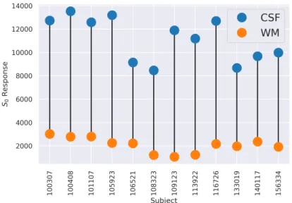
Figure 1: The figure shows the 𝑆0response of the WM and of the CSF for twelve randomly picked subjects
from the HCP database. Values are obtained with the heuristic technique of Dhollander et al. (2016) via Mrtrix3 (Tournier et al.,2019).
𝑇 𝐸), tissues with different 𝑇2 will generate sensibly different contrast in the image (Plewes,1994;Just and Thelen,1988;Veraart et al.,2018). Figure1illustrates how this difference is visible in the 𝑆0response of the
WM and the CSF. These differences are the result of the different contrast in 𝑇2-weighted images between
the different compartments. In order to understand how this difference in the 𝑇2 impacts the signal-fraction
estimation, consider the following example. Let a voxel in the WM containing some partial volume of CSF, which is common in the corpus-callosum near the ventricles. In particular, let’s assume that the volume fractions are 𝑓𝑊 𝑀 = 0.9 and 𝑓𝐶𝑆𝐹 = 0.1. The corresponding signal equation will be
𝑆 = 0.9 ⋅ 𝑆𝑊 𝑀
0 ⋅ 𝐸𝑊 𝑀+ 0.1 ⋅ 𝑆0𝐶𝑆𝐹 ⋅ 𝐸𝐶𝑆𝐹. (9)
As highlighted by Figure1, the value of 𝑆𝐶𝑆𝐹
0 can be up to six times the one of 𝑆0𝑊 𝑀. Including this into
our toy model, hence defining 𝑆𝐶𝑆𝐹
0 = 6 ⋅ 𝑆0𝑊 𝑀, Equation (9) becomes
𝑆 = 0.9 ⋅ 𝑆𝑊 𝑀
0 ⋅ 𝐸𝑊 𝑀+ 0.6 ⋅ 𝑆0𝑊 𝑀⋅ 𝐸𝐶𝑆𝐹 (10)
which after dividing both sides of the equation by the composite 𝑆0= 𝑓𝑊 𝑀⋅ 𝑆0𝑊 𝑀+ 𝑓𝐶𝑆𝐹⋅ 𝑆𝐶𝑆𝐹0 becomes
𝑆 𝑆0
= 0.6 ⋅ 𝐸𝑊 𝑀+ 0.4 ⋅ 𝐸𝐶𝑆𝐹 (11)
yielding the signal fractions 𝜙𝑊 𝑀 = 0.6 and 𝜙𝐶𝑆𝐹 = 0.4. This exampled showed how signal fractions
and volume fractions are not interchangeable concepts when it comes to modelling multiple tissues having different 𝑆0 responses. Not taking into account this differences can lead to significant misrepresentations of
the tissue composition, as showed in the previous example and in the results reported in Section4.
2.3
Leveraging multi-TE sequences in Multi-Compartment modelling of the
dMRI signal
If the problem of MC models is that they do not distinguish the 𝑆0 of different tissues because of the limitations of single-TE acquisition sequences like the one considered in the previous sections, the solution could simply be to use multi-TE (MTE) acquisitions, despite the required longer acquisition time. This
idea has been investigated in recent works ofVeraart et al.(2018),Lampinen et al.(2019,2020), and Gong et al.(2020). These works are all based on the assumptions that the volume fraction of a tissue can not be computed with conventional multi-shell dMRI data acquired with a single echo time.
The TE-dependent Diffusion Imaging (TEdDI) technique proposed by Veraart et al. (2018) technique considers a rewriting of the MC equation that directly includes the contribution of the 𝑇2time of the tissue
modelled by the compartment and the 𝑇 𝐸 of the acquisition into the volume fraction of each compartment. The same principles are followed in the more recent works ofLampinen et al.(2019,2020) and ofGong et al.
(2020). For the sake of coherence, we adapted the original notation used in the articles. The TEdDI model is designed to account for the 𝑇 𝐸/𝑇2 effects in the same way as in the 𝑆0-image formation process described in Equation (8), obtaining 𝑆(𝑏, 𝑇 𝐸, 𝑇𝑖 2, 𝐩𝑖) = 𝑆0⋅ 𝑁𝑐 ∑ 𝑖=1 𝜙𝑖⋅ 𝑒−𝑇 𝐸/𝑇𝑖 2 ⋅ 𝐸 𝑖(𝑏, 𝐩𝑖), 𝑁𝑐 ∑ 𝑖=1 𝜙𝑖= 1 (12) where 𝑒−𝑇 𝐸/𝑇𝑖
2 plays the role of the compartment-specific contribution of the 𝑇
2 time. Notice that the
𝑇2 time of each compartment is an independent variable of the model, hence it must be estimated in the
fitting process. This requires the acquisition of multi-shell (to allow the use of multiple compartments) and multi-TE (to avoid degeneracy in the joint fitting of 𝜙𝑖 and 𝑇2𝑖) dMRI data. The volume fraction of each
compartment is defined byVeraart et al.(2018) andGong et al.(2020) as follows:
𝑓𝑖(𝑇 𝐸) = 𝜙𝑖⋅ 𝑒 −𝑇 𝐸/𝑇𝑖 2 ∑𝑗𝜙𝑗⋅ 𝑒−𝑇 𝐸/𝑇𝑗 2 (13)
where one should notice how the volume fraction 𝑓𝑖 depends on the echo time 𝑇 𝐸. Conversely,Lampinen et al.(2019,2020) opted for defining the volume fractions as
𝑓𝑖=
𝜙𝑖
∑𝑗𝜙𝑗
, (14)
which corresponds to the normalisation of the 𝜙𝑖 retrieved from fitting the model given in Equation (12).
The formulation provided in Equation (12) can be regarded as the multi-TE standard model of the dMRI signal in the human brain, in analogy with what reported byNovikov et al.(2019) (see Equation (5)).
The MTE standard model has already been used in the previously cited works ofVeraart et al.(2018), Lam-pinen et al. (2019, 2020) and Gong et al. (2020) to investigate the microstructure of the white matter of the brain. They showed that particular instances of the MTE standard model allow to assess how the 𝑇2 time of the acquired sample is formed by the different compartments. Also, with MTE-MC models they showed that the concept of volume fraction should not just be abandoned in favor of the concept of signal
fraction. Its straightforward interpretability is of much appeal in brain pathology research (Suzuki et al.,
2017;Hara et al.,2018;Vestergaard-Poulsen et al.,2007), where biomarkers are not only quantified but also contextualized, related to other non-microstructural information and interpreted.
Some limitations come with the use of such formulation. First, the volume fractions defined in Equa-tion (13) are 𝑇 𝐸-dependent. This poses severe limitations in terms of usability and prevents from having a single index for the volume fraction of a compartment, which intuitively should be a characteristic of the sample, not of the acquisition. This ambiguity adds itself to the second limitation of the MTE formulation, which concerns how the 𝑇2 time of the tissue modelled by each compartment is included in the model. As
shown in Equation (12), the MTE framework corrects the classical MC model by multiplying each term in the sum by the 𝑇2-dependent factor Equation (8) of the 𝑆0 image, which is exactly 𝑒−𝑇 𝐸/𝑇2. This
contri-bution to the signal 𝑆 is counted twice, as it is implicitly present also in the 𝑆0 term that multiplies the
sum on the right hand side of Equation (12). Notice that relaxing the ∑𝑁𝑐
𝑖=1𝜙𝑖 = 1 constraint would solve
the issue, as the double contribution would be corrected by an identical scaling of each 𝜙𝑖, which is then
the term affects the fitting of the 𝑇2times is out of the scope of this work. The third limitation of MTE-MC
modelling that we highlight is of methodological nature. Classical MC models are representations of the dMRI signal that rely on standard multi-shell acquisitions designed in a HARDI fashion which have been used in the last 15 years for the study of both microstructure and tractography-based structural connectiv-ity. The MTE framework does have the merit to correct the signal/volume fraction ambiguity, but this is achieved by increasing the complexity of the acquisition, which requires multiple 𝑇 𝐸 to be considered. For this reason, the MTE framework is not to be considered an alternative to the MC formulation but rather a new method for the estimation of microstructural parameters that spans the whole range from acquisition design to post-processing, preventing from correcting the estimation of volume fractions on datasets acquired in the past.
2.4
Multi-Tissue Multi-Compartment models
The standard formulation of MC models includes a normalization of the dMRI signal 𝑆0by its
non-diffusion-weighted component 𝑆0. This operation is performed in order to retrieve the shape 𝐸 of the acquired signal. The shape is then modelled as a linear combination of signal shapes of different compartments. In Section2.2
we showed how this formulation hides the assumption that all the tissues modelled by the compartments have the same 𝑇2time (hence 𝑆0), highlighting how this is not true a-priori. The solutions to the multi-tissue problem proposed in the literature have the remarkable limitation of requiring the acquisition of multi-TE data to be used.
A solution to a similar problem has been proposed by Jeurissen et al. (2014) in the context of fODF estimation for multi-shell data, where the shell- and tissue-specific signal amplitude is leveraged in order to rescale the fODF that describes the signal shape of each considered tissue. This includes the response of each tissue in the 𝑏 = 0 shell, hence the 𝑆0 of the tissues. The technique we are proposing builds on top of
this idea.
Let 𝑁𝑐 be the number of compartments included in the model we want to design and let 𝑆0𝑖 be the 𝑆0
response of compartment 𝑖. We define the Multi-Tissue Multi-Compartment (MT-MC) model as follows:
𝑆 (𝑏, 𝑇 𝐸) = 𝑁𝑐 ∑ 𝑖=1 𝑓𝑖⋅ 𝑆𝑖 0(𝑇 𝐸) ⋅ 𝐸𝑖(𝑏, p𝑖) (15)
where 𝑓𝑖 is the volume fraction of compartment 𝑖 and 𝑆0𝑖(𝑇 𝐸) is the 𝑆0 response of the tissue modelled by
compartment 𝑖. Notice that Equation (15) is equivalent to Equation (1) whenever 𝑆𝑖 0 = 𝑆
𝑗
0 ∀ 𝑖, 𝑗, namely
when all the tissues described by the MT-MC model have equal 𝑆0 responses.
In general, the signal fraction 𝜙𝑖 is not equivalent to the volume fraction 𝑓𝑖 of the tissue modelled by
the compartment. The only case in which they are equivalent is when all the tissues modelled by the MT-MC model have equal 𝑆0 responses. In that case, Equation (15) reduces to (1) after multiplying both
the sides by 𝑆0. For this reason we say that 𝜙𝑖 is a biased estimator of 𝑓𝑖. One could argue that the
relationship between the signal fractions 𝜙𝑖 and the volume fractions 𝑓𝑖 is just a rescaling, in which case the volume fractions could be retrieved with a simple correction that takes into account the 𝑆0 signal and the 𝑆𝑖
0 response of the compartment. This is true, except when the volume fraction of the compartment is an
independent variable in some other compartment, as for the case of the tortuosity constraint. In that case, the perpendicular diffusivity of the extra-axonal compartment is a function of the volume fraction of the intra-axonal compartment. This makes the intra-axonal volume fraction a non-linear independent parameter of the model, therefore it can not be transformed into the corresponding signal fraction (or vice-versa) with the aforementioned rescaling.
2.4.1 Fitting MT-MC models
The fitting of a MT-MC model is designed in a fashion similar to the one of MC models. Here we propose two different approaches. The first is a direct fitting that provides only the volume fractions (VF), while the second is a two-step strategy that builds on top of the fitting of the signal fractions and yields both the signal
and the volume fractions (SVF), allowing to re-process in a MT fashion results that had previously been obtained on standard MC models. Given the acquired dMRI signal 𝑆, the corresponding 𝑆0, the number of
compartments 𝑁𝑐, the signal shape 𝐸𝑖(𝐩𝑖) of compartment 𝑖 depending on the parameter vector 𝐩𝑖and the
compartment-specific signal amplitude 𝑆𝑖
0, the fitting can be performed in the two following ways.
VF The first approach directly fits the volume fractions by solving a least squares problem with respect to the microstructural parameters 𝑓𝑖 and 𝐩𝑖:
𝑓∗, 𝑝∗= argmin 𝑓𝑖,𝑝𝑖 ∥𝑆 − 𝑁𝑐 ∑ 𝑖=1 𝑓𝑖⋅ 𝑆0𝑖⋅ 𝐸𝑖(𝐩𝑖)∥ 2 2 (16)
which can be solved with ordinary inverse-problem solvers. Here, the forward model is the one given in Equation (15). The procedure yields the volume fractions (VF) of the compartments.
SVF The second approach extracts the volume fractions after fitting the signal fractions 𝜙𝑖 and the
mi-crostructural parameters 𝐩𝑖 from the MC formulation of Equation (5). The volume fractions are retrieved
as a rescaling of the signal fractions. The described procedure reads as follows: 1. Solve the associated MC problem:
𝜙∗, 𝐩∗= argmin 𝜙𝑖,𝐩𝑖 ∥𝑆 𝑆0 − 𝑁𝑐 ∑ 𝑖=1 𝜙𝑖⋅ 𝐸𝑖(𝐩𝑖)∥ 2 2 (17)
where the product of the minimization problem is the signal fraction 𝜙𝑖 and the parameter vector 𝐩𝑖 of each compartment 𝑖;
2. Fix the fitted non-signal-fraction parameters in the MT-MC model. At this point the volume fractions are not related to each other (or to other compartments in general) and it is therefore possible to estimate them by rescaling the signal fractions. The rescaling is the one suggested by the comparison of the coefficients that multiply the signal shapes in Equations (1) and (15) and reads as follows:
𝑓𝑖⋅ 𝑆0𝑖 = 𝜙𝑖⋅ 𝑆0 𝑓𝑖= 𝜙𝑖⋅ 𝑆0 𝑆𝑖 0 (18)
yielding a simple operation that allows to retrieve volume fractions from signal fractions once the 𝑆0of
each compartment is known. Both the signal and volume fractions of each compartment are returned. To employ either of the two fitting strategies, extra caution must be taken towards the use of the tortuosity constraint. The intra- and extra- axonal fractions used for the definition of the perpendicular diffusivity can be either the signal fractions or the volume fractions of the compartments, i.e.,
𝜆⟂= 𝜙𝐸𝐶 𝜙𝐼𝐶+ 𝜙𝐸𝐶 𝜆∥ or 𝜆⟂= 𝑓𝐸𝐶 𝑓𝐼𝐶+ 𝑓𝐸𝐶 𝜆∥. (19)
The choice influences the whole model design and can not be reverted in the fitting process. In particular, switching between signal fractions and volume fractions with the 𝑆0/𝑆0𝑖 rescaling must be done keeping in
mind that the tortuous parameters have been obtained using a specific type of fraction, and the results should be interpreted accordingly. In an effort to keep the notation coherent with the previous literature, we will say that whenever the tortuosity constraint is defined using the volume fractions 𝑓𝑖 we will have a
MT-corrected tortuosity constraint.
The SVF strategy is the one implemented in Dmipy (Fick et al., 2019), which to our knowledge is the only available framework for MC modelling that includes the definition of MT-MC models.
2.5
The MT Standard Model of dMRI in White Matter
In this Section, we define a MT generalization of the standard model of dMRI in WM as described byNovikov et al.(2019). We recall that the model includes a stick and a zeppelin compartment for the intra- and extra-cellular diffusivity respectively and a ball that accounts for the isotropic diffusivity in the CSF. Let 𝑆𝑖
0 be
the 𝑆0 response of the tissue modelled by each compartment 𝑖 and 𝒫 ∶ 𝕊2→ ℝ+the orientation distribution.
The MT standard model of dMRI in WM is given by
𝑆(𝐧, 𝜅, 𝜆∥, 𝜆⟂, 𝜆𝑟, 𝑓𝐼𝐶, 𝑓𝐸𝐶, 𝑓𝐶𝑆𝐹) = 𝑃 (𝐧) ∗ ⎛⎜⎜ ⎝ 𝑓𝐼𝐶⋅ 𝑆𝐼𝐶 0 ⋅ 𝐸𝐼𝐶(𝜆∥, 𝐧) ⏟⏟⏟⏟⏟⏟⏟⏟⏟ intra-axonal + 𝑓𝐸𝐶⋅ 𝑆𝐸𝐶 0 ⋅ 𝐸𝐸𝐶(𝜆∥, 𝜆⟂, 𝐧) ⏟⏟⏟⏟⏟⏟⏟⏟⏟⏟⏟⏟⏟ extra-axonal ⎞ ⎟ ⎟ ⎠ + 𝑓⏟⏟⏟⏟⏟⏟⏟⏟⏟⏟⏟𝐶𝑆𝐹 ⋅ 𝑆𝐶𝑆𝐹0 ⋅ 𝐸𝐶𝑆𝐹(𝜆𝑟) 𝐶𝑆𝐹 (20)
where the compartment specific parameters are defined as in Section2.1. Three scenarios can be described with this model:
• 3-tissue model - The three compartments describe tissues with distinct 𝑆0responses. This corresponds
to the explicit case of Equation (20).
• 2-tissue model - The two anisotropic compartments model tissues whose 𝑆0 is equal. Typically, it is the 𝑆0 of the WM, so we say that 𝑆𝐼𝐶
0 = 𝑆0𝐸𝐶= 𝑆0𝑊 𝑀 and 𝑆0𝑊 𝑀≠ 𝑆0𝐶𝑆𝐹.
• 1-tissue model - In absence of any prior knowledge on the 𝑆0 of the three tissues, they are considered
all equal. We denote this as 𝑆𝐼𝐶
0 = 𝑆0𝐸𝐶 = 𝑆0𝐶𝑆𝐹 = 𝑆0 where 𝑆0 is the average across the images
acquired at 𝑏 = 0 𝑠/𝑚𝑚2.
Notice that the 1-tissue scenario is mathematically equivalent to the single-tissue (ST) standard model of Equation (20), hence in that case the volume fractions are equivalent to the signal fractions.
3
Methods
3.1
Dataset
3.1.1 Synthetic data
The simulated dataset is obtained from the forward model given by Equation (20) and generated with Dmipy (Fick et al.,2019). A total of 10000 voxels was simulated on a multi-shell acquisition scheme identical to the one that will be considered on the real dataset, which includes a TE of 0.0895𝑠 and is composed of 288 samples subdivided in 18 points at 𝑏 = 0𝑠/𝑚𝑚2 and 90 diffusion-weighted samples obtained with
uniformly distributed directions at 𝑏 = 1000𝑠/𝑚𝑚2, 𝑏 = 2000𝑠/𝑚𝑚2 and 𝑏 = 3000𝑠/𝑚𝑚2 for a total of 3
diffusion-weighted shells plus the 𝑏 = 0 shell. The direction of the two anisotropic compartments was set to 𝐧 = [0, 0] ∈ 𝕊2 for all the voxels. The 𝑇
2 time of each tissue was randomly sampled from a uniform
distribution in the range specified in Table1. The corresponding 𝑆0was then computed as 𝑆0= 𝑐 ⋅ 𝑒−𝑇 𝐸/𝑇2
where 𝑐 is a scaling parameter that positions the value of 𝑆0in a realistic range and we tuned to 𝑐 = 1400. The
ODI of the Watson distribution was sampled from a uniform distribution in the range specified in Table1. Finally, the volume fractions of each compartment were randomly generated from a uniform distribution in the range specified in Table1, then normalized in such a way that their sum was equal to 1. The choice of each range was tuned to mimic the single-bundle configuration in the WM that one expects to be able to model with the considered formulation. An additive rician noise was added to the simulated data to obtain a signal-to-noise ratio equal to 30.
Parameter Min Max 𝑓𝐼𝐶 0.5 0.8 𝑓𝐸𝐶 0.3 0.5 𝑓𝐶𝑆𝐹 0.3 0.7 𝑇𝐼𝐶 2 0.080𝑠 0.100𝑠 𝑇𝐸𝐶 2 0.050𝑠 0.070𝑠 𝑇𝐶𝑆𝐹 2 0.900𝑠 1.100𝑠 𝑂𝐷𝐼 0.02 0.99
Table 1: For each parameter used in the definition of the forward model of the synthetic dataset we report the minimum and maximum value of the uniform distribution from which it was drawn.
3.1.2 Real data
From the Human Connectome Project (HCP) database we considered three randomly picked subjects2
available at the Connectome Coordination Facility (Van Essen et al., 2012; Sotiropoulos et al., 2013). For each subject a total of 288 images is acquired, subdivided in 18 volumes at 𝑏 = 0𝑠/𝑚𝑚2 and 90
diffusion-weighted volumes obtained at uniformly distributed directions at 𝑏 = 1000𝑠/𝑚𝑚2, 𝑏 = 2000𝑠/𝑚𝑚2 and
𝑏 = 3000𝑠/𝑚𝑚2 for a total of 3 shells. All subjects provided written informed consent, procedures were
approved by the ethics committee and the research was performed in compliance with the Code of Ethics of the World Medical Association (Declaration of Helsinki).
To our knowledge, current state-of-the-art techniques do not allow to estimate subject-specific 𝑆0 re-sponses of the IC and EC compartments, while the 𝑆0 of the CSF compartment can be estimated together with 𝑆𝑊 𝑀
0 via techniques such as the heuristic approach of Dhollander et al. (2016). For this reason, we
analysed the aforementioned data with a 1-tissue and a 2-tissue model where 𝑆𝑊 𝑀
0 and 𝑆0𝐶𝑆𝐹 have been
estimated with the Dhollander technique. The obtained values of 𝑆0are displayed in Figure1 and reported
in Table2. Subject 𝑆𝑊 𝑀 0 𝑆0𝐶𝑆𝐹 #1 3024 12740 #2 2794 13531 #3 2811 12598
Table 2: 𝑆0 response of the WM and of the CSF of the three studied HCP subjects. Values are obtained with the heuristic technique ofDhollander et al.(2016) via Mrtrix3 (Tournier et al.,2019).
3.2
Model fitting
The model considered in the performed experiments is the MT standard model defined in the previous section with fixed 𝑆𝑖
0 and three additional constraints:
• The fiber orientation distribution is modelled with a Watson distribution of axis 𝐧 and fixed ODI. • The perpendicular diffusivity is subject to the tortuosity constraint, hence
𝜆⟂= (1 −
𝑓𝐼𝐶
𝑓𝐼𝐶+ 𝑓𝐸𝐶
) ⋅ 𝜆∥. (21)
• The parallel and radial diffusivity are fixed to 𝜆∥= 1.7⋅10−9𝑚2𝑠−1and 𝜆𝑟= 3.0⋅10−9𝑚2𝑠−1respectively.
The free parameters that are left are [𝑓𝐼𝐶, 𝑓𝐸𝐶, 𝑓𝐼𝑆𝑂, 𝐧, 𝜅], where we recall that the unit vector 𝐧 is expressed
in spherical coordinates [𝜃, 𝜑]. The fitting was performed with Dmipy (Fick et al.,2019, version 1.0.3) using the SVF procedure described in Section2.4.1 in order to retrieve both the signal fractions and the volume fractions to be compared.
4
Results
4.1
Synthetic data
We fitted the volume fractions𝑓𝑖̂ of each compartment with the SVF procedure explained in Section2.4.1
with the 1-tissue, 2-tissue and 3-tissue model, both with standard and MT-corrected tortuosity. The latter is actually different from the standard tortuosity only when the 3-tissue model is considered. When the 2-tissue model is employed, the 𝑆𝑊 𝑀
0 response is computed as the weighted average of the 𝑆0 response of
the IC and EC compartments, hence
𝑆𝑊 𝑀 0 =
𝑓𝐼𝐶⋅ 𝑆0𝐼𝐶+ 𝑓𝐸𝐶⋅ 𝑆0𝐸𝐶
𝑓𝐼𝐶+ 𝑓𝐸𝐶
. (22)
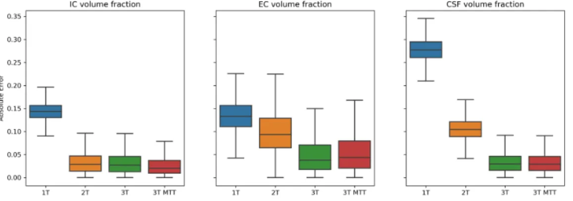
Once each 𝑓𝑖̂ was estimated, we computed the absolute fitting error ∣𝑓𝑖− ̂𝑓𝑖∣. In Figure 2 we report the
boxplot of the distribution of the absolute fitting error across all the simulations. As we expected, the signal
Figure 2: Boxplot of the absolute error of the estimated volume fraction of each compartment computed on the synthetic dataset. The 1T categorical variable corresponds to the 1-tissue model, 2T to the 2-tissue, 3T to the 3-tissue with standard tortuosity and 3T MTT to the 3-tissue model with MT-corrected Tortuosity (MTT).
fractions retrieved by the 1-tissue model are biased estimates of the volume fractions retrieved with the 2-tissue and 3-tissue model. The bias in the estimation of the volume fraction of the CSF compartment is four times bigger than the one of the IC and EC compartment. This is coherent with the fact that the 𝑆0
of the CSF compartment is much higher than the one of the IC and EC compartments. The error decreases importantly when the 2-tissue model is used. Here, the IC volume fraction has absolute error comparable to the one of the 3-tissue models. The first factor that could induce such phenomenon is the definition of 𝑆𝑊 𝑀
0 , which by design of the experiment will be closer to the 𝑆0 of the IC than to the one of the EC
compartment (𝑓𝐼𝐶 > 𝑓𝐸𝐶 as reported in Table 1). This induces the estimated EC volume fraction to be farther from the ground truth than the one of the IC compartment. This difference is reflected in the absolute error of the estimated volume fraction of the CSF compartment, which is affected by the presence of the non-zero perpendicular diffusivity of the EC compartment. Nevertheless, the estimation error of the CSF volume fraction is much lower than in the 1-tissue model thanks to the inclusion of the specific 𝑆𝐶𝑆𝐹
formulation. Finally, the 3-tissue model retrieves volume fractions that are in line with the ground truth ones. We highlight how the inclusion of the MT-correction of the tortuosity constraint does not sensibly benefit the fitting. We hypothesise that the effects of the inclusion of the MT-correction are lower than the ones made by the noise included in the system.
4.2
Real data
For each model, we fitted the signal and volume fractions with the SVF technique. Figure 3 shows the distribution of the signal fraction and volume fraction of each compartment in the WM for three HCP subjects. The WM mask was computed with FSL fast from the 𝑇1-weighted image with 1.25𝑚𝑚 voxel size
available at the HCP database, then dilated by one voxel with Mrtrix3’s (Tournier et al., 2019) maskfilter command to smooth the boundary.
Figure 3: The displayed data are obtained three subjects of the HCP database (solid lines, dashed lines, and dotted lines). Each panel shows the distribution of the signal fraction and the volume fraction of the IC, EC and CSF compartments respectively. The blue lines correspond to signal fractions and the orange lines to
volume fractions.
We recall that we considered a 2-tissue model by compressing the IC and EC compartments in a unique block that describes the WM tissue. The distribution of the volume fractions of the IC and EC compartments showed in Figure3is right-shifted with respect to the distribution of the corresponding signal fractions. On the contrary, the distribution of CSF volume fractions in the WM mask is shifted towards lower values with respect to the corresponding signal fractions. This means that the signal fraction underestimates the presence of the intracellular compartment in favour of the CSF compartment. This behaviour is consisted in all the tested subjects and the three distributions are consistent between the subjects for all the tissues. This is coherent with the proportion between 𝑆𝑊 𝑀
0 and 𝑆0𝐶𝑆𝐹, as the former is typically lower than the
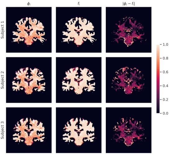
acquired 𝑆0 and the latter is higher. The results displayed in Figure4show how, within the WM mask, the WM volume fraction is globally higher than the WM signal fraction. Also, the absolute difference between the two exhibits some uniformity within the considered sample. The macroscopic differences between the left and right hemispheres present in all the three subjects may be due to some bias field effect that we did not include in the model and survived the minimal preprocessing of the data (Glasser et al.,2013).
Figure 4: Signal fractions (first column), volume fractions (second column), and their absolute difference (third column) for three subjects of the HCP database. Brighter colors correspond to higher fractions (in the first two columns) and errors (in the third column). Voxels shown in orange/red and black correspond to decreasingly lower values of the same fractions and errors.
5
Discussion and Conclusions
In this paper we analysed how multi-compartment models of brain tissue microstructure can be adapted to account for the presence of tissues having different 𝑇2 relaxation times. In particular, we focused on the
capability of such models to estimate the volume fraction of each tissue in the WM. We proposed a solution based on single-TE dMRI data, in contrast with the state-of-the-art techniques that require multi-TE dMRI data. Our results on both synthetic and in-vivo data show that signal fraction and volume fraction are not interchangeable concepts in the context of MC microstructure modelling. The shift of paradigm from signal fractions to volume fractions has already been shown to improve the estimation of fODFs (Jeurissen et al., 2014) and in this work we transferred the same approach to the field of MC models of brain tissue microstructure, leveraging the differences between the 𝑆0 responses of each modelled tissue.
Overall, the presented results yielded an empirical confirm of the theoretical considerations made in this work. In particular, the following aspects are highlighted:
• With single-TE dMRI data it is possible to retrieve tissue-specific volume fractions. Under the assump-tion that the IC and EC compartments have equal 𝑆0 response, techniques like the one ofDhollander et al. (2016) allow to define the 2-tissue model used in this section, opening the door to a better estimation of the compartment-specific volume fractions. This is made possible by the MT-version of
the standard model of dMRI in the WM that we presented in this work. It models multiple tissues in a MC fashion without requiring multi-TE acquisition, which are conversely necessary in order to use other state-of-the-art models.
• Signal fractions and volume fractions are not equivalent in general. This fact has considerable im-plications in clinical context. Previous studies that drew conclusions based on the idea of inspecting volume fractions with single-TE dMRI need to be re-interpreted in light of the fact that what they are based on is the signal fraction of the tissues and not their volume fraction. How those differences are expressed in the presence of pathology or group differences remains unexplored and needs to be assessed in future studies.
We designed a multi-tissue version of the standard model of dMRI in the WM, which allows to separate the contribution of the intra-axonal, the extra-axonal and the CSF compartments and estimate the corresponding three volume fractions. The results reported in Figure2suggest that 2-tissue and 3-tissue models are always preferable to the 1-tissue model. A bigger improvement is obtained by considering two tissues instead of one, compared to the shift from the 2-tissue to the 3-tissue model. This is due to the proportion between the 𝑆0s of each tissue, which sees 𝑆0𝐶𝑆𝐹 >> 𝑆0𝑊 𝑀, with 𝑆0𝐼𝐶 > 𝑆0𝐸𝐶 but the latter difference is lower than
the former (Jeurissen et al.,2014).
A remarkable property of the proposed MT-MC model is that not only it can be straightforwardly fitted on single-TE dMRI data (VF strategy), but it can also re-use the results obtained with the MC version of the model (which in principle would have returned only the signal fraction of each compartment) and yield the volume fractions by means of an elementary rescaling operation (SVF strategy). While employing the SVF solution, extra care must be devoted to the use of the tortuosity constraint. Rescaling signal fractions obtained using the non-MT-corrected tortuosity constraint yields the volume fractions of a model where some diffusivity has been obtained using signal fractions, configuring an ambiguous (if not degenerate) solution. Nevertheless, the extent of the effect of including the MT-correction of tortuosity does not justify its inclusion. It remains unclear whether the effect of the correction is absorbed by the noise of the data or by the mixed contribution of the zeppelin and the ball compartment. Further studies are necessary to address this issue.
The proposed model strongly relies on the external estimation of the 𝑇2or the 𝑆0of the modelled tissues.
Our experiments on real data leveraged the heuristic ofDhollander et al.(2016) to retrieve the 𝑆0of the WM
and the CSF. Understanding how this choice affects the estimation of volume fractions is out of the scope of this work, but the raised question suggests that further efforts should be devoted to researching techniques that estimate tissue-specific 𝑆0 responses using single-TE data. Additionally, analysing the proportion between the 𝑆0of each tissue in a large cohort of subjects could highlight patterns that could be exploited. If hypothetically the 𝑇2 of extra-axonal was showed to be a constant fraction of the 𝑇2 of the intra-axonal compartment, this could straightforwardly be encoded in the model.
The difference between signal fractions and volume fractions has implications also in the field of tractog-raphy filtering, where a coefficient is assigned to each streamline in a tractogram weighing its contribution to the formation of the dMRI signal. In the COMMIT framework (Daducci et al.,2015) these coefficients are the signal fractions associated to each streamline. The model can be easily adapted to obtain the volume fraction associated to each streamline, in particular in the context of the recent work of Barakovic et al.
(2020), where streamlines are associated to bundle-specific 𝑇2 times.
In this work, we analyzed the brain tissue microstructure estimation via multi-compartment models of dMRI. We tackled the known limitation concerning the inability of state-of-the-art multi-compartment models to describe multiple tissues having distinct 𝑇2 relaxation times. We showed how what has always
been considered the volume fraction of a certain tissue is actually the signal fraction of the same tissue. State-of-the-art techniques for overtaking such limitation rely on multi-TE dMRI data. Here, we introduced the Multi-Tissue Multi-Compartment models of dMRI, which allow to model multiple tissues at the same time using single-TE dMRI data. Moreover, we formulated a generalised multi-tissue modelling framework that encompasses both TE and multi-TE multi-tissue models. Our results indicate that with single-TE dMRI data alone one can model multiple tissues at the same time using the proposed multi-tissue multi-compartment models.
Acknowledgements
This work was funded by the European Research Council (ERC) under the European Union’s Horizon 2020 research and innovation program (ERC Advanced Grant agreement No 694665: CoBCoM - Computational Brain Connectivity Mapping). Data were provided by the Human Connectome Project, WU-Minn Consor-tium (Principal Investigators: David Van Essen and Kamil Ugurbil; 1U54MH091657) funded by the 16 NIH Institutes and Centers that support the NIH Blueprint for Neuroscience Research; and by the McDonnell Center for Systems Neuroscience at Washington University. This work has been supported by the French government, through the 3IA Côte D’Azur Investments in the Future project managed by the National Research Agency (ANR) with the reference number ANR-19-P3IA-0002.
Declaration of competing interest
The authors declare that they have no known competing financial interests or personal relationships that could have appeared to influence the work reported in this paper.
Open science
In this work we used only publicly available data from the Human Connectome Project database (Van Essen et al.,2012) and open source code from the Dmipy (Fick et al.,2019, version 1.0.3) Python package and the Mrtrix3 (Tournier et al.,2019) suite.
References
M. Afzali, T. Pieciak, S. Newman, E. Garifallidis, E. Özarslan, H. Cheng, and D. K. Jones. The sensitivity of diffusion mri to microstructural properties and experimental factors. Journal of Neuroscience Methods, page 108951, 2020.
D. C. Alexander, P. L. Hubbard, M. G. Hall, E. A. Moore, M. Ptito, G. J. Parker, and T. B. Dyrby. Orientationally invariant indices of axon diameter and density from diffusion mri. Neuroimage, 52(4): 1374–1389, 2010.
M. Barakovic, C. M. Tax, U. S. Rudrapatna, M. Chamberland, J. Rafael-Patino, C. Granziera, J.-P. Thiran, A. Daducci, E. J. Canales-Rodríguez, and D. K. Jones. Resolving bundle-specific intra-axonal t2 values within a voxel using diffusion-relaxation tract-based estimation. NeuroImage, page 117617, 2020.
T. E. Behrens, M. W. Woolrich, M. Jenkinson, H. Johansen-Berg, R. G. Nunes, et al. Characterization and propagation of uncertainty in diffusion-weighted mr imaging. Magnetic Resonance in Medicine: An
Official Journal of the International Society for Magnetic Resonance in Medicine, 50(5):1077–1088, 2003.
A. Daducci, A. Dal Palù, A. Lemkaddem, and J.-P. Thiran. Commit: convex optimization modeling for microstructure informed tractography. IEEE transactions on medical imaging, 34(1):246–257, 2015. F. Dell’Acqua and J.-D. Tournier. Modelling white matter with spherical deconvolution: How and why?
NMR in Biomedicine, 32(4):e3945, 2019.
T. Dhollander, D. Raffelt, and A. Connelly. Unsupervised 3-tissue response function estimation from single-shell or multi-single-shell diffusion mr data without a co-registered t1 image. In ISMRM Workshop on Breaking
the Barriers of Diffusion MRI, volume 5, page 2016, 2016.
C. Eichner, M. Paquette, T. Mildner, T. Schlumm, K. Pléh, L. Samuni, C. Crockford, R. M. Wittig, C. Jäger, H. E. Möller, et al. Increased sensitivity and signal-to-noise ratio in diffusion-weighted mri using multi-echo acquisitions. Neuroimage, 2020.
R. Fick, D. Wassermann, and R. Deriche. The dmipy toolbox: Diffusion mri multi-compartment modeling and microstructure recovery made easy. Frontiers in Neuroinformatics, 13(64), 2019. doi: /10.3389/ fninf2019.00064.
M. Frigo, R. Fick, M. Zucchelli, S. Deslauriers-Gauthier, and R. Deriche. Multi tissue modelling of diffusion mri signal reveals volume fraction bias. In 2020 IEEE 17th International Symposium on Biomedical
Imaging (ISBI), pages 991–994. IEEE, 2020a.
M. Frigo, M. Zucchelli, R. Fick, S. Deslauriers-Gauthier, and R. Deriche. Multi-compartment modelling of diffusion mri signal shows te-based volume fraction bias. In OHBM 2020-26th meeting of the Organization
of Human Brain Mapping, pages hal–02925963, 2020b.
H. Fukutomi, M. F. Glasser, K. Murata, T. Akasaka, K. Fujimoto, T. Yamamoto, J. A. Autio, T. Okada, K. Togashi, H. Zhang, et al. Diffusion tensor model links to neurite orientation dispersion and density imaging at high b-value in cerebral cortical gray matter. Scientific reports, 9(1):1–12, 2019.
T. Ganepola, Z. Nagy, A. Ghosh, T. Papadopoulo, D. C. Alexander, and M. I. Sereno. Using diffusion mri to discriminate areas of cortical grey matter. NeuroImage, 182:456–468, 2018.
M. F. Glasser, S. N. Sotiropoulos, J. A. Wilson, T. S. Coalson, B. Fischl, et al. The minimal preprocessing pipelines for the human connectome project. Neuroimage, 80:105–124, 2013.
T. Gong, Q. Tong, H. He, Y. Sun, J. Zhong, and H. Zhang. Mte-noddi: Multi-te noddi for disentangling non-t2-weighted signal fractions from compartment-specific t2 relaxation times. NeuroImage, page 116906, 2020.
S. Hara, M. Hori, S. Murata, R. Ueda, Y. Tanaka, M. Inaji, T. Maehara, S. Aoki, and T. Nariai. Microstruc-tural damage in normal-appearing brain parenchyma and neurocognitive dysfunction in adult moyamoya disease. Stroke, 49(10):2504–2507, 2018.
I. O. Jelescu and M. D. Budde. Design and validation of diffusion mri models of white matter. Frontiers in
physics, 5:61, 2017.
I. O. Jelescu, J. Veraart, E. Fieremans, and D. S. Novikov. Degeneracy in model parameter estimation for multi-compartmental diffusion in neuronal tissue. NMR in Biomedicine, 29(1):33–47, 2016.
B. Jeurissen, J.-D. Tournier, T. Dhollander, A. Connelly, and J. Sijbers. Multi-tissue constrained spherical deconvolution for improved analysis of multi-shell diffusion mri data. NeuroImage, 103:411–426, 2014. M. Just and M. Thelen. Tissue characterization with t1, t2, and proton density values: results in 160 patients
with brain tumors. Radiology, 169(3):779–785, 1988.
E. Kaden, N. D. Kelm, R. P. Carson, M. D. Does, and D. C. Alexander. Multi-compartment microscopic diffusion imaging. NeuroImage, 139:346–359, 2016.
B. Lampinen, F. Szczepankiewicz, J. Mårtensson, D. van Westen, P. C. Sundgren, and M. Nilsson. Neurite density imaging versus imaging of microscopic anisotropy in diffusion mri: A model comparison using spherical tensor encoding. Neuroimage, 147:517–531, 2017.
B. Lampinen, F. Szczepankiewicz, M. Novén, D. van Westen, O. Hansson, E. Englund, J. Mårtensson, C.-F. Westin, and M. Nilsson. Searching for the neurite density with diffusion mri: challenges for biophysical modeling. Human brain mapping, 40(8):2529–2545, 2019.
B. Lampinen, F. Szczepankiewicz, J. Mårtensson, D. van Westen, O. Hansson, C.-F. Westin, and M. Nilsson. Towards unconstrained compartment modeling in white matter using diffusion-relaxation mri with tensor-valued diffusion encoding. Magnetic Resonance in Medicine, 84(3):1605–1623, 2020.
K. V. Mardia and P. E. Jupp. Directional statistics, volume 494. John Wiley & Sons, 1990.
S. G. Mueller, M. W. Weiner, L. J. Thal, R. C. Petersen, C. Jack, W. Jagust, J. Q. Trojanowski, A. W. Toga, and L. Beckett. The alzheimer’s disease neuroimaging initiative. Neuroimaging Clinics, 15(4):869–877, 2005.
D. S. Novikov, E. Fieremans, S. N. Jespersen, and V. G. Kiselev. Quantifying brain microstructure with diffusion mri: Theory and parameter estimation. NMR in Biomedicine, 32(4):e3998, 2019.
E. Panagiotaki, S. Walker-Samuel, B. Siow, S. P. Johnson, V. Rajkumar, R. B. Pedley, M. F. Lythgoe, and D. C. Alexander. Noninvasive quantification of solid tumor microstructure using verdict mri. Cancer
research, 74(7):1902–1912, 2014.
D. B. Plewes. Contrast mechanisms in spin-echo mr imaging. Radiographics, 14(6):1389–1404, 1994. B. Scherrer and S. K. Warfield. Why multiple b-values are required for multi-tensor models. evaluation with
a constrained log-euclidean model. In 2010 IEEE International Symposium on Biomedical Imaging: From
Nano to Macro, pages 1389–1392. IEEE, 2010.
S. N. Sotiropoulos, S. Jbabdi, J. Xu, J. L. Andersson, S. Moeller, E. J. Auerbach, M. F. Glasser, M. Her-nandez, G. Sapiro, M. Jenkinson, et al. Advances in diffusion mri acquisition and processing in the human connectome project. Neuroimage, 80:125–143, 2013.
C. Sudlow, J. Gallacher, N. Allen, V. Beral, P. Burton, J. Danesh, P. Downey, P. Elliott, J. Green, M. Lan-dray, et al. Uk biobank: an open access resource for identifying the causes of a wide range of complex diseases of middle and old age. Plos med, 12(3):e1001779, 2015.
H. Suzuki, H. Gao, W. Bai, E. Evangelou, B. Glocker, D. P. O’Regan, P. Elliott, and P. M. Matthews. Abnormal brain white matter microstructure is associated with both pre-hypertension and hypertension.
PLoS One, 12(11):e0187600, 2017.
A. Szafer, J. Zhong, A. W. Anderson, and J. C. Gore. Diffusion-weighted imaging in tissues: theoretical models. NMR in Biomedicine, 8(7):289–296, 1995a. ISSN 10991492. doi: 10.1002/nbm.1940080704. A. Szafer, J. Zhong, and J. C. Gore. Theoretical model for water diffusion in tissues. Magnetic resonance in
medicine, 33(5):697–712, 1995b.
J.-D. Tournier, R. Smith, D. Raffelt, R. Tabbara, T. Dhollander, M. Pietsch, D. Christiaens, B. Jeurissen, C.-H. Yeh, and A. Connelly. Mrtrix3: A fast, flexible and open software framework for medical image processing and visualisation. NeuroImage, 202:116137, 2019.
D. C. Van Essen, K. Ugurbil, E. Auerbach, D. Barch, T. Behrens, R. Bucholz, A. Chang, L. Chen, M. Cor-betta, S. W. Curtiss, et al. The human connectome project: a data acquisition perspective. Neuroimage, 62(4):2222–2231, 2012.
J. Veraart, D. S. Novikov, and E. Fieremans. Te dependent diffusion imaging (teddi) distinguishes between compartmental t2 relaxation times. NeuroImage, 182:360–369, 2018. ISSN 1053-8119. doi: 10.1016/j.neuroimage.2017.09.030. URL http://www.sciencedirect.com/science/article/pii/ S1053811917307784.
P. Vestergaard-Poulsen, B. Hansen, L. Østergaard, and R. Jakobsen. Microstructural changes in ischemic cortical gray matter predicted by a model of diffusion-weighted mri. Journal of Magnetic Resonance
Imaging: An Official Journal of the International Society for Magnetic Resonance in Medicine, 26(3):
529–540, 2007.
J. E. Villalon-reina, T. M. Nir, S. I. Thomopoulos, L. E. Salminen, R. Fick, M. Frigo, R. Deriche, P. M. Thompson, and ADNI. Tracking microstructural biomarkers of Alzheimer’s disease via advanced multi-shell diffusion MRI scalar measures. In ISMRM, page 2020, 2020.
H. Zhang, T. Schneider, C. A. Wheeler-Kingshott, and D. C. Alexander. Noddi: practical in vivo neurite orientation dispersion and density imaging of the human brain. Neuroimage, 61(4):1000–1016, 2012.