Behavioral Equivalences for Higher-Order Languages with Probabilities

(1)

HAL Id: tel-01644462

https://hal.inria.fr/tel-01644462

Submitted on 22 Nov 2017

HAL is a multi-disciplinary open access archive for the deposit and dissemination of sci-entific research documents, whether they are pub-lished or not. The documents may come from teaching and research institutions in France or abroad, or from public or private research centers.

L’archive ouverte pluridisciplinaire HAL, est destinée au dépôt et à la diffusion de documents scientifiques de niveau recherche, publiés ou non, émanant des établissements d’enseignement et de recherche français ou étrangers, des laboratoires publics ou privés.

with Probabilities

Valeria Vignudelli

To cite this version:

Valeria Vignudelli. Behavioral Equivalences for Higher-Order Languages with Probabilities. Logic in Computer Science [cs.LO]. University of Bologna, 2017. English. �tel-01644462�

(2)

Alma Mater Studiorum – Universit`

a di Bologna

DOTTORATO DI RICERCA IN

COMPUTER SCIENCE AND ENGINEERING Ciclo XXIX

Settore Concorsuale di afferenza: 01/B1 Settore Scientifico Disciplinare: INF/01

Behavioral Equivalences for Higher-Order

Languages with Probabilities

Presentata da: Valeria Vignudelli

Coordinatore Dottorato Paolo Ciaccia

Relatore Davide Sangiorgi

(3)

(4)

Abstract

Higher-order languages, whose paradigmatic example is the λ-calculus, are languages with powerful operators that are capable of manipulating and exchanging programs themselves. This thesis studies behavioral equivalences for programs with higher-order and probabilis-tic features. Behavioral equivalence is formalized as a contextual, or testing, equivalence, and two main lines of research are pursued in the thesis.

The first part of the thesis focuses on contextual equivalence as a way of investigating the expressiveness of different languages. The discriminating powers offered by higher-order concurrent languages (Higher-Order π-calculi) are compared with those offered by higher-order sequential languages (`a la λ-calculus) and by first-order concurrent languages (`a la CCS). The comparison is carried out by examining the contextual equivalences in-duced by the languages on two classes of first-order processes, namely nondeterministic and probabilistic processes. As a result, the spectrum of the discriminating powers of several varieties of higher-order and first-order languages is obtained, both in a nondeterministic and in a probabilistic setting.

The second part of the thesis is devoted to proof techniques for contextual equivalence in probabilistic λ-calculi. Bisimulation-based proof techniques are studied, with particular focus on deriving bisimulations that are fully abstract for contextual equivalence (i.e., coincide with it). As a first result, full abstraction of applicative bisimilarity and similarity are proved for a call-by-value probabilistic λ-calculus with a parallel disjunction operator. Applicative bisimulations are however known not to scale to richer languages. Hence, more robust notions of bisimulations for probabilistic calculi are considered, in the form of environmental bisimulations. Environmental bisimulations are defined for pure call-by-name and call-by-value probabilistic λ-calculi, and for a (call-by-value) probabilistic λ-calculus extended with references (i.e., a store). In each case, full abstraction results are derived.

(5)

(6)

Acknowledgments

I am deeply grateful to my advisor, Davide Sangiorgi, for constantly supporting me and for giving me great opportunities to learn and to grow as a researcher. He has always been available to patiently answer my questions, to suggest enlightening solutions, and to share and discuss new ideas. I owe him a lot for all the time he devoted to me.

I want to express my gratitude to Christel Baier and Eijiro Sumii, for accepting to review this thesis and for providing insightful comments and suggestions.

In the past three years, I had the pleasure to work with many inspiring people, whom I thank. In Bologna, I had enriching discussions and collaborations with Ugo Dal Lago, Marco Bernardo, and Rapha¨elle Crubill´e. In Paris, I had the chance to work with Catuscia Palamidessi and Kostas Chatzikokolakis, and to learn about exciting new topics.

The work in this thesis is also the result of the opportunities I had to discuss it in different venues. In particular, I am grateful to Lars Birkedal, Luke Ong, and Damien Pous for inviting me to present my work.

I greatly profited from discussions with people in the Focus team, and with past and present colleagues. Thank you all. I especially want to thank Francesco Gavazzo, Jean-Marie Madiot, and Saverio Giallorenzo, who have been helpful friends and PhD fellows.

(7)

(8)

List of Figures

2.1 Spectrum for LTSs . . . 26

2.2 Strictness of inclusions in the spectrum for RPLTSs . . . 29

2.3 Operational semantics for pure λ-calculi . . . 32

3.1 Syntax of Λloc . . . 36

3.2 Reduction rules of Λloc(L) for L an LTS . . . 37

3.3 Reduction rules of Λloc(L) for L an RPLTS . . . 41

3.4 Syntax for HOπpass,ref . . . 44

3.5 Operational semantics for HOπpass,ref(L) . . . 44

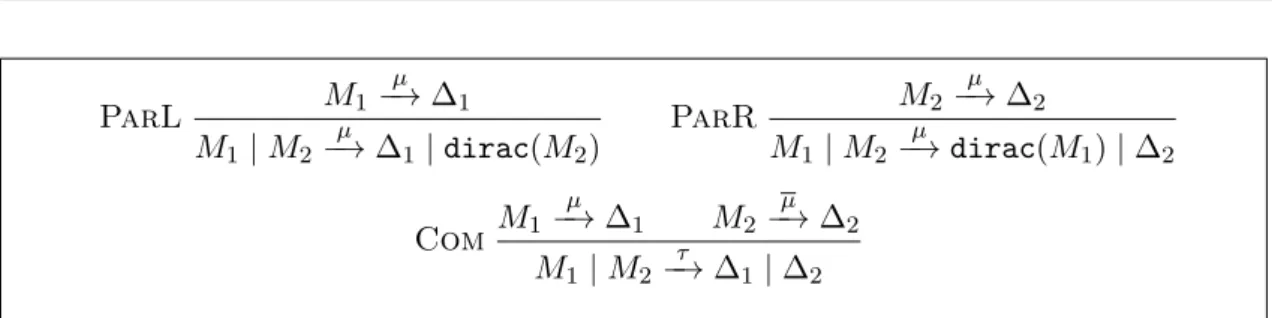
3.6 Rules for parallel composition in the probabilistic setting . . . 45

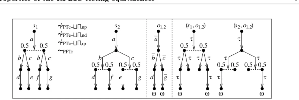
4.1 Counterexample for testing equivalences and probabilistic failure trace equiv-alence on RPLTSs . . . 71

4.2 Counterexamples for probabilistic bisimilarity and testing equivalences on RPLTSs . . . 72

4.3 Deprobabilization of an RRPLTS test (applies recursively to T1, T2, . . . , Tn) 73 5.1 The spectrum of equivalences for nondeterministic processes . . . 82

5.2 The spectrum of equivalences for reactive probabilistic processes . . . 83

6.1 Single-step reduction relation for imperative λ-calculus . . . 92

6.2 Operational semantics for pure probabilistic λ-calculi . . . 94

7.1 RPLTS for M, N . . . 99

7.2 Big-step semantics for parallel disjunction . . . 100

7.3 Howe’s construction . . . 103

8.1 Operational semantics for call-by-name . . . 118

8.2 Formal sums as matrices . . . 129

8.3 Single-step reduction relation for imperative probabilistic λ-calculus . . . . 138

(13)

(14)

Chapter 1

Introduction

Program equivalence is a delicate notion. Nevertheless, there is a unifying and general way of defining what it means for two systems to be equivalent with respect to their behavior. This is given by the so-called contextual, or testing, equivalences: contexts of some language play the role of tests, and two programs or systems are contextually equivalent if the execution of the same test returns the same observation. More formally, given two systems S1 and S2(the tested systems), a language L that we can use to interact with the systems (the testing language), and an observation Obs (the result of the tests), we say that S1 and S2 are contextually equivalent in L if whenever we put them in the same context C of L we have Obs(C[S1]) = Obs(C[S2]). This definition of contextual equivalence thereby formalizes the idea of behavioral equivalence as interchangeability, or indistiguishability, in a black-box testing scenario.

The study of contextually-defined equivalences has been pursued along different paths: • analyzing the discriminating power of a language, as compared to other languages. In this case, we are studying the expressiveness of a language by looking at the kind of tests a context of the language can perform;

• studying methods allowing us to prove that two programs in a language are con-textually equivalent (with respect to the same language). This approach is thereby devoted to finding proof techniques for contextual equivalence.

The first perspective has been adopted in particular in concurrency theory, in which several varieties of testing scenarios have been proposed. Given a class C of tested systems, we look at how one or more languages interact with systems in C. Then language L1 is strictly more discriminating than language L2 if whenever S1 and S2 are equivalent with respect to tests (or contexts) in L1 then they are also equivalent with respect to tests in L2, and there are systems that can be discriminated by L1 but are equal in L2.

In the second line of research, we typically consider contextual equivalences where both the tested programs and the contexts are from the same language L. Contextual equivalence defines what it means for two programs in the language to be equivalent, and we look for efficient methods to prove program equivalence.

In both cases, however, the characterization of contextually-defined equivalences in terms of equivalences whose definition is not directly of the form “for all contexts of the lan-guage...” or “for all tests...” plays a crucial role. When studying the expressiveness of a language, we aim at characterizing the contextual equivalence it induces on some class C

(15)

of systems as an equivalence that is directly defined on the systems and does not mention the testing language. This gives us a way of comparing the testing equivalences induced by different languages with each other. On the other side, if we are interested in proving contextual equivalence for a language, we can see that the universal quantification over all contexts of a language makes it hard to exhibit proofs of equivalence. This holds in particular for higher-order languages, whose operators are capable of manipulating and exchanging programs themselves. In this setting, bisimulation-based equivalences have been shown to provide efficient proof methods for contextual equivalences.

This thesis analyzes program equivalence for higher-order languages along these two main lines of research: expressiveness and proof techniques. In particular, we focus on how higher-order languages interact with probabilistic systems and features.

The theory of functional higher-order languages, starting from λ-calculi, has been thor-oughly studied in the literature, and higher-order languages for concurrent and distributed systems have been investigated as well. The interest in probabilistic programming and computation has been growing for the last few years, motivated, for instance, by the need of modeling complex systems evolving with some degree of uncertainty, and by the need of implementing randomized algorithms for both efficiency and security reasons. Proba-bilistic languages, equivalences, and models have been thereby proposed to this end, and they now form an established and productive research topic.

In the presence of probabilities, the definition of program equivalence must take into ac-count the quantitative information that emerges from the systems under consideration. In contextual equivalence, this information is embedded in the notion of observation, which measures the successfulness of a test. On deterministic systems, we can observe whether the execution of a test succeeds or not; if the system is nondeterministic, we can observe whether there exists a succeeding run, or whether all runs succeed. By contrast, on proba-bilistic systems we do not only observe the possibility of succeeding but also the probability of success.

The following sections are devoted to a general introduction to the main languages and notions studied in this thesis, and that we will formally introduce in the next chapters. We conclude with an outline of the thesis.

1.1 Higher-order calculi, concurrency, and probabilities

Formally, higher-order calculi are calculi with variables that can be replaced by terms of the language itself. We start from the λ-calculus, the core of functional higher-order languages. Then we move to process calculi and their extension with higher-order features or probabilistic features.

1.1.1 λ-calculi

The λ-calculus [Bar84] is the paradigmatic example of higher-order calculus, in that it is a pure calculus of higher-order functions. Every term of the language represents a function, and the only operation allowed is β-reduction. Given a function λx.f1in variable x applied to an argument f2 (a function itself), β-reduction allows us to substitute f2 to the free variable x in f1.

(16)

1.1 Higher-order calculi, concurrency, and probabilities 15

λ-calculus. In the call-by-name reduction strategy, when a function is applied to an ar-gument then the arar-gument is substituted to the variable of the function as it is. On the contrary, in the call-by value reduction strategy, the argument of a function is first reduced to a value (i.e., a function that cannot be further reduced) and then substituted.

The λ-calculus is at the core of functional programming languages, and many exten-sions with computational effects have been considered. To take into account features of imperative programming languages, λ-calculi can be extended with references and a store, as in ML-like languages [MTHM97]. Other computational effects for λ-calculi concern nondeterminism and probabilities. One of the easiest way to obtain such extensions con-sists in adding to the pure λ-calculus a binary choice operator ⊕. In the nondeterministic case, the choice between term M and term N is the term M ⊕ N that nondeterminis-tically reduces either to M or to N [Ong93; San94; dP95]. In the probabilistic case, ⊕ denotes a choice with uniform probability, i.e., M ⊕ N reduces with one half probability to term M and with one half probability to term N [DZ12]. Hence, the result of the evaluation of a term is a probability distribution on functions. An analogous solution in the probabilistic case consists in endowing the choice operator with a probability value p, where M ⊕pN denotes the program that with probability p is M and with probability 1 − p is N [Jon90]. Indeed, several varieties of functional higher-order languages with probabilistic operators have been introduced, from abstract ones [SD78; RP02; PPT08] to more concrete ones [Pfe01; Goo13], also considering continuous distributions [BDGS16; SYWHK16].

1.1.2 Process calculi and models

In concurrent systems, we have multiple programs running in parallel. So, we can use processes rather than functions as modeling tools, since the latter ones are more suitable for representing sequential computations.

The process calculus CCS (Calculus of Communicating Systems) was first introduced by Milner in [Mil80], and its theory was further developed in [Mil89]. It is a language with operators for parallel composition and nondeterministic choice, whose semantics is formalized by means of labeled graphs (Labeled Transition Systems). These structures are nondeterministic and have labels allowing us to represent interactions between processes: we can think of labels as communication channels, on which processes can synchronize. Higher-order concurrency combines functional programming and concurrent programming: the ability of exchanging values, common in concurrency, is enhanced by allowing values to include terms of the language itself, the distinguishing feature of functional languages. Calculi of this kind include CHOCS [Tho93] and the Higher-Order π-calculus [San92], which is the extension of CCS with higher-order features. CCS is a first-order concur-rent language, since communication in CCS is just synchronization on atomic (first-order) input-output channels. By contrast, communication in HOπ has a more complex struc-ture. When a process communicates on an output channel, it sends in output a process. A process with the same input channel can then synchronize with the output channel and receive the process that was sent. This communication is higher-order, since it is a process (i.e., a term of the calculus) that is exchanged in the communication.

(17)

This is usually achieved by means of constructs for expressing and operating on loca-tions. As a consequence, the observable behavior of a system of processes depends not only on the behavior of the constituent processes, but also on the locations in which these processes are run. This can have a deep impact on the behavioral theory and algebraic laws for the language. One of the simplest constructs that show these phenomena is passivation. Passivation offers the capability of capturing the content of a certain loca-tion, and then restarting the execution in different contexts. The semantics of passivation has been the subject of a number of papers, usually in extensions of the Higher-Order π-calculus [LSS09a; LSS09b; LSS11; PS12a; KH13]. Passivation is also featured in the Homer calculus [GH05] and the M-calculus [SS03]; a similar construct appears in the Seal calcu-lus [CVN05] and in Acute [Sew+07]. Passivation has been advocated to support run-time system updates, fault recovery and fault tolerance (by providing the basis for mechanisms for checkpointing computations and replicating them), and to support adaptive behaviors. As far as probabilistic extensions of process calculi are concerned, CCS with a prob-abilistic binary choice operator and its semantics have been investigated, e.g., in [YL92], and with a different semantics in [DD07] and [Hen12]. Since the behavior of processes running in parallel is nondeterministic, the processes represented in probabilistic exten-sions of CCS have both nondeterministic and probabilistic choices.

A strict subset of this class of processes is that of reactive probabilistic processes (also known as Markov decision processes or labeled Markov chains) which have, besides prob-abilistic choices, only a limited form of nondeterminism, i.e., external nondeterminism. External nondeterminism is a choice between different transitions with different labels and represents choices that can be made by an external user interacting with the process. By contrast, internal nondeterminism is a choice between transitions labeled by the same action and represents choices that are internally made by the system. The classical parallel operator of CCS is not closed with respect to this class of processes, hence process algebras with a parametrized parallel operator have been proposed. See [SV04] for an overview of probabilistic process algebras and classes of probabilistic processes.

Probabilistic extensions of higher-order process calculi have not been proposed yet.

1.2 Equivalence of programs

Section 1.2.1 is devoted to bisimulations for nondeterministic and probabilistic processes. Bisimulations for higher-order languages are presented in Section 1.2.3, after discussing testing and contextual equivalences (Section 1.2.2).

1.2.1 Behavioral equivalences on processes

It is not easy to understand what it means for two processes to have the same behavior. If we are only interested in the behavior of the systems, requiring the structures of the processes to be isomorphic is too strong a condition. At the same time, many equiva-lence relations defined in the literature might be too under-discriminating when applied to nondeterministic processes ([Gla01] compares several varieties of equivalence relations on processes). Trace-based equivalences, for instance, identify two processes by comparing the sequences of actions they can (or cannot) perform. Hence, they are not sensitive to

(18)

1.2 Equivalence of programs 17

the branching-time of processes.

Bisimulation relations independently appeared in modal logic, in computer science and in set theory between the 1970s and the 1980s [San12b], respectively in the works by van Benthem [Ben83] on the expressiveness of propositional modal languages and classical first-order languages, in the works of Milner [Mil80; Mil89] and Park [Par81] on the se-mantics of interactive systems, and in the works by Aczel on non well-founded sets [Acz88]. Bisimulations induce an equivalence relation on processes, i.e., bisimilarity, which is taken to be a suitable notion of behavioral equivalence on Labeled Transition Systems. Ac-cording to bisimilarity, processes P and Q are equivalent if whenever P can perform an action then Q can mimic the same action and the reached states are still equivalent, and vice-versa. Furthermore, bisimilarity has a simple proof method: in order to prove that two processes are equivalent, we exhibit a relation containing the pair of processes and we verify that the relation is a bisimulation. This holds because bisimilarity is a coinductive relation, whose definition rests on the dual of the induction principle and allows for a form of circularity. See [San12a] for a fixed-point approach to coinduction and [JR12] for a (co)algebraic approach.

Probabilistic bisimulation was first proposed in [LS91], for reactive probabilistic sys-tems. This bisimulation takes into account the quantitative information that is now avail-able in the underlying structures it is applied to, by considering not only the possibility but also the probability of performing a state-transition. The definition was extended to processes with both probabilities and nondeterminism in [SL95; Seg95]. In recent years, several varieties of definitions and characterizations of probabilistic bisimulation and coarser probabilistic equivalences have been studied [DD11; Hen12; BDL14a; Den14].

1.2.2 Contextual and testing equivalence

Contextual equivalence was first defined by Morris in [Mor68] for the pure λ-calculus. Terms M and N are contextually equivalent if for any context C (i.e., for any term of the language with a hole), term C[M ] (denoting the substitution of M to the hole of C) converges (i.e., reduces to a value) if and only if C[N ] does.

For the nondeterministic λ-calculus, we observe the existence of a reduction sequence that converges, or, in other words, the possibility of convergence; for the probabilistic λ-calculus [DLSA14; CD14] the observability predicate is the probability of convergence of a term.

On first-order process algebras, different formulations of contextual equivalence have been examined. May testing equivalence [DH84; BDP99] is a contextual equivalence on process algebras where the observability predicate holds if there exists an internal com-putation that reaches a successful state, i.e., a state that can perform an action denoting success (corresponding to convergence in pure λ-calculi). Analogously, the observability predicate of must testing equivalence holds if all the internal computations succeed. On CCS-like languages, however, testing equivalences correspond to trace-based equivalences [DH84; Phi87]. In order to have a contextual equivalence for CCS that coincides with bisimilarity, we have to consider barbed congruence [MS92], that is, a bisimulation-based contextual equivalence where the observability predicate is the set of actions allowed from a state (its barbs) and the bisimulation game is only played on internal reductions. Barbed congruence for HOπ is studied in [San92].

(19)

In the probabilistic case, may and must testing preorders for process algebras have been studied in [DGHMZ07a; DGHM09] for the process algebra pCSP, and have been proved to coincide with the probabilistic simulation preorder and the probabilistic failure simu-lation preorder, respectively. In [DD07] and [Hen12], probabilistic barbed congruence is defined and it is shown that, analogously to the nondeterministic case, it coincides with probabilistic bisimilarity on nondeterministic and probabilisitic processes.

Testing equivalences are defined in a general form by Abramsky in [Abr87]. A testing equivalence is determined by a set of tested systems, a set of tests, a mechanism assigning an output to the application of a test, and an observability predicate on the class of outputs. The same paper focuses on defining a language of tests (that resemble logical formulas, since they have explicit conjunction, disjunction and quantifiers) that allows us to recover bisimilarity on nondeterministic processes as a testing equivalence. On reactive probabilistic processes, characterizations of bisimulation as a testing equivalence via “logical” tests have been proposed in [LS91] and [BMOW05], showing how a smaller class of tests is sufficient in order to recover probabilistic bisimilarity in this case.

1.2.3 Bisimulations for higher-order languages

Due to the universal quantification on the contexts of the language, it is generally hard to prove that two terms are contextually equivalent. Contextual equivalence proofs are par-ticularly hard to carry out if the language under consideration has higher-order features. Bisimulations offer an efficient, operational proof method; it is therefore desirable to find bisimulation relations which are sound with respect to contextual equivalence, i.e., bisimu-lations inducing an equivalence relation - bisimilarity - that implies contextual equivalence. Ideally, bisimilarity should be fully abstract with respect to contextual equivalence, i.e., coincide with it.

Applicative bisimilarity [Abr90] is such an equivalence relation, reflecting the standard definition of extensional equivalence for functions. Two λ-terms M and N are applicative bisimilar if whenever M reduces to function λx.M0, N reduces to a function λx.N0 such that for any term P given as input to the functions we still have equivalent terms M {P/x} and N {P_/_x_{}. Applicative bisimilarity coincides with contextual equivalence both in the} call-by-name and in the call-by-value λ-calculus, while it is only sound with respect to (and does not coincide with) contextual equivalence in the call-by-name and the call-by-value nondeterministic λ-calculi [Ong93; Las98; Pit12]. The same result holds for probabilistic applicative bisimilarity in the call-by-name probabilistic λ-calculus [DLSA14], while in the call-by-value case completeness is recovered, and thus probabilistic applicative bisimilarity is fully abstract [CD14].

Applicative bisimilarity has a simple definition, but it also has two main drawbacks. First, the proof of congruence (the property that in turn allows us to prove soundness) is carried out by exploiting a sophisticated and hard to scale technique called “Howe’s method” [How89; How96; Pit12]. Then, as argued in [KLS11], in calculi with features such as local store, exceptions, generative names, or existential types, and more generally in calculi with forms of information hiding, applicative bisimulation is not sound and we need to resort to bisimulations equipped with a notion of environment. Environmental bisimulations [SKS11], refining earlier proposals in [BS98; AG98; JR99; SP07a; KW06b], address the two problems illustrated above. Intuitively, the environments collect the ob-server’s knowledge about values computed during the bisimulation game. The elements

(20)

1.3 Outline of the thesis 19

of the environment can then be used to construct terms to be supplied as inputs during the bisimulation game. The notion has been applied to a variety of languages, including pure λ-calculi [SP07b; SKS11], extensions of λ-calculi [SP07a; KW06b; KW06a; BL13; ABLP16], and languages for concurrency or distribution [SS09; PS11; PS12a].

1.3 Outline of the thesis

This thesis is divided into two parts, reflecting the two lines of research for contextual equivalences discussed in the introduction.

• Part I, “Discriminating power via testing equivalences”, compares the expressive-ness of different calculi and models, from higher-order ones to first-order ones, by considering them as testing languages that are applied to discriminating both non-deterministic systems and probabilistic systems.

• Part II, “Full abstraction for probabilistic λ-calculi”, studies coinductive proof tech-niques for λ-calculi with a probabilistic choice operator. In particular, the problem of defining relations that are fully abstract with respect to contextual equivalences or preorders in extended lambda calculi is addressed.

Part I is based on works published in [BSV14a] and [BSV14b]. Both works are co-authored with Marco Bernardo and Davide Sangiorgi. The material in Part II has been published in [CDLSV15], co-authored with Rapha¨elle Crubill´e, Ugo Dal Lago, and Da-vide Sangiorgi, and [SV16], co-authored with DaDa-vide Sangiorgi. These papers are briefly summarized in Sections 1.3.1 and 1.3.2.

Each of the two parts of the thesis is composed as follows. First, we review the relevant background. Then we present our contributions (each chapter corresponds to a revised and extended version of the published works). Finally, we conclude and discuss additional related work and future work.

1.3.1 Discriminating power via testing equivalences

In [BSV14a], the discriminating powers of a number of higher-order languages are analyzed and compared. Both higher-order sequential languages (i.e., λ-calculi) and higher-order concurrent languages (i.e., Higher-Order π-calculi) are considered, and they are compared to first-order process calculi (CCS-like) as well. The comparison is carried out by using the languages to execute tests, formalized as contexts of the language, on first-order processes. The tests are first applied to nondeterministic processes and then to reactive probabilistic processes. The purpose of the paper is twofold:

• to compare the discriminating powers of the languages with respect to the same class of processes (the class of nondeterministic processes first, then the class of reactive probabilistic processes), and to characterize the contextual equivalences induced by the languages as known behavioral equivalences;

• to compare the discriminating power of a language on nondeterministic processes to that of the same language on probabilistic processes, highlighting some cases in which the interplay between higher-order or concurrent features and probabilities increases the discriminating power of a language.

(21)

In [BSV14b], testing equivalences on reactive probabilistic processes are analyzed, by considering three classes of first-order tests: nondeterministic processes, reactive prob-abilistic processes and processes featuring both (full) nondeterminism and probprob-abilistic choices. These classes of tests are proved to have different discriminating powers, and their position in the spectrum of equivalences for reactive probabilistic processes is stud-ied.

1.3.2 Full abstraction for probabilistic λ-calculi

In [CDLSV15], a call-by-value probabilistic λ-calculus endowed with Plotkin’s disjunction operator (or “parallel or”) is considered. The paper proves that not only applicative bisimilarity is fully abstract with respect to contextual equivalence (i.e., it coincides with it, being both sound and complete), but also the applicative simulation preorder is fully abstract with respect to the contextual preorder in this calculus. The latter result was known not to hold without the disjunction operator [CD14].

In [SV16], environmental bisimulations for probabilistic λ-calculi are defined, so as to have a proof technique applicable to probabilistic calculi with effects such as a local store. In order to achieve full abstraction of environmental bisimilarity, some non-trivial modifications to the definition of environmental bisimulations for non-probabilistic calculi are required:

• in probabilistic calculi a term might evaluate (even with probability one) in a non-finite number of steps. Thus, the bisimulation game is played with big-step, infinitary reductions;

• in order to have full abstraction, we are forced to define the bisimulation game directly on probability distributions on values;

• we must distinguish between different forms of environment, depending on the lan-guage we are considering.

The paper shows that bisimulations built by taking into account these three new features are fully abstract for contextual equivalence for call-by-name, call-by-value, and imperative (with a higher-order, local store) probabilistic λ-calculi.

(22)

Part I

Discriminating power via testing

equivalences

(23)

(24)

Chapter 2

Background

We introduce three models for first-order processes: nondeterministic processes, formalized as LTSs, probabilistic and nondeterministic processes (NPLTSs), and reactive probabilistic processes (RPLTSs). We recall a number of behavioral equivalences for these first-order processes, the relations between them, and some important alternative characterizations of the equivalences. We conclude by recalling the language and semantics of pure λ-calculi.

2.1 Nondeterministic and probabilistic models

The behavior of a (fully) nondeterministic process can be represented through a labeled transition system.

Definition 2.1. A labeled transition system (LTS) is a triple (S, A, −→) where S is a countable set of states (usually called processes), A is a countable set of transition-labeling actions, and −→ ⊆ S × A × S is a transition relation. The LTS is image-finite if {s0 ∈ S | s−→ sa 0} is finite for all s ∈ S and a ∈ A.

We can generalize LTSs to more expressive models, that admit both nondeterministic and probabilistic choices.

Definition 2.2. A nondeterministic and probabilistic labeled transition system, NPLTS for short, is a triple (S, A, −→) where S is a countable set of states, A is a countable set of transition-labeling actions, and −→ ⊆ S × A × D(S) is a transition relation, with D(S) being the set of discrete probability distributions over S.

We denote probability distributions by ∆, Θ.... We can represent an LTS as an NPLTS where all distributions are Dirac distributions dirac(s), i.e., distributions assigning prob-ability one to a single state. Formally: dirac(s)(s) = 1 and dirac(s)(s0) = 0 for all s0 ∈ S \ {s}.

In any state of an NPLTS, like in LTSs, nondeterministic choices can be both internal (i.e., multiple transitions each with the same label) and external (i.e., multiple transitions each with different labels). A reactive probabilistic process features external nondeter-ministic choices, probabilistic choices, but no internal nondeterminism. In other words, we can see a RPLTS as a model where the choice of the action to be performed is made by the external environment, and then the target state is selected internally but purely probabilistically. Its behavior can be described as a variant of an NPLTS.

(25)

Definition 2.3. A reactive probabilistic labeled transition system (RPLTS) is an NPLTS (S, A, −→) such that s−→ ∆a 1 and s

a

−→ ∆2 imply ∆1 = ∆2 for all s ∈ S and a ∈ A.

2.2 Behavioral equivalences for nondeterministic processes

We introduce several varieties of behavioral equivalences for nondeterministic processes, from the coarser ones (trace-based equivalences) to the finer ones (simulation-based and bisimulation equivalences).

In Chapter 3, we will characterize the contextual equivalences induced on LTSs in terms of simulation equivalence [Mil89], ready simulation equivalence [BIM95; LS91], trace equivalence [BHR84], failure equivalence [BHR84], and failure-trace equivalence [Phi87; Gla01].

2.2.1 Decorated traces and sets

Definition 2.4. Let L = (S, A, −→) be an LTS and s, s0 ∈ S. The sequence c def= s0, s1. . . sn−1, sn is a computation of L of length n from s = s0 to s0 = sn labeled by σ = a1, a2...., an if for all i = 1, . . . , n there exists a transition si−1

ai

−→ si. We denote by C_fin(s) the set of finite-length computations from s.

Let L = (S, A, −→) be an LTS and s, s1, s2 ∈ S. We define the following sets of computations:

• C(s, σ) is the set of computations from s labeled with trace σ ∈ A∗ _{(the finite} sequences of actions in A).

• CC(s, σ) is the set of completed computations from s labeled with σ ∈ A∗, i.e., the computations from s labeled with σ and such that the last state of the computation cannot perform any other transition.

• F C(s, ϕ), where ϕ = (σ, F ) ∈ A∗ × 2A is a failure pair, is the set of computations from s labeled with σ such that the last state of each computation cannot perform any action in F .

• RC(s, %), where % = (σ, R) ∈ A∗× 2A is a ready pair, is the set of computations from s labeled with σ such that the set of actions that can be performed by the last state of each computation is precisely R.

• F T C(s, φ), where φ = (a₁, F1) . . . (an, Fn) ∈ (A × 2A)∗ is a failure trace, is the set of computations from s labeled with a1. . . an such that the state reached by each computation after the i-th step, for 1 ≤ i ≤ n, cannot perform any action in Fi.

• RT C(s, ρ), where ρ = (a₁, R1) . . . (an, Rn) ∈ (A × 2A)∗ is a ready trace, is the set of computations from s labeled with a1. . . an such that the set of actions that can be performed by the state reached by each computation after the i-th step, for 1 ≤ i ≤ n, is precisely Ri.

(26)

2.2 Behavioral equivalences for nondeterministic processes 25

2.2.2 Equivalences and preorders

We can now define several varieties of trace-based equivalences on LTSs, one for every different kind of decorated trace.

Definition 2.5. Let (S, A, −→) be an LTS. Processes s1, s2∈ S are:

• trace equivalent (s1∼Trs2) iff C(s1, σ) 6= ∅ ⇐⇒ C(s2, σ) 6= ∅ for all σ ∈ A∗;

• completed trace equivalent (s₁ ∼_CTrs2) iff s1∼Trs2and CC(s1, σ) 6= ∅ ⇐⇒ CC(s2, σ) 6= ∅ for all σ ∈ A∗;

• failure equivalent (s₁ ∼_F s2) iff F C(s1, ϕ) 6= ∅ ⇐⇒ F C(s2, ϕ) 6= ∅ for all ϕ ∈ A∗×2A.

• ready equivalent (s1 ∼Rs2) iff RC(s1, %) 6= ∅ ⇐⇒ RC(s2, %) 6= ∅ for all % ∈ A∗× 2A.

• failure trace equivalent (s₁ ∼_FTr s2) iff F T C(s1, φ) 6= ∅ ⇐⇒ F T C(s2, φ) 6= ∅ for all φ ∈ (A × 2A)∗.

• ready trace equivalent (s₁ ∼_RTr s2) iff RT C(s1, ρ) 6= ∅ ⇐⇒ RT C(s2, ρ) 6= ∅ for all ρ ∈ (A × 2A)∗.

Traced-based equivalences are inductive equivalences. By contrast, simulation-based equivalences have coinductive definitions.

Definition 2.6. Let (S, A, −→) be an LTS and R be a binary relation over S. Relation R is a simulation if, whenever (s1, s2) ∈ R, then for all a ∈ A it holds that for each s1−→ sa 01 there exists s2−→ sa 02 such that (s01, s02) ∈ R. Relation R is a ready simulation if, additionally, s1 6

a

−→ implies s2 6 a

−→. Relation R is a bisimulation if both R and its inverse are simulations, i.e., whenever (s1, s2) ∈ R, then for all a ∈ A it holds that:

• for each s1 a

−→ s0₁ there exists s2 a

−→ s0₂ such that (s0₁, s0₂) ∈ R

• for each s2−→ sa 02 there exists s1−→ sa 01 such that (s01, s02) ∈ R

Processes s1, s2 ∈ S are simulation equivalent (s1 ∼S s2) – resp., ready simulation equivalent (s1∼RS s2) – if there exist two simulations – resp., ready simulations – R and R0 _{such that (s}

1, s2) ∈ R and (s2, s1) ∈ R0. Processes s1, s2∈ S are bisimilar (s1 ∼B s2), or bisimulation equivalent, if there exists a bisimulation R such that (s1, s2) ∈ R.

Except for bisimilarity, it is possible to define any of the equivalences ∼ considered above by first taking the corresponding preorder ., and then defining the equivalence as the intersection of the preorder and its inverse, i.e., ∼=. ∩(.)−1.

For trace-based equivalences, the preorders are obtained by using =⇒ instead of ⇐⇒ in the definition. For instance, the trace preorder is defined as: s1 .Tr s2 iff CC(s1, σ) 6= ∅ =⇒ CC(s2, σ) 6= ∅ for all σ ∈ A∗. For the failure trace preorder and the ready trace preorder, moreover, we have to require as well that the initial states have the same ready set. This is implicit when considering equivalences, since trace equivalent states s, s0 have the same ready set, but it has to be made explicit for the failure trace preorder and the ready trace preorder, since in the definition of failure trace or ready trace we do not allow

(27)

a failure set or ready set at the beginning of the trace.1

For simulation-based preorders, we simply require the existence of a simulation, or a ready simulation. Hence, processes s1, s2 ∈ S are in the simulation preorder (s1 .S s2) – resp., in the ready simulation preorder (s1 .RS s2) – if there exists a simulation – resp., a ready simulation – R such that (s1, s2) ∈ R.

2.2.3 Spectrum for LTSs

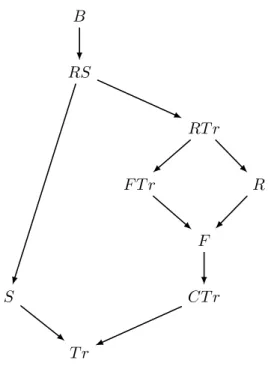
The relations between all the equivalences defined in the previous section are summarized in Figure 2.1, where arrows represent strict inclusions [Gla01].2

B RS RT r F T r R F S CT r T r

Figure 2.1: Spectrum for LTSs

2.2.4 Logical characterizations

In the following chapters, we are going to exploit the logical characterizations of the coin-ductive equivalences that we have defined, in particular for ready simulation equivalence and simulation equivalence. The logical characterization of bisimilarity is given by the Hennessy Milner Logic (HML). The formulas of HML are defined by the following gram-mar: F ::= > ¬F F1∧ F2 h a iF

for a ranging over the labels in a given set A. Given an LTS (S, A, −→), we define the satisfiability of formula F in state s (notation: s |= F ) as follows:

1

We could have equivalently defined failure trace equivalence using the definition of failure trace that allows a failure set at the beginning of the trace as well, and analogously for ready trace equivalence.

2

Standard counterexamples for the strictness of these inclusions will be presented in examples in Chapter 3.

(28)

2.3 Behavioral equivalences for probabilistic processes 27

s |= > always

s |= ¬F iff s 6|= F

s |= F1∧ F2 iff s |= F1 and s |= F2

s |= h a iF iff there is a s0 such that s−→ sa 0 and s0 |= F .

Proposition 2.7 ([HM85]). Let (S, A, −→) be an image finite LTS. For every s1, s2 ∈ S, s1 ∼Bs2 if and only if for every formula F of HML, s1 |= F if and only if s2|= F .

Analogous characterization results, using weaker modal logics, hold for ready simu-lation equivalence and simusimu-lation equivalence. The formulas of Ready Simusimu-lation Logic (RSL) on A are defined as follows:

F ::= > ¬a F1∧ F2 h a iF

In contrast with Hennessy Milner Logic, this logic does not have a full negation operation ¬F , since negation is limited to single (terminal) actions, via the operator ¬a. The satisfiability of ¬a is defined as:

s |= ¬a iff s−→_Xa

The formulas of Simulation Logic (SL) are obtained by removing action negation ¬a from the definition of RSL.

Proposition 2.8 ([Gla01]). Let (S, A, −→) be an image-finite LTS. For every s1, s2 ∈ S, 1. s1 ∼RSs2 if and only if for every formula F of RSL, s1 |= F if and only if s2 |= F

2. s1 ∼Ss2 if and only if for every formula F of SL, s1|= F if and only if s2 |= F

2.3 Behavioral equivalences for probabilistic processes

2.3.1 RPLTS

We start by defining equivalences and preorders on RPLTSs.

Given a transition s−→ ∆, a process sa 0 ∈ S is not reachable from s via that a-transition if ∆(s0) = 0, otherwise it is reachable with probability p = ∆(s0). The reachable states form the support of ∆, i.e., supp(∆) = {s0 ∈ S | ∆(s0_{) > 0}.}

In the RPLTS setting, each state-to-state step of a computation is derived from a state-to-distribution transition s−→ ∆.a

Definition 2.9. Let L = (S, A, −→) be an RPLTS and s, s0 ∈ S. The sequence c def= s0, s1. . . sn−1, sn is a computation of L of length n from s = s0 to s0 = sn labeled by σ = a1, a2...., an if for all i = 1, . . . , n there exists a transition si−1

ai

−→ ∆_i such that si ∈ supp(∆i), with ∆i(si) being the execution probability of the step from si−1 to si via action ai conditioned on the selection of transition si−1

ai

−→ ∆i of L at state si−1. We denote by Cfin(s) the set of finite-length computations from s.

Given a computation c ∈ Cfin(s), its conditional execution probability prob(c) can be defined as the product of the conditional execution probabilities of the individual steps of c. This notion is lifted to a set C ⊆ Cfin(s) of identically labeled computations by letting prob(C) =P

(29)

Let L = (S, A, −→) be an RPLTS and s, s1, s2 ∈ S. The definition of the sets of decorated traces from s is defined as for LTS, but using the definition of computation given above for RPLTSs. We then introduce probabilistic trace-based equivalences on L as follows by analogy with [JS90; HT92]. Instead of only observing the possibility of performing a (decorated) trace, we observe the probability of performing the trace.

• s1 ∼PTrs2 iff prob(C(s1, σ)) = prob(C(s2, σ)) for all σ ∈ A∗.

• s₁ ∼_PCTrs2 iff s1∼PTrs2 and prob(CC(s1, σ)) = prob(CC(s2, σ)) for all σ ∈ A∗.

• s₁ ∼_PFs2 iff prob(F C(s1, ϕ)) = prob(F C(s2, ϕ)) for all ϕ ∈ A∗× 2A.

• s1 ∼PRs2 iff prob(RC(s1, %)) = prob(RC(s2, %)) for all % ∈ A∗× 2A.

• s1 ∼PFTrs2 iff prob(F T C(s1, φ)) = prob(F T C(s2, φ)) for all φ ∈ (A × 2A)∗.

• s1 ∼PRTrs2 iff prob(RT C(s1, ρ)) = prob(RT C(s2, ρ)) for all ρ ∈ (A × 2A)∗.

The corresponding preorders can be defined by using ≤ instead of = in the definitions above, and, for failure trace and ready trace equivalence, by requiring that the initial states have the same ready set.

To define probabilistic bisimilarity and similarity, we first define the lifting function lift() : S × S → D(S) × D(S), which lifts a relation on S to a relation on distributions over S.

Definition 2.10. Given a relation R over a set S and ∆, Θ ∈ D(S), we say that ∆ lift(R) Θ if there is a countable index set I and probability values {pi}i∈I such that the following holds:

• P i∈Ipi= 1 • ∆ =P ipi· dirac(si) • Θ =P ipi· dirac(ti) • for every i ∈ I, siR ti

Definition 2.11. Let L = (S, A, −→) be an RPLTS. A binary relation R on S is a prob-abilistic simulation iff, whenever (s1, s2) ∈ R, then for all a ∈ A it holds that s1

a −→ ∆₁ implies s2

a

−→ ∆2 with (∆1, ∆2) ∈ lift(R) . Relation R is a probabilistic bisimulation if both R and its inverse are probabilistic simulations. Processes s1, s2 ∈ S are proba-bilistic simulation equivalent (s1 ∼PS s2) if there exist two simulations R and R0 such that (s1, s2) ∈ R and (s2, s1) ∈ R0. Processes s1, s2 ∈ S are bisimilar (s1 ∼PB s2), or bisimulation equivalent, if there exists a bisimulation R such that (s1, s2) ∈ R.

Many equivalent definitions of probabilistic bisimilarity have appeared in the literature. We have introduced probabilistic similarity ∼PS and probabilistic bisimilarity ∼PB using the notion of probabilistic lifting of a relation, as in [Den14]. This is analogous to defining simulations and bisimulations using a weight function [JL91; Seg95; Bai98]. As shown in [Seg95], the resulting bisimilarity is equivalent to the one given by the definition by Larsen and Skou in [LS91], which requires a probabilistic bisimulation to be an equivalence relation and uses equivalence classes to compare the reached probability distributions:

(30)

2.3 Behavioral equivalences for probabilistic processes 29

~

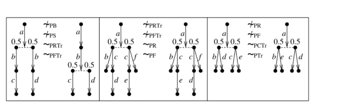
PB

~

PS

~

PRTr

~

PFTr

~

PRTr

~

PFTr

~

PR

~

PF

~

PR

~

PF

~

PTr

~

PCTr a b c 0.5 d 0.5 a 0.5 0.5 c b b d a 0.5 0.5 c e c d b f a 0.5 c d f 0.5 c e b a 0.5 b d 0.5 c e a e 0.5 b 0.5 c d

Figure 2.2: Strictness of inclusions in the spectrum for RPLTSs

An equivalence relation R is a probabilistic bisimulation iff (s1, s2) ∈ R implies that for all a ∈ A it holds that s1−→ ∆a 1 implies s2

a

−→ ∆₂ with ∆1(S0) = ∆2(S0) for all S0 ∈ S/R.

(PB1)

Since the relation is an equivalence, and thereby symmetric, it is not necessary to include the clause from s2 (i.e., s2

a

−→ ∆2 implies s1 a

−→ ∆1 with ∆1(S0) = ∆2(S0) for all S0 ∈ S/R). Requiring a bisimulation to be an equivalence relation is however not convenient when we want to prove that two states are bisimilar, since it requires to build a reflexive, symmetric and transitive relation.

The definitions of probabilistic bisimulation presented so far lead to the same notion of probabilistic bisimilarity. In other words, although the definitions of bisimulation do not coincide (i.e., a relation might be a bisimulation according to one definition, but not according to another one), their unions (i.e., the bisimilarities given by the different notions of bisimulation) all capture the same equivalence relation ∼PB.

When referring to probabilistic systems, we sometimes write bisimulation instead of probabilistic bisimulation, and analogously for the other probabilistic equivalences and preorders. For decorated traces, we also sometimes omit the notation for the specific set of computations when it is clear from the context (e.g., if we are explicitly considering failure traces φ we write prob(s, φ) instead of prob(F T C(s, φ))).

2.3.2 Spectrum for RPLTSs

It was shown in [Bai98; BK00] that ∼PBand ∼PS coincide, hence the variants in between (ready similarity, failure similarity, completed similarity) collapse too. Moreover, the proofs of the results in [JS90; HT92] for fully probabilistic processes can be smoothly adapted to the RPLTS case, and also extended to deal with ∼PRTr and ∼PFTr. As a consequence, we have the following spectrum under the assumption that every state has finitely many outgoing transitions, i.e., it is finitely-branching.

Proposition 2.12. On finitely-branching RPLTS processes, it holds that: ∼PB= ∼PS( ∼PRTr= ∼PFTr( ∼PR= ∼PF( ∼PCTr= ∼PTr

The strictness of all the inclusions above is witnessed by the counterexamples in Fig. 2.2. The graphical conventions for process descriptions are as follows. Vertices represent states and action-labeled edges represent action-labeled transitions. Given a transition s−→ ∆, the corresponding a-labeled edge goes from the vertex for state s to aa set of vertices linked by a dashed line, each of which represents a state s0 ∈ supp(∆) and

(31)

is labeled with ∆(s0). The label ∆(s0) is omitted when it is equal to 1, i.e., when ∆ is the Dirac distribution dirac(s0).

2.3.3 Testing characterizations

On RPLTSs, probabilistic bisimilarity can be captured by considering a simple class of tests. Let T be the language of tests t defined as follows:

t ::= ω

|

a.t

|

(t1, t2)

where a ranges over the labels in the action set A of the RPLTS. The test ω represents success, a.t sequentially checks whether it’s possible to do a and then proceeds with test t, and (t1, t2) is the conjunctive test. Formally, given a reactive probabilistic process s, the probability of success Pr(t, s) when the test t is executed on s is defined by structural induction on t: Pr(ω, s) = 1 Pr(a.t, s) = ( 0 if s 6−→a P s0_∈supp(∆)∆(s0) · Pr(t, s0) if s a −→ ∆ Pr((t1, t2), s) = Pr(t1, s) · Pr(t2, s).

It holds that two processes are bisimilar if and only if, for every test of T, they have the same probability of passing the test.

Theorem 2.13. ([BMOW05]) On reactive probabilistic processes, s ∼PBs0 iff Pr(t, s) = Pr(t, s0) for every test t in T.

The theorem above provides a further simplification of the class of tests defined by Larsen and Skou in [LS91], and proved to characterize probabilistic bisimulation. Indeed, the tests in [LS91] also contain a probabilistic negation operator ¬a restricted to actions, defined as Pr(¬a, s) = ( 0 if s−→a 1 if s 6−→a 2.3.4 NPLTS and resolutions

The definitions of simulation and bisimulation on NPLTSs are the same as on RPLTSs (Definition 2.11). The definition of trace-based equivalences could not be applied directly to NPLTSs, since they rely on the fact that the model has no internal nondeterminism. To extend the definition to NPLTSs, we introduce resolutions, which represent RPLTSs that can be obtained by applying a scheduler (resolving the internal nondeterminism) to the NPLTS under consideration.

Definition 2.14. Let L = (S, A, −→) be an NPLTS and s ∈ S. An NPLTS Z =

(Z, A, −→Z) is a resolution of s if there exists a state correspondence function corrZ : Z → S such that s = corrZ(zs), for some zs∈ Z, and for all z ∈ Z it holds that:

• If z−→a Z∆, then corrZ(z)−→ ∆a 0 with corrZ being injective over supp(∆) and ∆(z0) = ∆0(corrZ(z0)) for all z0 ∈ Z.

(32)

2.4 Calculi 31

• If z a1

−→Z∆1 and z a2

−→Z∆2, then a1 = a2 and ∆1 = ∆2.

We let z_sZ denote the correspondent of s in a resolution Z of s (i.e., s = corrZ(zZs)), and we sometimes simply write zs if the resolution we are referring to is clear from the context.

Z is maximal if, for all z ∈ Z, whenever z has no outgoing transitions, then corrZ(z) has no outgoing transitions either. We respectively denote by Res(s) and Resmax(s) the sets of resolutions and maximal resolutions of s.

As Z ∈ Res(s) is fully probabilistic (i.e., it has no nondeterminism), the probability prob(c) of executing c ∈ Cfin(zs) is the product of the (no longer conditional) execution probabilities of the individual steps of c. This notion is lifted to C ⊆ Cfin(zs) by letting prob(C) =P

c∈Cprob(c) whenever none of the computations in C is a proper prefix of one of the others.

Using resolutions, we can define trace-based equivalences on NPLTSs

Definition 2.15. Let ∼ be any of the trace-based equivalences defined for RPLTSs. Let L = (S, A, −→) be an NPLTS and s, s0 two states of the NPLTS. Then s ∼ s0 if

• for every resolution Z of s there exists a resolution Z0 of s0 such that z_sZ ∼ zZ_s00 (where ∼ is defined as for RPLTSs);

• for every resolution Z0 _{of s}0 _{there exists a resolution Z of s such that z}Z s ∼ zZ

0

s0 (where ∼ is defined as for RPLTSs).

In both items above, the second occurrence of ∼ is defined as for RPLTS, since res-olutions are indeed RPLTS. However, since also external nondeterminism is resolved by resolutions, decorated traces would not be visible. Hence, we assume that failure or ready sets are checked on the states of the original NPLTS. For instance, given a state s in a NPLTS and a resolution Z of s, the probability of zshaving the failure trace (a1a2...an, F ) is the sum of the probabilities of all the computations zs, z1, z2, ...., zn from zs in the res-olution such that the computation is labeled by trace a1a2...an and the correspondent corrZ(zn) of the last state of the computation in the original NPLTS cannot perform any of the actions in F .

The spectrum of equivalences for NPLTS and variations over the definition of resolu-tions (e.g., by considering probabilistic, instead of nondeterministic, schedulers) can be found in [BDL14a; BDL13]. Finally, the probabilistic equivalences considered in this thesis are exact probabilistic equivalences, i.e., we require the observed probabilities to be the same in the compared processes; different approaches allow the probabilities to differ up to some bound p [DLT08].

2.4 Calculi

The terms of pure λ-calculi are generated by the following grammar: M, N ::= x λx.M M N

where x is a variable from a countable set of variables, λx.M is an abstraction and term M N is the application of term M to N . A term M is closed if every variable x occurring

(33)

in M is bound by λx. We identify α-convertible terms. We write M {N_/_x_{} for the} capture-avoiding substitution of N for x in M . The values are the terms of the form λx.M . We use meta-variables M, N . . . for terms, and V, W, . . . for values. When we write terms of the λ-calculus, we use the standard notational convention for parenthesis: abstraction binds to the right and application binds to the left.

A context C is an expression obtained from a term by replacing some subterms with holes of the form [·]i. We write C[M1, . . . , Mn] for the term obtained by replacing each occurrence of [·]i in C with Mi. Note that a context may contain no holes, and therefore any term is a context. The context may bind variables in M1, . . . , Mn; for example, if C = λx.[·]1 and M = x, then C[M ] is λx.x, not λy.x. The indexing of the holes in contexts is usually omitted.

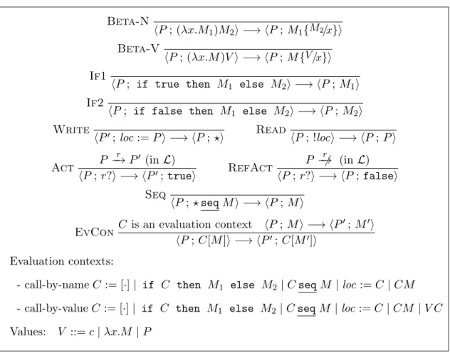
In call-by-name, term M reduces in one step to term N if there is a derivation of M −→ N using the rules Beta-CBN and EvCon in Figure 2.3, using the CBN evaluation contexts. Evaluation contexts, in contrast with standard contexts, may have only one occurrence of a single hole [·]. In call-by-value, one-step reduction is defined analogously, but using rule Beta-CBV and rule EvCon with the CBV evaluation contexts.

The rules are defined using a single-step (or small-step) reduction relation. We write =⇒ for the multi-step reduction relation, defined as the reflexive and transitive closure of −→.

We use a tilde to denote a tuple; for instance, fM is a tuple of terms M1, ..., Mn for some n, and ( fM )i is its i-th element. Hence, we write C[ fM ], with fM = M1, ..., Mn, for C[M1, ..., Mn]. Sometimes we write tuples as {Mi}i when we want to emphasize the indexing set. All notations are extended to tuples componentwise.

We use λ.M to denote a thunked term, i.e., a term λx.M for x a variable not occurring in M .

Beta-CBN

(λx.M )N −→ M {N_/_x_} Beta-CBV _{(λx.M )V −→ M {}V_/_x_} EvCon M −→ N C is an evaluation context

C[M ] −→ C[N ] CBN evaluation contexts C = [·] CM CBV evaluation contexts C = [·] CM V C

(34)

Chapter 3

The discriminating power of

higher-order languages

In this chapter we study the discriminating power offered by higher-order concurrent lan-guages, and contrast this power with those offered by higher-order sequential languages (which are deprived of all concurrency) and by first-order concurrent languages (which are deprived of all higher-order features). The comparison is carried out by considering embeddings of first-order processes into the languages, and then examining the equiva-lences induced by the resulting contextual equivaequiva-lences on the first-order processes. In other words, the discriminating power of a language refers to the existence of appropri-ate contexts of the language that are capable of separating the behaviors of first-order processes.

The higher-order sequential languages are λ-calculi with a store location, akin to im-perative λ-calculi. The λ-calculi offer constructs for reading the content of the location, overriding it, and for performing basic observations on the process stored in the location. The higher-order concurrent languages are HOπ, which allows higher-order communi-cation, and HOπpass, an extension of HOπ with passivation (similar to the languages in [PS12a; KH13; LSS11]). Both languages also admit first-order communications, to be able to interact with the embedded first-order processes. The first-order concurrent language that we consider is CCS−, a CCS-like calculus.

The λ-calculi also allow us to observe the inability for a process to perform a certain action. In concurrency, this possibility is referred to as action refusal. For a thorough comparison, we therefore also consider both restrictions of the λ-calculi without the re-fusal observation (though at the price of allowing computations that may get stuck) and extensions of HOπ, HOπpass, and CCS− with the refusal capability.

Concerning the tested first-order processes, embedded into the above languages, we consider both ordinary LTSs and RPLTSs. We show that, on LTSs, the difference between the discriminating power of HOπ and HOπpass is captured, in the λ-calculi, through the difference between the call-by-name and call-by-value evaluation strategies, both with and without refusals. The correspondence between the HOπpass calculi and the call-by-value λ-calculi appears robust, and is maintained in all scenarios examined. The same does not hold between the HOπ calculi and the call-by-name λ-calculi, whose correspondence breaks on RPLTSs. The case of RPLTSs is more involved also when we consider the first-order language CCS−. For instance, the discriminating power of CCS− is strictly in

(35)

between that of the call-by-name λ-calculus and HOπ. In contrast, the three languages are equally discriminating on LTSs.

We also discuss variations of the above settings. In languages with locations, commu-nication may or may not be affected by spatial proximity. This is the difference between global vs. local communications. This difference is important for the semantics of the languages but, as we shall see, does not impinge on their discriminating power.

The contextual equivalences that we consider are may-like (a test, i.e., a context, is successful on a process if there is at least one successful computation). We also discuss the contextual preorders, and ‘must’ forms of success (all computations are successful). We isolate a few scenarios in which, surprisingly, the may and must forms of contextual equivalence coincide.

Section 3.2 considers the embeddings of LTSs and RPLTSs into λ-calculi. Section 3.3.1 shows the syntax and operational semantics of the concurrent languages (CCS- and HOπ-like), whose discriminating power is studied in Sections 3.4 and 3.5. Section 3.6 discusses variations of the scenarios examined, such as language extensions and must-equivalences. Notation: In examples, we sometimes use a CCS-like notation, with prefixing and choice, to describe the processes of an LTS or RPLTS.

3.1 Contextual equivalences

Given a set of processes as states of an LTS or RPLTS L and an algebraic language AL (i.e., generated by a grammar), we can embed the states in the grammar by first taking a bijection f from the set of states s, s0... to a set of constants P, P0... added to the language, and then defining the behavior of the constants as corresponding to the behavior of the states, i.e., s−→ sa 0_{if and only if f (s) = P} ₋_{→ P}a 0 _{= f (s}0_{). Then we say that the equivalence} induced by AL equates the L processes s1 and s2 if C[f (s1)] and C[f (s2)] behave the same for all contexts C of AL.

Here ‘behave the same’ is formalized as in (‘may’) contextual equivalence: for any P1, P2, C[P1] is as successful as C[P2] with respect to a special success observation, indi-cated with ω. The context C is an AL-expression with a single occurrence of the hole [·] in it.

We use P, Q... to range over the (constants for) processes in the language, corresponding to L processes s, t.... For simplicity, L is used both to denote the LTS or RPLTS of tested first-order processes and to denote the corresponding constants embedded in the language. Moreover, in these tested processes each transition represents a visible action, i.e., there is a corresponding coaction with which the action can synchronize and produce a reduction; the actions available for L do not include the success signal ω. We write AL(L) for the extension of AL with the (constants corresponding to) L processes

In a language AL(L), reductions are represented as τ -transitions−→ (or simply −→, inτ λ-calculi). Each language AL used will have constructs for testing the action capabilities of L processes; thus, the set of action names for L is supposed to appear in the grammar for AL. We emphasize that probabilities may appear in the tested L processes, but they may not appear in the AL languages that test the processes.

The operational semantics of AL(L) will be based on different LTS-like models depend-ing on the nature of L. A finite-length computation c from a term M ∈ AL(L) is successful if each step of c is labeled with τ , the last state of c can perform ω, and no preceding state

(36)

3.2 λ-calculi 35

of c can perform ω. We denote by SC(M ) the set of successful computations from M . In the nondeterministic case, when L is an LTS, the semantic model underlying AL(L) is again an LTS.

Definition 3.1. Let L be an LTS, P1 and P2 two processes of L, and AL an algebraic language. In AL(L):

• P1 is contextually may-less than P2, written P1 ≤LAL P2, if SC(C[P1]) 6= ∅ =⇒ SC(C[P2]) 6= ∅ for all contexts C of AL.

• P1 is contextually may-equivalent to P2, written P1 'LALP2, if P1 ≤LALP2 and P2≤LAL P1.

In the case that L is an RPLTS, the definition of contextual equivalence is more involved because the semantic model underlying AL(L) is a nondeterministic and probabilistic LTS (NPLTS). Hence, we resort to resolutions (Definition 2.14).

The contextual equivalence defined below is inspired by [YL92; JY95; Seg96; DGHM08]. Intuitively, P1 is worse than P2 if, for all contexts C, the maximum probability of reach-ing success in an arbitrary maximal resolution of C[P1] is not greater than the maximum probability of reaching success in an arbitrary maximal resolution of C[P2]. To correctly quantify success, we restrict ourselves to Resτ,max(C[P ]), the set of maximal resolutions obtained from C[P ] by forbidding the execution of actions not resulting in interactions (i.e., τ actions).

Definition 3.2. Let L be an RPLTS, P1 and P2 be two processes of L, and AL be an algebraic language. We say that in AL(L):

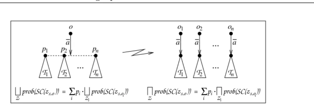
• P1 is contextually may-less than P2, written P1≤LALP2, if for all contexts C of AL it holds that: G Z1∈Resτ,max(C[P1]) prob(SC(zC[P1])) ≤ G Z2∈Resτ,max(C[P2]) prob(SC(zC[P2]))

• P₁ is contextually may-equivalent to P2, written P1 'LALP2, if P1 ≤LALP2 and P2≤LAL P1.

We sometimes abbreviate ‘contextual may equivalence’ as ‘contextual equivalence’ or even ‘may equivalence’.

3.2 λ-calculi

3.2.1 Syntax

Figure 3.1 shows the syntax of the λ-calculus with a location Λloc into which we embed the processes of a (first-order) LTS or RPLTS L. The grammar of the language resulting from the embedding, Λloc(L), has therefore the additional production

Behavioral Equivalences for Higher-Order Languages with Probabilities

HAL Id: tel-01644462

https://hal.inria.fr/tel-01644462

with Probabilities

Valeria Vignudelli

To cite this version:

Alma Mater Studiorum – Universit`

a di Bologna

Behavioral Equivalences for Higher-Order

Languages with Probabilities

Abstract

Acknowledgments

Contents

List of Figures

Chapter 1

Introduction

1.1

Higher-order calculi, concurrency, and probabilities

1.2

Equivalence of programs

1.3

Outline of the thesis

Part I

Discriminating power via testing

equivalences

Chapter 2

Background

2.1

Nondeterministic and probabilistic models

2.2

Behavioral equivalences for nondeterministic processes

2.3

Behavioral equivalences for probabilistic processes

~

~

~

~

~

~

~

~

~

~

~

~

|

|

2.4

Calculi

Chapter 3

The discriminating power of

higher-order languages

3.1

Contextual equivalences

3.2

λ-calculi