HAL Id: hal-01151376
https://hal.archives-ouvertes.fr/hal-01151376
Submitted on 12 May 2015
HAL is a multi-disciplinary open access archive for the deposit and dissemination of sci-entific research documents, whether they are pub-lished or not. The documents may come from teaching and research institutions in France or abroad, or from public or private research centers.
L’archive ouverte pluridisciplinaire HAL, est destinée au dépôt et à la diffusion de documents scientifiques de niveau recherche, publiés ou non, émanant des établissements d’enseignement et de recherche français ou étrangers, des laboratoires publics ou privés.
Extreme Risk, excess return and leverage: the LP
formula
Olivier Le Marois, Julia Mikhalevsky, Raphaël Douady
To cite this version:
Olivier Le Marois, Julia Mikhalevsky, Raphaël Douady. Extreme Risk, excess return and leverage: the LP formula. 2014. �hal-01151376�
Documents de Travail du
Centre d’Economie de la Sorbonne
Extreme Risk, excess return and leverage: LP formula
Olivier LE MAROIS, Julia MIKHALEVSKI, Raphaël DOUADY
Extreme Risk, excess return and leverage: the LP formula
Olivier Le Marois, Julia Mikhalevski, Raphaël DouadyAbstract
The LP formula is based upon the substitution of the exogenous risk aversion hypothesis by a credit equilibrium hypothesis. This leads to a trade-off between expected blue-sky return – the expected return excluding default scenarios – and extreme risk estimated from scenarios leading to default. An empirical study on the past 90 years shows that this trade-off curve is almost identical across asset classes. In equilibrium, an asset expected blue-sky return is proportional to its contribution to extreme risk. Assuming normal returns, we obtain CAPM as a sub-case of the LP relation. This relationship makes extreme risk underestimation a strong driver of asset price bubbles.
Keywords: asset allocation; extreme risk; CAPM; risk budgeting; equilibrium
Olivier Le Marois fluks 25 rue Buffon Paris 75005 France (33) 688338903 [email protected] Julia Mikhalevsky FEDERIS gestion d’actif 20bis rue Lafayette Paris 75009 France (33) 615801970
Raphaël Douady
Labex Refi université Paris I 81 avenue de la République 75011 Paris
This work was achieved through the Laboratory of Excellence on Financial Regulation (Labex ReFi) supported by PRES heSam under the reference ANR-10-LABX-0095.
I. Introduction
Pricing risk has been one of the core topics in quantitative finance for more than half a century. It dates back to the brilliant and sophisticated theory, the Modern Portfolio Theory (MPT), developed by Harry Markowitz in 1950’s. MPT gives a complete answer to optimal portfolio allocation problems, using few assumptions:
1. The goal of portfolio construction is not to maximize returns; it is to maximize returns by unit of variance, while the investor should consider variance of returns undesirable (Markowitz [1952]).
2. There is at least one risk-free asset, whose return is equal to the pure interest rate (Sharpe [1964]).
3. Investors can borrow and lend at equal terms and agree on the prospects of various investments in terms of expected returns, standard deviations and correlations (Sharpe [1964]).
Of course, to quote William Sharpe: “Needless to say, these are highly restrictive and undoubtedly unrealistic assumptions.” But he also added: “However, since the proper test of a theory is not the realism of its assumptions but the acceptability of its implications, and since these assumptions imply equilibrium conditions which form a major part of the classical financial doctrine, it is far from clear why this implication should be rejected.”
Financial markets, however, have dramatically changed and gained in complexity since Markowitz’s seminal paper. Sophisticated financial products, technological advances and growing attention of investors and regulators to extreme risk control, reflected by adoption of UCITS IV, Basel III and Solvency II directives, prompted numerous “post modern” refinements to adapt MPT to the ever-evolving financial markets.
Most of the proposed refinements fit in either of the following two categories:
Replacing variance by more sophisticated risk measures (Rockafellar and Uryasev [2000], Sornette & al. [2000], Rom and Ferguson [1994]).
Replacing return maximization by alternative objective functions (DeMiguel [2009]). However, at the end of the day, only patches keeping MPT’s fundamentals passed the Sharpe acceptability test – such as the Black-Litterman proposition [1992], and passing this test is the key to successfully offering a highly structured and consistent framework for the investment process.
In this article we attempt to answer two fundamental questions that address the value of risk management beyond regulatory compliance:
What is the fair price for risk in terms of short-term performance?
What benefits should the investor expect from risk mitigation in terms of long-term performance?
This article contributes to the risk pricing literature in two ways. We derive an equilibrium relationship between extreme risk and return without making any specific assumptions about asset return distributions or relying on exogenously determined investor utility function. We also show that our risk-pricing model provides rationale for asset price bubbles that were at the heart of the recent financial crises.
II. From Risk Aversion to Bankruptcy Aversion
One of MPT’s most fundamental assumptions is that “investors should consider variance as an undesirable thing” (Markowitz [1952]). Post-modern approach will replace variance by more sophisticated risk measures, such as Value-at-Risk or expected tail loss to name a few. All these approaches have one point in common: they assert that “investors should consider risk as an undesirable thing”
Our proposition is to make tabula rasa of this axiom and state that investors may consider risk as a desirable thing. This might sound counter intuitive, but it is more likely in line with observed investor behavior: after all, taking on more risk allows achieving higher returns, as we shall see below.
On the other hand, to say that most investors consider bankruptcy as a desirable thing not only goes against common sense, but also is not even compatible with the existence of sustainable capitalism. We then have a new assumption on which to build an asset allocation theory: most investors consider bankruptcy as an undesirable thing.
III. Pricing Risk based on Bankruptcy Aversion
Being bankruptcy-averse means that only those with infinite resources can afford to ignore extreme risk. The rest of us have a maximum level of acceptable loss beyond which very unpleasant events start happening, such as bankruptcy and its dramatic consequences: legal/compliance troubles, loss of reputation, unemployment and ultimately misery.
To ban bankruptcy, we need to split the wealth in two portfolios: the Hedge portfolio, which is dedicated to serving liabilities, and the risky portfolio, whose purpose is to produce returns. Of course, the frontier between Hedge and Risky Portfolios is subjective and building an adequate
portfolio has nothing to do with the trade-off between return and risk. It is just a matter of how
future cash flows are discounted and what the perceived risk factors driving the liabilities are, so that the best hedges can be identified.
The trade-off between return and risk results from the risky portfolio management. First, let us observe that a good practice is to host this risky portfolio as a fund, meaning a limited liabilities vehicle, which will invest in risky assets, and finance its investment with equity and debt. The advantage of this fund is that the equity owner can never lose more than 100% of the equity while using debt to increase the capital allocated to the assets, and therefore boosting the equity
excess return vs. the average interest rate charged for the debt. The price paid for this boosted
returns is that more leverage means more risk, i.e. a higher probability to lose 100% of the equity.
The actual return on equity is quantified by Proposition II of Modigliani and Miller’s theorem, ignoring taxes (Modigliani and Miller [1958]):
d
d d e r r r r r E D r r 0 ( 0 ) 0 (1.1)where re is the leveraged return or equity return, r0 is the assets return or unleveraged return, rd is the average cost of debt, D the amount of debt, E the equity and
E D E
the leverage. We see that the leveraged return on equity re depends on 3 variables: the unleveraged asset return r0, the
cost of debt rd and the level of leverage .
To derive the expected equity return, we cannot simply replace realized returns by expected returns in equation (1.1), since the equity owner benefits from an asymmetrical pay-off: the equity loss cannot exceed 100%, while the gain is unlimited. In fact, eq. (1.1) should read:
0
max 1,
e d d
r r
r r (1.2)Given the asymmetrical nature of the equity holder’s payoff, in order to obtain the expected equity return we need to split unleveraged asset return scenarios into 2 categories:
Scenarios leading to fund default. These scenarios happen if the future value of the asset,
r0), falls below the amount to be repaid to the lender (– 1)(1 + rd). This gives the default triggering unleveraged asset loss, that we note VaR() (for reasons to become clear below) as: 1 ( ) rd d VaR r (1.3)
In this case, when r0 –VaR(), the expected equity return is re = –100%, regardless of the amplitude of asset losses. The excess of loss is equal to –(r0 + VaR()) and is supported
solely by the fund’s counterparties and the clearing brokers or exchanges1
.
1
The blue-sky scenarios. These scenarios do not lead to default. In this case the expected
equity return will depend on expected blue-sky return (EBSR), i.e. the expected unleveraged asset return, ignoring all losses higher than the default threshold VaR:
)) ( (r0r0 VaR E
EBSR (1.4)
The expected equity return in this case is obtained by replacing the realized return r0 in equation
(1.1) by the expected blue-sky return:
)) ( ( )) ( (rer0 VaR Erd EBSR rd E (1.5)
If we denote by q the probability of a blue-sky scenario, i.e. of non-default, then the expected equity return becomes, noting that re = –1 in case of default:
0
E( )re qE r re VaR( )
1 q (1.6)The threshold VaR() is clearly a function of the confidence level q: the higher the confidence, the higher the loss threshold. Remembering that the maximum loss an asset will not exceed with a given probability q is exactly the definition of Value-at-Risk, we may denote the unleveraged asset default threshold, as a function of the confidence level q, the Value-at-Risk, VaR(q). Since the default threshold is a function of q, it follows that EBSR can also be expressed as a function of q. Therefore, the expected equity return can be expressed as a function of q, instead of the leverage , according to the following equation, that one obtains after a short calculation (see Appendix 1 for a proof):
( ) ( ) 1 ( ) 1 ( ) e d d EBSR q VaR q E r q r r VaR q (1.7)This relationship establishes the first trade-off between risk and return in our model: the higher the confidence level q, the higher the Value-at-Risk and thus (from equation (1.3)) the lower the leverage and the lower expected equity return. Consequently higher default risk results in lower expected equity return. By the same reasoning we can infer that once the equity investor sets an acceptable level of confidence q, only 3 parameters determine his/her expected return:
- VaR(q), the level of possible loss on the underlying asset,
- EBSR(q), the expected unleveraged gain excluding losses higher than VaR(q), - rd, the cost of debt.
Indeed, the leverage is deduced from the default triggering threshold VaR(q).
IV. Introducing an Efficient Credit Market: the Leveraged Portfolio formula (LP) Up until now we assumed that the confidence level of non-default q was given. In this section we show that this probability is a result of equilibrium in the credit markets.
Let us first consider an investors perspective. An equity owner with a low bankruptcy aversion will choose a confidence level that maximizes equity return. Can equity returns reach an infinite level?
Considering equation (1.7), if the cost of debt rd does not depend on confidence level q, the investor can choose the confidence level q in such a way so that VaR(q) is very low and that the
denominator is close to zero (typically for values of q around 50%), in which case the expected equity return can reach a very high level simply because the leverage is inversely proportional to VaR(q) (equation (1.3)) and will consequently be almost infinite in that case.
Of course, if lenders are rational, they will charge higher interest rates for higher probabilities of default, thus making borrowing unattractive for investors at some point. In other words, the cost of debt is a function of the default probability, which we may write rd(q). The optimal leverage from an investors perspective will therefore be reached when the additional cost of one unit of debt is exactly offset by the additional revenue provided by that unit of debt. From equation (1.7) we know that the investor only considers blue-sky return of unleveraged asset as incremental revenue. As a result, the optimal leverage from an investors perspective is reached when the marginal cost of debt equals the marginal blue-sky return.
From a rational lenders standpoint, the marginal interest rate r qd( ) charged for the latest unit of debt is made up of 2 components:
1r qd( ) 1 rf 1s q( ) (1.8)
rf : a fixed cost of debt, i.e. an interest charge that contains all operational risk factors related to
creditworthiness of the fund management company and which is independent of the level of leverage;
- s(q) : a credit spread that increases with leverage, reflecting higher risk of default due to trading losses for higher levels of leverage.
If the credit market is efficient, this credit spread, charged for one unit of additional debt, should equal the cost of default:
1 1 ( ) (1 ) 0 1 ( ) q q s q q s q q (1.9)We see from equation (1.9) that the lower the confidence q that the fund will survive, the higher the credit spread s(q).
By combining the optimum leverage conditions from an investor perspective with equation (1.9), we can express the market equilibrium in very simple terms: it is reached when the expected
blue-sky excess return over the fixed cost of the debt is exactly equal to the credit spread on the
debt, itself equal to the cost of default (see Appendix 1 for technical proof):
1 * 1 1 ( *) 1 f * EBSR q s q r q (1.10)where q* is the equilibrium confidence level. One could also interpret the probability q* as a risk aversion level, at which the expected blue-sky return EBSR(q) of unleveraged assets exactly offsets the marginal cost of the debt. This equilibrium level can be calculated by solving equation (1.10), or more simply, by stipulating that the expected blue-sky return EBSR is an exogenous variable based on investors’ views on unleveraged assets expected performance, ignoring all the default scenarios.
From now on, we shift from considering the survival probability q as leading variable, to taking
EBSR as leading parameter instead, so that we have:
1 ( ) 1 f r q EBRS EBSR (1.11)<
Then, in order to derive the optimal level of leverage and the expected equity return, we cumulate, unit by unit, the benefit obtained from each additional tranche of debt up to the point where the cost of an additional unit of debt is equal to the expected blue-sky return. This process is illustrated in Figure 1.
The fund will take on additional debt up to the level where the marginal blue-sky return equals the marginal cost of debt, with the black area representing the expected equity return. A higher expected blue-sky return leads to a higher equilibrium level of leverage and thus to a higher expected leveraged equity return. On the other hand, higher default risk will limit access to leverage and result in a lower expected leveraged equity return.
The equilibrium conditions established above allow us to derive the expected leveraged equity return in excess of fixed cost of debt achieved assuming that credit markets are efficient (see Appendix 1 for technical proof):
def ( ) exp 1 1 f ( ) EBSR e f r f E r r dx LP EBSR q EBSR r x VaR q x
(1.12) where:- re is the leveraged equity return - rf is the fixed cost of debt -
x r x q f 1 1is the equilibrium survival probability corresponding to a given expected blue-sky return x
- VaR(q) is the Value-at-Risk of the unleveraged asset, for a given percentile q and a time
horizon H equal to debt maturity.
Figure 1:
Optimal leverage with equilibrium in credit markets. The graph shows the relationship between expected blue-sky return, default risk and optimal leverage.
- EBSR is the expected blue-sky return, i.e. the expected return on the unleveraged asset, ignoring all default scenarios corresponding to losses of the unleveraged asset beyond
VaR(q(EBSR)), where 1 ( ) 1 f r q EBSR EBSR .
The expected long-term return for an investor results from leveraged returns, rolling each period the leverage according to short-term return expectation and extreme risk. For this reason it can be viewed as equal to the leveraged returns as given by the LP function above.
This long-term return potential is driven solely by the distribution of unleveraged asset returns, split in two variables, as shown in Figure 2:
- The expected blue-sky return, i.e. the average return above the default threshold (the blue area in Figure 2). This corresponds precisely to the observed investor behavior: investors tend to ignore scenarios leading to default when estimating return potential of an asset. - Extreme risk represented by a cumulative function of default scenarios (dark area in Figure
2).
Business as usual risk – typically reflected by volatility – has no direct impact on the long-term performance, which seems in contradiction with one of the key fundamentals of MPT. However, by assuming that default risk is only driven by volatility (for instance if the distribution of returns is Gaussian), we can retrieve the relationship between expected return of an asset and its volatility as in MPT.
V. Empirical study: Expected Long Term Returns of traditional asset classes
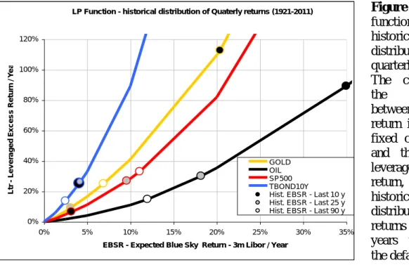
To illustrate the LP function we consider short-term excess returns of 3 different asset classes: equity (S&P 500), bonds (10 year T-notes) and commodities (gold and oil). Using their historical distributions for the past 90 years and different short-term return EBSR0 in excess of fixed cost of
debt as a parameter, we determine by applying the LP function above, the expected long-term excess return as a function of short-term excess return. We took as a fixed cost of debt the 3-month US Libor interest rate.
Figure 2:
Default risk and
blue-sky returns
as determinants of long-term equity return.
Figure 3 below plots this relationship. The three points highlighted on each curve correspond to the realized short-term excess return over the last 10, 25 and 90 year period.
We observe that the slope of the curve is inversely proportional to the extreme risk of the asset, with bonds having the highest slope. In the most recent period the graph clearly shows the commodity bubble as reflected by high short-term excess returns of oil and gold, as well as equities underperformance relative to bonds. It is interesting to note that short-term excess returns calculated over a very long period (90 years) are clustered in the range where there is relatively little variability in values of LP function for different assets; and where the differences in asset extreme risk have less impact on the expected long term leveraged return. By contrast, short-term returns calculated over shorter periods (10 years, for instance) are characterized by much higher variability and thus higher dispersion in expected long-term leveraged excess returns. Intuitively, if we expect a 20% excess short term return for bonds, given much lower extreme risk profile associated with this asset compared to, say S&P500, we would expect a much higher long term excess return achieved through higher leverage.
LP Function - historical distribution of Quaterly returns (1921-2011)
0% 20% 40% 60% 80% 100% 120% 0% 5% 10% 15% 20% 25% 30% 35%
EBSR - Expected Blue Sky Return - 3m Libor / Year
L tr Le v e ra g e d E x c e s s R e tu rn / Y e a r GOLD OIL SP500 TBOND10Y Hist. EBSR - Last 10 y Hist. EBSR - Last 25 y Hist. EBSR - Last 90 y
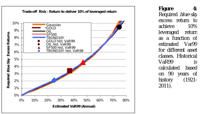
VI. Empirical study: Trade-off between Extreme Risk and Blue-Sky Returns
For a given targeted leveraged return, we can derive a trade-off between short-term return expectation and extreme risk. Unfortunately, there are no simple risk-return ratios to express this trade-off, as the Sharpe ratio, and all its postmodern patches (RORAC, return/expected short fall etc). The reason is that this trade-off involves the entire distribution of default scenarios. Trying to simplify this opens the door to financial products that take advantage of flaws in investment theory, as sub-primes successfully did. Having said that, we can reasonably assume a certain persistence in the shape of tail distributions for risk factors that drive asset returns, provided estimated on sufficiently long historical periods, and therefore derive an empirical trade-off
Figure 3: LP
function applied to historical
distribution of quarterly returns. The chart shows the relationship between blue-sky
return in excess of fixed cost of debt and the expected leveraged excess return, using the historical
distribution of returns over 90 years to estimate the default risk
between expected blue sky short term return EBSR0 and estimated 99% Value-at-Risk, shifting
the tail distribution proportionally.
Trade-off Risk - Return to deliver 10% of leveraged return
0% 1% 2% 3% 4% 5% 6% 7% 8% 9% 10% 0% 10% 20% 30% 40% 50% 60% 70% 80%
Estimated VaR99 (Annual)
R e q u ir e d B lu e S k y E x c e s s R e tu rn s Gaussian GOLD OIL SP500 TBOND10Y GOLD hist. VaR99 OIL hist. VaR99 SP500 hist. VaR99 TBOND10Y hist. VaR99
Continuing the previous example, we can estimate the required blue-sky excess return EBSR0 as
a function of the expected VaR99 level for a given level of targeted leveraged return, in this case 10% per annum, for each asset class. The results are presented in Figure 4.
As expected, higher expected extreme risk will require higher short-term excess return to achieve the same level of expected leveraged performance because of resulting limited access to leverage. For instance, in Figure 4, if for T-Bonds the VaR99 estimation is 25% per year, then it has to deliver a little more than 2% of blue-sky excess return to achieve a 10% leveraged return target. Remarkably, we observe a very similar relationship between extreme risk and required
blue-sky return for all asset classes even though historical VaRs are quite different. We also note
that the Gaussian distribution appears to be a very good proxy for all asset classes. This of course does not imply that asset distributions are Gaussian, just that the trade-off between expected
blue-sky return and extreme risk is similar to that of a Gaussian distribution.
VII. LP formula and the Sharpe acceptability test: the “extended” CAPM
Let us assume as in W. Sharpe seminal paper (Sharpe [1964]), that we are in a fully efficient financial market with rational expectations. In that case, does the LP formula verify the general equilibrium condition as predicted by classical and new classical economic theory?
We can observe that the net market portfolio, which combines hedge portfolios and liabilities, is neutral in respect to factor prices under the homogenous expectations assumptions. To see that, let us imagine that a new pension regime is created, with a stream of future cash flows as
Figure 4: Required blue-sky excess return to achieve 10% leveraged return as a function of estimated Var99 for different asset classes. Historical VaR99 is calculated based on 90 years of history (1921-2011).
liabilities. If markets are efficient and rational, then the forward interest rate will immediately move in response to this anticipation. This movement will be exactly neutralized if the pension plan hedges each dollar of the liability. As a result we can conclude that the hedge portfolio has no impact on asset prices, which are determined solely by the risky portfolio.
As a consequence we can apply the same line of reasoning as in Sharpe’s seminal paper (Sharpe [1964]) and infer that only the aggregate risky portfolio matters for market equilibrium: at the equilibrium all investors will hold a risky portfolio with the same expected LP value (replacing the Sharpe ratio). We can then derive, like W. Sharpe, the expected return distribution of each asset, based on its marginal contribution to the total market expected LP (Appendix 3 provides technical details):
i m f i m f i EBSR r EBSR r w
(1.13)Expression (1.13) is very similar to the fundamental CAPM equation
i f i
m fE r r E r r with 2 major differences:
- The beta in LPT framework is based on the contribution to the extreme risk (see Appendix 3 for details), unlike the CAPM beta that that is estimated from the entire distribution of the returns. This is a very fundamental result: the short-term return that
an asset has to deliver depends solely on its contribution to the extreme risk.
- An asset’s contribution to the blue-sky return of the portfolio is not determined by the
blue-sky return of the asset, but by its expected return conditional on the market default
scenarios not being realized.
This is an intuitive result: investors naturally will split potential returns of an asset in 2 categories: what happens if markets (and not the asset itself) behave normally, and what happens in extreme crisis-like market environment.
The extreme beta calculation in equation (1.13) is considerably simplified if the asset contribution to the market Value-at-Risk is constant in the confidence interval [q*, 1], where q* corresponds to the level of confidence in market equilibrium. In that case, the beta of an asset is exactly equal to the asset contribution to the market Value-at-Risk (see Appendix 3 for technical details): ( *) 1 ( *) i i f i VaR q r VaR q w
(1.14)This observation has very practical key implications for certain class of risk models:
1/ Non linear factor models. In non linear factor models the beta between the asset and the
factors is estimated conditional onfactors return. The beta can then be used to estimate a Value At Risk based on factor distribution quantile with the resulting VaR taking into account the actual tail distribution of the underlying factors as well as tail correlation. In this VaR model, the LPT beta becomes:
i
iw
q
VaR
q
VaR
1
(1.15)This means that the expected contribution of an asset to the blue sky return of the portfolio is proportional to its expected contribution to portfolio VaR, giving here a strong foundation for a VaR-based risk budgeting policy, when accounting for tail correlations.
2/ Gaussian model. If assets returns are jointly log-normally distributed, then an asset
contribution to Value-at-Risk is independent of the level of confidence q and is equal to the asset contribution to the market volatility. The latter is defined as i i
i i Cor w , then in case of a Gaussian distribution: i i Cori
(1.16)This is precisely the definition of the beta in the CAPM: if all assets distributions are Gaussian, then the LPT beta is exactly equal to the CAPM beta.
VIII. Is LP formula sufficiently general?
The discussion in previous sections clearly shows that in LP framework leverage plays a key role in pricing asset risk. A legitimate question to ask then is whether our approach is general enough to be applied to situations where borrowing is restricted.
The investor who has no access to leverage can always choose to invest in a combination of assets that implicitly contains the optimal amount of leverage. One obvious class of assets offering implied leverage is hedge funds, which frequently offer several versions of the underlying fund with different levels of leverage. Another asset class is a company stock: companies finance their assets by a combination of stock and debt, thereby eliminating the need for the shareholder to borrow in order to reach the optimal leverage. Derivative products, in particular listed futures, are a very effective and widely used source of leverage.
Moreover, LP formula relies solely on the assumption that credit markets are efficient in pricing the risk of default, an investor who chooses to borrow to obtain the optimal level of leverage should therefore simply be as efficient as credit markets in order for LP formula to hold.
In conclusion, the price of risk is determined solely by the optimal trade-off between the expected blue-sky return and the distribution of default scenarios. The source of financing, the legal structure of the company or investment payoff type have no bearing on asset long-term return potential.
IX. The cost of bad Extreme Risk estimation
Understanding the consequence of an error in expected return estimation is quite straightforward, and there is no new learning here. Let us therefore assume a hypothetical world of rational
expectations, in which the average blue-sky returns prediction happens to be correct. What about the impact of an error in extreme risk estimation?
Suppose that for a given asset the risk is underestimated, for instance because all market participants use Gaussian model calibrated on a recent blue-sky period. In that case, it means that for a given level of leverage, the probability of default will be underestimated and the spread charged for the leverage will be lower than the true cost of default. Low cost of debt will lead portfolio managers to use excessive leverage and hence to allocate to this asset. This over-allocation will in turn lead to an over-performance of the asset relative to its expected return based on rational expectations models. The potential increase in expected blue-sky returns can lead to an additional increase in the leverage and so on.
As we can see, this risk underestimation will trigger inflation of the asset price relative to other assets (and vs the spreads), i.e. a bubble, initiated by credit that is too cheap and fueled by the resulting excessive demand for the asset. A favorable outcome would be a bubble burst, when lenders realize that the spread they charge is insufficient in real terms and the cost of credit will rise thus bringing asset price to equilibrium. More likely though, the bubble will then turn into an asset price deflation spiral, as lenders shift from risk underestimation to risk overestimation. To quote W. Sharpe: “since the proper test of a theory is not the realism of its assumptions but the acceptability of its implications….”, we can see that LPT gives a rational foundation to sub-prime like crisis and other bubbles fueled by cheap credit and risk underestimation. It also supports most recent macro-economic models, namely those advocated by Hyman Minsky, which give debt accumulation by non-government sector the dominant role in the formation of speculative asset price bubbles (Minsky [1992]).
X. Conclusion
Recent financial crisis raised important questions about the impact of extreme risk budget in asset allocation decisions. In this paper we developed a novel approach to pricing risk, based on bankruptcy aversion and equilibrium in efficient credit markets. We derived an analytical formula, the LP function, that establishes a long term return potential of an asset by combining the blue-sky return expectation on the unleveraged asset and its default risk distribution. Long-term data show that the tradeoff between blue-sky return and extreme risk is remarkably similar across asset classes. By introducing the CAPM hypothesis on market efficiency, we show that at the equilibrium, an asset’s contribution to the market blue-sky return should be proportional to its extreme risk contribution, which, if returns distributions are assumed to be Gaussian, is equivalent to CAPM fundamental theorem.
XI. Appendix 1: Proof of the LP formula
Expected leveraged equity return from investor’s stand point
In this section we derive the relationship between expected equity return, E(re), the confidence level q, the expected asset return conditional on non-default EBSR, the leverage and the cost of debt rd.
Considering the distribution function of the expected unleveraged return, one get can estimate the probability that the fund will not default:
0 0 ( ) VaR q q
r dr
(A1.1)with default threshold defined in equation (1.3):
1 d d r r VaR q (A1.2)The expected equity return defined in equation (1.6) becomes:
( ) 0 0 0 0 0 0 ( )(
1)
( )
1( )
( ) (
1)
1
VaR q e VaR q d dE r
r
r
r dr
r
r dr
q
EBSR q
r
q
(A1.3) with
( ) 0 0 01
( )
VaR qEBSR q
r
r dr
q
.Inserting the default triggering equation (1.3) into the expression for expected equity return, we finally get the expected equity return as a function of the confidence q:
( ) ( ) 1 1 ( ) e d d EBSR q VaR q E r q EBSR q VaR q q r r VaR q (A1.4)Optimal leverage condition
From the investor standpoint, the optimum will be reached when adding more leverage has no impact on his leveraged equity return:
0
0 0 0 0 0 1 ( )e 0 1 d ( ) VaR ( ) VaR E r
r
r
r dr r
r dr
(A1.5)
0 0 0 1 1 f ( ) 1 d 1 0 VaR r VaR r r dr VaR VaR r q
(A1.6)Simplifying we get the required equilibrium relationship:
0 0 0 0 1 1 1 1 1 1 1 f f VaR VaR f f r r dr r dr r q q r EBSR q r s q
(A1.7) LP functionTo derive the LP function let us introduce the following variables: : the excess return vs the fixed cost of debt rf with
f r r 1 1 1 ,
: the excess blue-sky return with 1 1 1 f EBSR r
: the excess risk of unleveraged asset in excess of fixed cost of debt with
1 1 1 f f f r r VaR x v x r The default triggering equation (1.3) becomes:
1
1 s v (A1.8) Differentiating it we get:s
v
dv
d
(A1.9) The expect equity excess return equation becomes:
E
eq
v
1
(A1.10) And the equilibrium equation becomes simply:q q s
1
(A1.11)
Using s as a variable rather than q, and integrating equation (A1.9) we get the relationship between the leverage and the spread:
sx
v
x
dx
Exp
s
v
s
s
01
(A1.12)Inserting (A.11) and (A.12) into (A.10) we get the excess equity return as a function of the
blue-sky excess return and of the excess extreme risk:
1
1
1
0
x
v
x
dx
Exp
LP
E
e (A1.13)Converting back to the absolute return variable, we get:
1 1 f Str e f r f E r r dx q EBSR Exp r x VaR q x
with
x r x q f 1 1 (A1.14)The trade-off between extreme risk and return
If we assume that the shape of default risk is determined by Value-at-Risk with 99% confidence level (VaR99), then we can derive the risk function of unleveraged asset by using different levels of expected VaR99 as a parameter:
1 1 99u q
VaR q VaR (A2.1)
The function u describes the shape of the tail distribution and we assume that it is independent from VaR99, which gives the level of tail distribution.
Typically, the function u can be estimated using historical distributions, in which case taking log of (A2.1) we get:
1
1 99 Ln VaR q u q Ln VaR (A2.2)If we suppose a Gaussian distribution then:
NormInv( ) NormInv(0.99)q
u q (A2.3)
From this we can derive a relation between the blue-sky excess return and VaR99 for a given level of expected equity return:
1 2 1 1 1 1 99 f EBSR e f r u q x dx Ln E r Ln r Ln EBSR x VaR
(A2.4)Extended Sharpe relation
The asset contribution to the market blue-sky return
Let us assume, as in W. Sharpe’s seminal paper (Sharpe [1964]), that all investors face the same cost of fixed debt and have identical views on expected returns and default risk of different assets. In that case, by maximizing expected long-term equity return, all investors choose the same portfolio (“market portfolio”) with identical value of LP function.
The optimal asset weights wi for assets i = 1…n satisfy the following condition at the optimum:
0
i iw
LP
(A3.1)Taking log of (A1.13) and calculating partial derivative with respect to position (i), we get:
1
0
1
1
1
1
1
0 2 0 2
dx
v
x
v
v
v
dx
v
x
v
v
LP
LP
i i i i i (A3.2)This can be written as
i i i w (A3.3) with
0x
v
2dx
w
v
i i i (A3.4) and
v v 1 1 (A3.5) If we convert A3.3 into the absolute return, we get:
i m f i m f i EBSR r EBSR r w (A3.6) Beta calculationWe show in Appendix 3 below that the blue-sky return is homogenous and that
wii1.Then the generic beta expression (A3.4) becomes:
0 2 0 2x
v
dx
v
dx
v
x
w
v
i i i (A3.7)Expressed in absolute returns:
2
2 f f EBSR i i EBSR f i r r VaR q x w r VaR q x EBSR dx dx x VaR q x x VaR q x
with
x r x q f 1 1This formula become much simpler if the contribution of a position to the VaR can be written as
r
VaR
k
w
VaR
f i i i
(A3.9)with ki constant for percentiles superior to q(EBSR). In that case:
r
VaR
w
VaR
f i i i
(A3.10)Blue-sky returns are homogenous
In this section we show that the aggregated blue-sky excess return ε, and hence the absolute return EBSR, is a homogenous but not an additive function.
First let us observe that i i i
w
. That is because when we tilt the position in asset (i) by wi,
the resulting change in blue-sky return of the portfolio will depend on the average return of asset (i) conditional on market, and not asset (i) default scenarios not being realized.
However, as we shall prove below, the blue-sky return is a homogeneous function, meaning that the partial derivatives are additive:
i i i w w
.Based on (A1.3), the market excess blue-sky return is defined as:
d d
qVaR
v1 1 (A3.11) where is the expected excess return of the asset.
If the position i is tilted by dwi and the overall allocation by – dwi (to keep a constant leverage), then the expected excess return of each market scenario will be impacted by
i0
wi.The market blue-sky return
d
d qVaR
v1 1 will hence be impacted in 2 ways: first, the direct impact on the expected blue-sky return assuming the default threshold does not change; second, the impact on market default probability:
i i
v i i i i i w d v v v v w w
2 1 1 (A3.12)From this, we can derive that
v w v w v v d w w w T i i i v i i i i i (A3.13)For each market scenario, the position impact is additive, meaning
0i i
w . The risk function v (the VaR) is homogeneous too, meaning that 0
v w v w i i i , hence T =0, whichXII. References
- Black, Fischer, R. Litterman. “Global Portfolio Optimization.” Financial Analyst Journal, 48 (1992), pp. 28–43.
- DeMiguel, Victor, L. Garlappi, F.J. Nogales, R. Uppal. “A Generalized Approach to Portfolio Optimization: Improving Performance By Constraining Portfolio Norms.” Management Science, 55 (2009), pp.798-812.
- Markowitz, Harry. “Portfolio selection.” The Journal of Finance, 7 (1952), pp. 77-91. - Minsky, Hyman. P. “The Financial Instability Hypothesis.” Working Paper, The
Jerome Levy Economics Institute of Bard College, 1992.
- Modigliani, Franco, M.H. Miller. “The Cost of Capital, Corporate Finance and the Theory of Investment.” American Economic Review, 48 (1958), pp. 261-297.
- Rockafellar, Tyrrell R., S. Uryasev. “Optimization of Conditional Value-at-Risk.” Journal of Risk, 2 (2000), pp. 21-41.
- Rom, Brian M., K.W. Ferguson. “Post-Modern Portfolio Theory Comes of Age.” The Journal of Investing, 3 (1994), pp. 11-18.
- Sharpe, William. “Capital Asset Price, A Theory of Market Equilibrium under Conditions of Risk.” The Journal of Finance, 19 (1964), pp. 425-442.
- Sornette, Didier, P. Simonetti, V.J. Andersen. “φq-field theory for portfolio optimization: “fat tails” and nonlinear correlation.” Physics Reports, 335 (2000), pp.19-92.