Sea-air CO 2 fluxes and carbon transport: A comparison of three ocean general circulation models

HAL Id: hal-03123355

https://hal.archives-ouvertes.fr/hal-03123355

Submitted on 28 Jan 2021

HAL is a multi-disciplinary open access

archive for the deposit and dissemination of

sci-entific research documents, whether they are

pub-lished or not. The documents may come from

teaching and research institutions in France or

abroad, or from public or private research centers.

L’archive ouverte pluridisciplinaire HAL, est

destinée au dépôt et à la diffusion de documents

scientifiques de niveau recherche, publiés ou non,

émanant des établissements d’enseignement et de

recherche français ou étrangers, des laboratoires

publics ou privés.

Sea-air CO 2 fluxes and carbon transport: A comparison

of three ocean general circulation models

J. Sarmiento, P. Monfray, E. Maier-Reimer, O. Aumont, R. Murnane, J. Orr

To cite this version:

J. Sarmiento, P. Monfray, E. Maier-Reimer, O. Aumont, R. Murnane, et al.. Sea-air CO 2 fluxes and

carbon transport: A comparison of three ocean general circulation models. Global Biogeochemical

Cycles, American Geophysical Union, 2000, 14 (4), pp.1267-1281. �10.1029/1999GB900062�.

�hal-03123355�

GLOBAL BIOGEOCHEMICAL CYCLES, VOL. 14, NO. 4, PAGES 1267-1281, DECEMBER 2000

Sea-air CO2 fluxes and carbon transport: A comparison

of three ocean general circulation models

J. L. Sarmiento,

• P. Monfray,

2 E. Maier-Reimer,

30. Aumont,

2 R. J. Murnane,

TM

and J. C. Orr 2

Abstract.

Many

estimates

of the

atmospheric

carbon

budget

suggest

that

most

of the

sink

for

CO2

produced

by fossil

fuel

burning

and

cement

production

must

be in the

Northern

Hemisphere.

Keeling

et al. [ 1989]

hypothesized

that

this

asymmetry

could

be explained

instead

by a northward

preindustrial

transport

of ~ 1 Pg

C y-1

in the

atmosphere

balanced

by an

equal

and

opposite

south-

ward

transport

in the

ocean.

We explore

this

hypothesis

by examining

the

processes

that

deter-

mine

the

magnitude

of the

preindustrial

interhemispheric

flux

of carbon

in three

ocean

carbon

models.

This

study

is part

of the

first

stage

of the

Ocean

Carbon

Model

Intercomparison

Project

organized

by International

Geosphere

Biosphere

Programme

Global

Analysis,

Interpretation,

and

Modelling

Task

Force.

We find

that

the

combination

of interhemispheric

heat

transport

(with

its

associated

carbon

transport),

a finite

gas

exchange,

and

the

biological

pump,

yield

a carbon

flux

of

only

-0.12

to +0.04

Pg

C y-1

across

the

equator

(positive

to the

north).

An important

reason

for

the

low

carbon

transport

is the

decoupling

of the

carbon

flux

from

the

interhemispheric

heat

trans-

port

due

to the

long

sea-air

equilibration

time

for

surface

CO2.

A possible

additional

influence

on

the

interhemispheric

exchange

is oceanic

transport

of carbon

from

rivers.

1. Introduction

The emission of CO 2 to the atmosphere by fossil fuel burn-

ing and

cement

production

averaged

5.4 + 0.5 Pg C y-l during

the decade

of the 1980s. Of this, only 3.2 + 0.1 Pg C y-l re-

mained in the atmosphere. This implies a sink of -2.2 + 0.5

Pg C y-1 in the ocean

and continental

biosphere

[Schimel

et

al., 1995]. An essential problem in global carbon cycle re- search is the partitioning of this sink between the ocean and continental biosphere. Because of the interhemispheric

asymmetry in the land and ocean distribution, much of the re-

search on this issue has centered on the interhemispheric car-

bon budget.

A major constraint is that the observed north-south atmos-

pheric CO2 gradient of-3 ppmv is lower than expected from

fossil CO2 emissions alone. Atmospheric general circulation

models (GCMs) predict that the gradient due to fossil CO 2

emissions should be ~5-6 ppmv (assuming all of it remains in

the atmosphere [Tans et al., 1990; cf. also Law et al., 1996]).

The combined effect of terrestrial and oceanic sources and

sinks, including land use changes such as tropical deforesta- tion, must therefore be to give a larger fossil CO2 sink in the

l Atmospheric and Oceanic Sciences Program, Princeton University,

Princeton, New Jersey.

2 Laboratoire des Sciences du Climat et de l'Environnement, Com-

missariat h l'Energie Atomique, Centre National de la Recherche Scien-

tiffclue

and

Institut

Pierre

Simon

Laplace,

Saclay,

France.

• Max-Planck Instittit far Meteorologie, Hamburg, Germany.

4Now at Risk Prediction Initiative, Bermuda Biological Station for

Research, Inc., Washington, DC.

Copyright 2000 by the American Geophysical Union. Paper number 1999GB900062.

0886-6236/00/1999GB900062512.00

Northern Hemisphere than in the Southern Hemisphere [e.g., Ciais et al., 1995a; Keeling et al., 1989; Tans et al., 1990].

The problem

of accounting

for a large Northern

Hemisphere

sink is exacerbated

by the fact that almost two-thirds

of the

oceanic

sink

of 2 _+

0.8 Pg C y'l predicted

by models

is in the

Southern Hemisphere due to its greater ocean area [Sarmiento et al., 1992]. A further complication is the "rectification" ef- fect, which is the net north-south CO 2 gradient at the surface

that results from the interaction between a seasonally and

diurnally

varying atmospheric

boundary

layer and terrestrial

biosphere

with no net annual

ecosystem

production

[Denning

higher

CO2 in the Northern

Hemisphere

due

to rectification

[Law et al., 1996], which

enhances

the need

for a large North-

ern Hemisphere

sink. However,

the range

in rectification

ob-

tained

by the models

is large, with one even showing

lower

An interhemispheric

asymmetry

in net fossil CO2 sinks

may

be caused

directly

by anthropogenic

perturbations

such

as

deforestation/reforestation and oceanic uptake of anthropo-

genic

carbon

or indirectly

by preindustrial

asymmetries

in

natural

processes.

In the steady

state

carbon

balance

that we

way

to create

such

an asymmetry

is by ocean

transport.

Over

land, the steady

state

assumption

requires

a local balance

of

tions and net organic matter production

and the associated

river transport

of carbon to the ocean [Sarmiento

and

Sundquist,

1992]. Within the ocean,

it is possible

for river

input in one region

to be connected

by ocean

transport

to a re-

Keeling

et al. [1989] proposed

that a preindustrial

transport

of carbon by the thermohaline

circulation

starting in the

1268 SARMIENTO ET AL.: SEA-AIR CO 2 FLUX, A MODEL COMPARISON North Atlantic is the major factor generating the interhemi-

spheric asymmetry in anthropogenic carbon sinks. Tans et al.

[1990], however, concluded that the asymmetry was due pri-

marily to a large terrestrial sink in the boreal midlatitudes.

The sink was attributed to direct anthropogenic perturbations

and the indirect influence of anthropogenic perturbations on terrestrial biota (e.g., nitrogen and CO 2 fertilization). More

recent

analyses

using

13C/12C

and

O2/N

2 ratios

measured

dur-

ing the 1990s have moderated these extreme points of view

[Ciais et al., 1995a; Keeling et al., 1996]; but the problem is still not solved. A major concern in these studies is the diffi-

culty of obtaining reliable long-term averages of the oceanic

behavior.

Analysis

of atmospheric

CO

2 and 13CO2

measure-

ments by Francey et al. [1995] and Keeling et al. [1995] sug- gest large interannual variability in ocean carbon sinks, al- though this is not supported by ocean modeling studies [Le

Qudrd et al., 2000; Winguth et al., 1994]. The approach we

employ here is to use three-dimensional (3-D) ocean carbon cycle models (OCCMs) to estimate the long-term patterns of

oceanic CO 2 sources and sinks, primarily for the preindustrial

state.

A useful reference point for purposes of the present study is

the estimate by Keeling et al. [1989] of a southward transport

of ~1 Pg C y-1 within the ocean

before

the industrial

revolu-

tion. All of this was postulated to occur in the Atlantic Ocean.

Subsequent studies by Broecker and Peng [1992], Keeling and

Peng [1995], and Sarmiento et al. [1995] have examined the

role of the Atlantic thermohaline circulation in generating this interhemispheric transport. They estimated southward

transports

of 0.6, 0.4, and

0.2 Pg C y-l, respectively.

How-

ever, only recently has there been an attempt to explore the global carbon transport including the Indian and Pacific

Oceans [Murnane et al., 1999].

In this paper, we present global model results obtained as part of the first phase of the Ocean Carbon Model Intercom- parison Project (OCMIP-1) organized by IGBP/GAIM. The goal of OCMIP is to improve our capacity to predict the evolu- tion of oceanic carbon uptake and storage by comparison and evaluation of global OCCMs. Experiments dealing with the carbon system have been defined for both the natural cycle and anthropogenic perturbation. In addition, because ocean circu- lation is a major factor controlling the patterns of both the natural and anthropogenic carbon in the ocean, an early focus

of OCMIP has been on the evaluation of the circulation by

tracers

such

as 14CO2

[Orr, 1999].

Two "gradient makers" act to create an inhomogeneous car-

bon distribution in the ocean. The "solubility pump" acts

through sea-air gas exchange at the ocean surface where an at- mosphere-ocean disequilibrium is created by a perturbation in the atmosphere, a heating or cooling of the ocean, or a change in ocean concentrations due to atmosphere-ocean water fluxes and river inflows. The "biological pump" removes inorganic carbon from surface layers during photosynthesis and trans-

ports this carbon

down the water column

before

remineraliza-

tion. It also reduces the surface alkalinity by removing

CaCO3,

which

is counterbalanced

in the deep

ocean

by dissolu-

acts as a "gradient smoother," stirring and homogenizing the

carbon distribution.

We present a set of simulations designed to identify sepa-

rately the contribution of each of the important gradient-

making processes to the present distribution of CO 2 sources

and sinks. The approach we follow is that of Sarmiento et al.

[1995] and Murnane et al. [1999], based on the insights of

Broecker and Peng [1982] and the studies of Volk and Hoffert

[1985], Maier-Reimer and Hasselmann [1987], and Maier- Reimer [1993]. The principal focus of our analysis is the in-

fluence of these processes on the interhemispheric transport

of carbon and the sea-air flux.

2. Model Descriptions

Three groups participated in the full suite of OCMIP-1 re- sults reported here: the Max Planck Institut far Meteorologie

(MPI), Princeton University, and the Institut Pierre Simon

Laplace (IPSL). Table 1 summarizes salient characteristics of the models and gives references. The models differ primarily

in their horizontal and vertical resolution and numerical

schemes. The IPSL model, in particular, has higher horizontal

and vertical resolution than the Princeton or MPI models, and

both the IPSL and MPI models have higher vertical resolution

than the Princeton model. The MPI model uses upstream dif- ferencing, which has large numerical mixing in regions of

high currents. The analyses of Gerdes et al. [ 1991] and Maier-

Reimer et al. [1993] show that the mixing is relatively small

throughout most of the ocean. The analysis of Orr [1999]

shows that the centered differencing scheme used by the

Princeton model gives sea-air fluxes that are virtually identical

to the flux corrected transport multidimensional positive defi-

nite advection transport algorithm (MPDATA) method used in

the IPSL model.

A further important difference in the models is that the IPSL

model uses a semidiagnostic technique in which interior tem-

perature and salinity distributions are forced toward observa-

tions [Aumont et al., 1998; Madec and lmbard, 1996]. All

models use similar geochemistry except for the biological pump. Both the MPI and IPSL models used the prognostic Hamburg Ocean Carbon Cycle Model, Version 3 (HAMOCC-3) parameterization of phosphate utilization described by Maier-

Reimer [1993]. Princeton makes use of phosphate and alka-

linity observations to determine the production and some as- pects of the remineralization [Murnane et al., 1999; Sarmiento et al., 1995]. OCMIP-1 was designed to compare existing

models with a minimum of modification. An ongoing OCMIP- 2 exercise has as one of its elements a simulation using the

same biology in all models to understand better the causes of

differences between models such as those discussed in this pa-

per. Further details of the models are given as each set of

simulations is introduced.

3. Processes

Determining the Sea-Air Flux of

CO2 and Interhemispheric

Transport

In the following

subsections,

we discuss

first a "potential

solubility"

model

that enables

us to directly

compare

the com-

bined

impact

of heat

and

water

fluxes

on the sea-air

CO2

flux in

SARMIE•O ET AL.: SEA-AIR

CO

2 FLUX,

A MODEL

COMPARISON

1269

Table 1. Details

of the Ocean

Carbon

C),cle

Models

Participatinl•

in the Ocean

Carbon

Model

.Intercomparison

Project

Princeton IPSL MPI Model a

Type PE (MOM) PE (OPA7) LSG

Tracer run on-line off-line off-line

Grid

Horizontal 96 x 40 180 x 150 72 x 72

Vertical 12 30 22

Type b B C E

Physics

Forcing prognostic "semidiagnostic" prognostic

Numerics (accuracy) 1st, 2nd 2nd -

Free surface no no yes

Advection scheme centered difference flux corrected transport upstream

Seasonality no yes yes

Mixing c

Vertical explicit Turbulent Kinetic Energy

Model (1.5. order) Horizontal 1000-5000 m 2 s 'l 2000 m 2 s -l Chemistry d Virtual fluxes Biological scheme numerical + explicit 200 m 2 s'l + numerical yes yes no

see text HAMOCC-3 HAMOCC-3

Full descriptions of the models are given by Maier-Reimer [1993] for MPI (Max-Planck Institut), Sarmiento et al. [1995] and Murnane et al. [1999] for Princeton, and Madec and Imbard [1996] and Aumont et al. [1998] for IPSL (Institut Pierre Simon Laplace). The Princeton

OCCM uses the GFDL ocean circulation model as developed by Toggweiler et al. [1989a].

ape indicates primitive equation, MOM is Modular Ocean Model [Pacanowski et al., 1993], OPA7 is Oc6an Parallelis6 version 7, and

LSG is Large-Scale

Geostrophic

inodel.

On-line

and

off-line

refer to whether

the tracer

simulations

were done

simultaneously

with

the

bGrid types are as defined by Arakawa [1972].

CNumerical refers to numerical diffusion caused by the upstream advection scheme.

dCarbon chemistry is as given by Dickson and Goyet [1994] with the CO 2 solubilities of Weiss [1974]. The virtual flux results from the rigid lid approximation in the Princeton and IPSL models, which does not permit water fluxes. Water fluxes are represented instead by a

flux of salt and other tracers [Murnane et al., 1999]. MPI has a free surface that permits water fluxes.

the different models. Biological processes are suppressed. The surface ocean CO2 is forced to be in equilibrium with the atmosphere at all locations. The potential solubility model instantaneously loses CO 2 to the atmosphere in regions where

the combined effect of the heat and water fluxes increases the

CO2 concentration.

It instantaneously

gains CO2 in regions

tion.

In the second "solubility" model, we add a finite "realistic"

gas exchange

to the potential solubility model. The finite

sea-air

gas equilibration

time permits

water to travel over long

or diluted

by the effect

of heat and water

fluxes

and before it re-

equilibrates

with the atmosphere.

This causes

a widening

and

The third topic we discuss

is the effect of biological proc-

esses

estimated

by subtracting

the solubility model from the

"combined" model, which includes both the solubility model

processes

and the biological

pump. An alternative

way to iso-

late the biological

effects

would

be to do a biological simula-

the nonlinearity

of carbon

chemistry,

there is not a single

choice

of temperature

and salinity that would

give an unambi-

guous

measure

of the contribution

of the biological

pump

in

clean

separation

of the two pumps

either. The addition

of bi-

ology

changes

the surface

chemistry

in such

a way as to mod-

ify the response to a given addition or removal of heat or wa-

ter. It would be of interest to compare the two approaches in a

future study.

The biological pump contribution has a zero net sea-air car- bon flux, as it must in a steady state, but there are substantial regional fluxes comparable, in many areas, to the magnitude

of the solubility model fluxes. Thus, the biological pump

substantially alters the spatial distribution of sea-air CO2 fluxes determined by heat and water exchange and by the finite

gas exchange.

Finally, we discuss two additional processes that affect the interhemispheric asymmetry of atmosphere-ocean carbon

fluxes: the river flux of carbon, and the impact of anthropo-

genic CO2 uptake on the spatial distribution of sea-air CO2

fluxes.

3.1. Potential Solubility Model

The potential sea-air flux of CO 2 is defined as the flux that would result if the CO2 content of the surface ocean water equilibrated instantaneously with the atmosphere [cf. Keeling

et al., 1993; Watson et al., 1995]. The equation for the effect

of a flux of heat is:

FCheat=

02 Cp d'•-•=Cp

Q

d[DIC

Q

I1

R

pCO

[DIG]

2 d'••' '

dpCO2/

(1)

where Q is the flux of heat from the atmosphere to the ocean, T

is temperature,

C•, is the heat

capacity

of water,

and

R is the

1270 SARMIE•O ET AL.: SEA-AIR CO 2 FLUX, A MODEL COMPARISON

bon fluxes

is ~1 PW to 0.8 Pg C y-1 for an R of 10 and

dln(pCO2)/dT

= 0.0423

deg

-1 [Takahashi

et al., 1993].

The equation for the effect of a flux of water from the atmos- phere to the ocean (e.g., by evaporation, rainfall, and river

runoff) is

F, water

_{co: = FH:O}

_[DIC]Y

o•

In

pCO2

o•ln[DIC]

o•ln

pCO

2 + •

+ •

Y = o•ln

pCO

2 o•lnS o•ln[Alk]

_=

•-•(1

- 9.4

+ 10)

= 0.16,

where

FH2ois

the flux of water

in m

3 s

'l, S is salinity,

and

from the Geochemical Ocean Sections (GEOSECS) global

mean temperature,

salinity, DIC and Alk obtained

from Taka-

hashi et al., [1981]. The o•lnpCO2/o•ln[Alk]

derivative

in-

water

input

of 1 Sv (106 m

3 s

-1) reduces

the ocean

pCO

2 and

therefore gives rise to a potential CO2 gain from the atmos-

phere

of 0.13 Pg C y-1. A direct

calculation

of ¾

gives

0.17 for

global

mean

properties,

0.18 for average

warm

water in the re-

gion between 45øS and 45øN, and 0.12 for mean cold water poleward of these latitudes.

The MPI and Princeton models are able to diagnose the po-

tential CO2 fluxes directly from (1) and (2) using the heat and

water fluxes in the surface layer of the model. The MPI results

discussed below come from such a calculation. However, the IPSL model has interior sources and sinks of heat and salt that

arise from the semidiagnostic technique used to force model- predicted temperature and salinity toward the observations in

the interior of the ocean. When water parcels affected by these

interior processes outcrop at the surface, their carbon content will be out of equilibrium with the atmosphere even if there is

no in situ sea-air flux of heat or water. In other words, the in-

terior sources and sinks of heat and water masquerade as surface

sources and sinks in their effect on the sea-air CO2 flux. The

only way to estimate the potential CO2 fluxes in the IPSL model is therefore to do an actual "potential solubility" model simulation with equilibration of surface CO2 with the atmos- phere each time step. Note that the sea-air equilibration in an

OCCM simulation cannot be instantaneous owing to the finite

time step. Thus, the surface layer of 10 m thickness in the

IPSL model has a ventilation timescale equal to the time step

of 12 hours. In the Princeton model the potential flux was cal- culated by using (1) and (2), as well as by model simulation with such sea-air equilibration each time step (ventilation time of 1.5 days for the 50 m surface layer). Results from both ap- proaches were virtually identical. The Princeton results given

in this section are from the model simulation.

The potential solubility model used by IPSL and Princeton

solves the full set of carbon system equations. Solving these

equations requires specifying the temperature, salinity, and the

concentration of two carbon system variables. The tempera-

ture and salinity are as predicted by the model. The two carbon system variables used are alkalinity and total carbon. IPSL fixes alkalinity at the observed salinity normalized global

mean

of 2374

lamol

kg

-1 [Takahashi

et al., 1981]. Princeton

o•ln

pCO2.)

(2)

90øS 60øS 30øS 0 ø 30ON 60øN 90øN I , , I , , I , J ] i , I , , I ,

0.16•

h,•

-

o.

121-

1.\',

,

•

-.

...,

... ,

... ,..-..,...

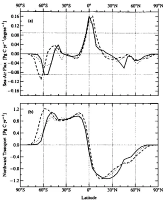
Figure 1. (a) Annual mean sea-air CO2 fluxes from the po- tential solubility model. (b) Annual mean northward CO2 transport in the potential solubility simulation. The solid

line is the IPSL model, the dashed is the MPI model, and the dotted is the Princeton model.

cluded in the potential solubility model, the surface alkalinity

is higher than observed.

The total carbon distribution in the IPSL and Princeton

models is predicted by forcing the surface pCO2 to be in equi-

librium with the preindustrial atmospheric pCO2 of 278 ppm

at each time step. A final steady state total carbon distribution is obtained by running the model forward in time, permitting

the surface total carbon concentrations to propagate into the

interior and gradually modify the initial interior concentra- tions. A steady state solution is achieved when the global in- tegral of the sea-air flux of CO 2 is zero; that is, the interior

concentrations are unchanging. In practice, the models are run

only until the global flux is below a small threshold value. To

achieve this goal, the higher resolution model of IPSL used a

new acceleration technique [Aumont et al., 1998].

Equations (1) and (2) show that the potential sea-air CO2

flux directly reflects the effect of heat and water fluxes across

the sea-air interface. The separate analysis of the impact of Q

and FH20 by Murnane et al. [1999] shows that the heat flux is by far the dominant process in determining the total Fc02 in

the potential solubility model. The discussion in this section thus refers predominantly to features in the heat flux distribu-

tion.

The prominent features of the zonal integral of the sea-air

flux of CO2 are the loss of CO2 to the atmosphere in the trop-

ics and the gain of CO2 in high latitudes of both hemispheres (Figure l a). The loss in the tropics is associated with heating in this region, and the gain in the high latitudes is due to cool- ing. The models follow each other closely except in the

SARMIE•O ET AL.: SEA-AIR

CO

2 FLUX, A MODEL COMPARISON

1271

Table 2. Northward

Transport

of Carbon

at the Equator

Princeton IPSL

Potential Solubility Model

MPI Atlantic -0.50 -0.40 -0.50 Indo-Pacific 0.33 0.17 0.58 Global -0.17 -0.23 0.08 Solubility Model Atlantic -0.24 -0.24 -0.22 Indo-Pacific 0.31 0.24 0.33 Global 0.07 0.00 0.11 Combined Model Atlantic -0.17 -0.18 -0.12 Indo-Pacific 0.05 0.08 0.15 Global -0.12 -0.10 0.04

Combined Model + Bering Strait Contribution a

Atlantic -0.80 -0.81 -0.75 Indo-Pacific 0.68 0.71 0.78 Global -0.12 -0.10 0.04

The transport of carbon is given in Pg C y-1.

aThe carbon transport around the North and South American continents that is

due to the flow through the Bering Strait is estimated to be 0.63 Pg C y-I (P.M.

Haugan and L. Lundberg, personal communication, 1996). Both the IPSL and MPI models simulate this transport directly. The solubility model and combined model re- sults reported above for IPSL and MPI have had this contribution removed.

Southern Ocean, where the MPI model shows a poleward shift

of the region of maximum CO2 uptake and the Princeton model shows a smaller uptake than the other two. The peak uptake

rate of the MPI model in the Southern Ocean is about twice that

of the Princeton model. However, it decreases rapidly to the

north and changes sign at about 55øS, almost 10 ø farther south

than the other two models.

All the potential solubility models predict a small carbon transport across the equator, which is consistent with the

nearly symmetrical sea-air fluxes on both sides of the equator

(Figure lb and Table 2). The southward transport at 15øN is

more

than

1 Pg C y-1 (Table

3), but most

of this is lost to the

large southward transport of carbon in the potential solubility

model would be if there were a substantial net northward trans-

port of heat

or southward

transport

of water. The 1 Pg C

net southward transport hypothesized by Keeling et al. [1989]

would require a cross-equatorial northward heat transport of

~ 1.2 PW.

A variety of observational and modeling studies supports

the notion of a northward cross-equatorial transport of heat in

the Atlantic Ocean [e.g., Martel and Wunsch, 1993; Sarmiento et al., 1995]. The heat transport from our OCCMs implies a

potential

southward

transport

of carbon

of ~0.5 Pg C y-1 in the

net cross-equatorial

transport

is small, about

-0.17 Pg C y-

for Princeton,

-0.23 Pg C y'• for IPSL, and

+0.08 Pg C y-• for

Table 3. Global

Northward

Transport

of Carbon

Princeton IPSL MPI ,,

15øN

Potential solubility model - 1.07 - 1.03 - 1.14 Gas exchange contribution 0.45 0.41 0.67

Biological pump 0.01 -0.05 0.04

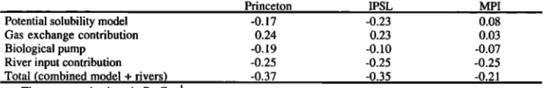
Total (combined model) -0.61 -0.66 -0.43 Equator

Potential solubility model -0.17 -0.23 0.08 Gas exchange contribution 0.24 0.23 0.03

Biological pump -0.19 -0.10 -0.07

Total (combined model) -0.12 -0.10 0.04 15øS

Potential solubility model 1.02 0.97 1.09 Gas exchange contribution -0.23 -0.20 -0.33

Biological pump -0.20 -0.07 -0.26

Total (Combined model) 0.59 0.70 0.50 Potential solubility model

Gas exchange contribution Biological pump

Total (co.mbined model)

30øS

O.88 O.85 O.83 0.11 0.14 0.04 -0.56 -0.22 -0.53 0.43 0.77 0.34

The

transport

is given

in Pg C y'l. The

"gas

exchange

contribution"

is found

by subtracting

the

solubility model from the potential solubility model and thus includes the effect of gas exchange on the solubility pump only. The biological pump is the difference between the combined and solubil-

1272 SARMIENTO ET AL.: SEA-AIR CO2 FLUX, A MODEL COMPARISON

MPI (Table 2). We know of no ocean models with realistic to-

pography and boundary conditions that predict a global cross-

equatorial heat flux of more than a few tenths of a petawatt, in-

cluding the high-resolution world ocean model of Semtner and

Chervin [1992]. Data-based estimates are also mostly small,

giving global cross equatorial heat transports of only a few tenths of a petawatt [Talley, 1984; Hastenrath, 1982; Tren-

berth and Solomon, 1994; cf. Murnane et al., 1999]. The

largest data-based heat fluxes are those obtained by da Silva et

al. [1994], who estimate a northward flux of-0.7 PW in the

Atlantic and-0.7 PW in the Pacific. Combined with a south-

ward flux of-0.7 PW in the Indian Ocean, this study gives a

northward global flux of 0.7 PW. The da Silva et al. [1994] re-

sult is much closer to the value of 1.2 PW required in order to

get a 1 Pg C y-1 southward

flux of carbon. However,

as we

shall see in the following section, the actual solubility pump

carbon transport is much smaller than the potential solubility

pump transport.

The large uptake of CO2 in the Southern Ocean of the MPI

model (Figure l a) requires a correspondingly large northward transport of carbon in the ocean (Figure lb). Note that the CO 2 loss due to heat uptake between 40 ø and 60øS compensates for the CO 2 gain due to the heat loss south of that region. By about 40øS, the northward transport of the MPI model is virtu-

ally identical to that from the Princeton and IPSL models

To summarize, except for the highest latitudes of the South- ern Ocean, the three models included in the potential solubil- ity model comparison have similar zonal integral sea-air CO2 fluxes and meridional CO2 transports. This occurs despite

large

differences

in the model physics. All three models

pre-

this could be increased is if the models predicted a substan-

tially larger northward transport of heat in the global ocean.

This is not supported

by the observations,

most of which

agree

with the ocean

model

results.

Even the larger

da Silva et

-1

y .

3.2. Solubility Model

The solubility model is identical to the potential solubility

model except for the addition of a "realistic" gas exchange

formulation. The atmospheric pCO2 is fixed at its observed

preindustrial value of 278 ppm, and CO 2 is allowed to invade

or evade the ocean until the globally integrated flux is 0. The

IPSL, MPI, and Princeton models all use a modified form of the

wind speed gas exchange coefficient model of Wanninkhof

[1992, equation 5] (with the constant d set to 0.315) with wind

speeds given by J. Boutin and J. Etcheto (personal communi-

cation, 1995). See Orr et al. [2000] for a full explanation.

The equilibration of surface ocean CO2 with the atmosphere

takes of the order of 1 year for a 75 m mixed layer [cf., Broecker and Peng, 1974]. This long delay can lead to a sub-

stantial mismatch between the solubility model fluxes and the

potential solubility model fluxes. For example, the poleward

Ekman transport near the equator rapidly displaces water pole-

ward in both hemispheres before equilibration with the atmos-

phere can occur. This lateral spreading reduces the peak loss

rate at the equator by more than 50% (compare Figures 2a and l a; note the change in vertical scale).

90øS 60øS 30øS 0 ø 30øN 60øN 90øN i i I , , I , J I , , I , , I • , 0.08 - (a) - 0.06 .. .

0.04

0.02

-0.02

[

•" t:

' '"":

- ß

-

,,,.../...

.

S_o.o6|

0.4

0.0

-0.8

Figure 2. (a) Annual mean solubility model sea-air CO2

fluxes. (b) Annual mean northward CO2 transports in the solubility model. The solid line is the IPSL model, the dashed

is the MPI model, and the dotted is the Princeton model.

The gas exchange contribution reduces the southward trans-

port at 15øN by almost 50% (Table 3). Interestingly, the gas

exchange contribution at 15øS is about half that at 15øN (Table

3). This is presumably a result of slower thermocline ventila-

tion (i.e., longer residence times of water in the surface mixed layer) in the southern than in the northern subtropics. The

longer residence time of water in the southern surface mixed

layer permits sea-air equilibration of CO2 to occur, thus bring-

ing the solubility model closer to the potential solubility model results. Note also that the MPI model has a larger gas

exchange contribution at 15øS and 15øN than the other models

(Table 3). This may be caused by the upstream advection scheme used in this model, which can lead to large apparent mixing, i.e., more rapid thermocline ventilation.

The Princeton model has a dip in the CO2 loss at the equator

that is absent from the other models (Figure 2a). The Prince-

ton model differs from the others in that it lacks seasonal forc-

ing. The equatorial minimum in CO 2 reflects the fact that the annual mean wind speeds are substantially lower at the equator than to the north and south. The seasonal migration of the In- ter-Tropical Convergence Zone in the seasonally forced mod- els may be a factor in reducing the influence of this feature.

Another notable feature in the sea-air flux distributions is

that the large uptake peak in the Southern Ocean of the MPI

model has decreased and now looks more like the others (Fig-

ure 2a). Also of interest is the band between -30 ø and 45øS

where the models all show a small loss of CO2 to the atmos- phere in a region where cooling might be expected to lead to CO 2 uptake. In the Princeton model, unusually large upwell-

SARMIENTO ET AL.: SEA-AIR CO 2 FLUX, A MODEL COMPARISON 1273 60øN • 30øN Princeton 30øS

60øS

. ..

120øE 180 ø 120øW 60øW 0 ø 60øE 120øE

60øN . MPI 30øN 30oS 60øS _ 90"S

120"E 180 ø 120øW 60øW 0 ø 60øE 120øE

-4-3-2-1 0 I 2 3 4

90øN

i ....

' ...

'

'

'

IPSL

120øE 180 ø 120øW 600 0 ø60øE 120øE

Plate 1. Maps of annual

mean

sea-air

C02 fluxes

in the solubility

model.

CO

2 to the atmosphere.

The upwelling

is a consequence

of un-

realistically

strong

horizontal

mixing

across

the steeply

slop-

ing isopycnals

of the western

boundary

currents

[Veronis,

1975; Toggweiler et al., 1989b]. The IPSL and MPI models

have similar features.

Maps

of the sea-air

CO2 fluxes

show

that the regions

of

high CO

2 uptake

in the Southern

Ocean

region

of the MPI

model are concentrated in two broad bands near the Ross and

Weddell Seas (Plate 1). The dominant features of the Southern

Ocean

region

of the Princeton

model

are several

regions

of ex-

of all the simulations carried out with the GFDL ocean circula-

tion model using annual mean wind and annual mean surface

temperature

and salinity forcing. They result

from high heat

1274

SARMIENTO

ET AL.: SEA-AIR

CO2

FLUX,

A MODEL

COMPARISON

9t7'N

i

l

120øE 180 ø ! 20øW 60øW O r' 60øE 120øE

60øN . MPI 30øN 30øS 60øS 90øS

120øE 18iT 120"W 60øW O r' 600E 120øE

-4-3-2-1 0 1 2 3 4 60øN 30øN IPSL 3t7'S 6tTS 90øS 120øE 180 ø 1200W 60øW t7' 60•'E

Plate 2. Maps of annual mean sea-air CO2 fluxes due to the biological pump 120øE

loss over convective plumes whose location is fixed. The convective plumes are greatly reduced in versions of the GFDL model that include isopycnal mixing. Note that the convec- tion plumes in the Princeton/GFDL model occur at lower lati-

tudes than the processes that give rise to the peak uptake fea-

tures in the MPI model. The dominant uptake in the Southern

Ocean of the IPSL model is northward of that in the MPI model

and more homogeneous than the convective plume distribu-

tion in the Princeton model.

An interesting

feature

of the IPSL model is the loss of CO2

These occur primarily off the west coast of North and South

America and Africa, as well as a few other regions off

SARMIENTO ET AL.: SEA-AIR GO 2 FLUX, A MODEL COMPARISON 1275 60øN Princeton 30ON x" o 30øS 90øS

120øE 180 ø 120øW 60øW 0 ø 60OE 120øE

90øN

-i

...

120"E 180' 1200W 60"W 0" 60øE 120"E

-4-3-2-1 0 1 2 3 4 60øN

IPSL

Plate 3. Maps of annual mean sea-air C02 fluxes in the combined model. 120"E

likely a consequence of the higher horizontal resolution in the IPSL model. The Princeton model has small uptake maxima at about 35øS and 35øN (most prominent in the potential solubil- ity model, Figure la). These are due primarily to features off

the east coast of Asia, North America, and South America

(Plate 1), where water from lower latitudes is cooled. The IPSL

model shows similar features, particularly in the Northern

Hemisphere. Given the large differences in the regional dis-

tribution of sea-air fluxes (Plate 1), it is remarkable how little

difference one sees in the zonal means (Figure 2a).

The similarity of the solubility simulation sea-air CO2

fluxes of the different models translates into virtually identical

curves of northward carbon transport (Figure 2b). At the equa-

1276

_SARMIENTO

_{ET AL.: SEA-AIR}

_CO

_{2 FLUX,}

_{A MODEL}

_COMPARISON

Princeton models than in the MPI model (Table 3). The cross-

equatorial transport in the solubility simulations of the IPSL

and Princeton

models

is +0.00 and +0.07 Pg C y-1 (northward),

tions

gave

a small

southward

transport

of-0.23 and

-0.17 Pg C

y-i, respectively

(Table

2). The

addition

of a "realistic"

gas

exchange

coefficient

suppresses

a full expression

of the heat

transport

effect

found

in these

two models. This result

sug-

gests

that with realistic

gas exchange

rates

there

is unlikely to

be a 1 PW to 0.8 Pg C y-1 translation

between

interhemi-

spheric

heat transport

and carbon

transport

such

as would

oc-

cur if the gas exchange

between

the atmosphere

and ocean

mixed

layer were instantaneous.

Note that the offsetting

effect

of gas exchange

is particularly

large in the Atlantic Ocean,

where

the southward

transport

of carbon

in the solubility

pump

is about

half that of the potential solubility pump in all

three models (Table 2).

3.3. Biological Pump

The next step in the model comparison study was a "com-

bined"

model

that added

biological

processes

to the solubility

model. Here we discuss the difference between the combined

model and the solubility model, which we ascribe to the influ- ence of the biological pump.

All the biological

models

are based

on phosphorus

cycling.

Production

of organic

carbon

is keyed

to the phosphate

pro-

duction with a stoichiometric C:P ratio of 122 in the

HAMOCC-3 approach used by MPI and IPSL [Maier-Reimer, 1993] and 120 in the Princeton model [Murnane et al., 1999, Sarmiento et al., 1995]. HAMOCC-3 puts newly produced or-

ganic carbon

into particles

that sink instantaneously

and then

are converted to nonsinking particles that remineralize at a

specified temperature dependent rate. The depth distribution of the conversion to nonsinking particles is determined by a sediment trap scaling. Particles that reach the sediments be- come nonsinking particles in the bottom layer in IPSL and en- ter a simple model of diagenesis in MPI. The Princeton model

puts

half the new production

into dissolved

organic

carbon

and

half into particulate

organic

carbon. The dissolved

organic

matter of the Princeton model is remineralized as a first-order

decay process, and the particles sink and remineralize instan-

taneously

according

to a sediment

trap scaling. Particles

reaching

the bottom remineralize

instantaneously

into the

bottom box of the model.

Production

of CaCO

3 in HAMOCC-3 occurs in regions

Princeton

does

not). The CaCO

3 production

is keyed to or-

ganic

carbon,

with a maximum

ratio of 0.5 modified

by a tem-

perature dependent coefficient [Maier-Reimer, 1993]. The

global mean CaCO3 to organic carbon production is 0.22 in

MPI and 0.25 in IPSL. Remineralization

of CaCO

3 occurs

ex-

step by forcing the horizontal

average

of the model

predicted

alkalinity toward its observed value at each depth level

[Murnane et al., 1999, Sarmiento et al., 1995]. The local

model prediction is then made using the global horizontal mean of the ratio of CaCO 3 to organic carbon production and consumption. The export ratio of CaCO 3 to particulate or-

90øS 60øS 30øS 0 o 30øN 60øN 90øN

0.08-

' ' I • , I , , I , , I , , I , ,_•

• 004-

t."• '.

• 0.02- ,.. œ,\

..•.

3

- 0.0 -

'

...'

....

•.2

I-' (b)

• 0,0

.,.':

...

i

...

;....•

'-

-• -0.4

• -08

Figure 3. (a) Annual mean sea-air

CO2 fluxes contributed

by

the biological pump. (b) Annual mean northward CO2 trans-

ports contributed by the biological pump. The solid line is

the IPSL model, the dashed is the MPI model, and the dotted is

the Princeton model.

ganic carbon is 0.26. The export ratio drops to 0.16 if dis- solved organic matter is included. As in previous simulations,

all models predict the atmosphere-ocean balance of CO2 by fixing atmospheric pCO2 at its observed preindustrial value of 278 ppm and allowing it to invade the ocean until the deep

ocean DIC achieves an equilibrium concentration.

The remineralization of organic matter and dissolution of

CaCO 3 produces "excess" dissolved inorganic carbon and nu-

trients in the deep ocean. Most of the excess dissolved inor-

ganic carbon and nutrients are consumed when deep water ar-

rives at the surface. If all of the excess were consumed before

any CO 2 could escape to the atmosphere, the surface ocean and

sea-air flux would look very similar to the solubility model. The only reason for differences between the solubility model and combined model would be that the alkalinity distribution is lower at the surface in the biological pump model. How- ever, there are large regions of the ocean, particularly in the North Atlantic, North Pacific, tropical Pacific, and Southern Ocean, where biological uptake is inefficient relative to the upward supply of excess carbon and nutrients. These regions

lose excess CO2 to the atmosphere (Figures 3a and Plate 2). In

a steady state, this loss must be balanced by uptake in the re- maining regions, namely the subtropics. We thus arrive at the biological pump pattern of Figure 3a and Plate 2. There is a

large loss of CO 2 to the atmosphere in the high latitudes of the

Southern Ocean and a more modest loss in the high latitudes of

the Northern Hemisphere. The IPSL and Princeton models also

have a loss in the tropics. The losses are balanced by uptake in the subtropics.

SARMIENTO ET AL.: SEA-AIR CO2 FLUX, A MODEL COMPARISON 1277 The overall structure of the biological pump sea-air CO 2

fluxes is similar in all three models, but the range between them is greater than in the potential solubility and solubility models. One of the major reasons for the difference between

the IPSL and Princeton models is that the IPSL model has less

convective overturning. This has the consequence that the

biological

pump in IPSL is able to take up a larger fraction of

the nutrients

and excess

carbon brought to the surface

by

lower loss to the atmosphere

than the other models

(Figure

which is half that of the other two biological pump models

(Table 3). Note the different structures in the Southern Ocean

sea-air

CO2 fluxes

of the models,

with a higher

latitude

peak in

different

high latitude convective

overturning

patterns dis-

cussed

previously

(Plate 2), as well as differences

in the way

tio of the MPI and IPSL models is low in the cold waters of the Southern Ocean. The Princeton model has the same ratio there

as elsewhere, which leads to higher CO 2 outgassing.

The loss of excess

biological

pump CO

2 to the atmosphere

in the Southern

Ocean

(Figures

3a and Plate

2) is supplied

by a

-0.19

Pg C y-1 (Table

3). The CO

2 lost to the atmosphere

in

the Southern Ocean comes almost entirely from lower latitudes

of the Southern

Hemisphere.

Note also the small convergence

of carbon

transport

to supply

the flux to the atmosphere

at the

3.4. Combined Model

The outstanding feature of the combined model sea-air flux

is the substantial cancellation of the solubility model fluxes by the biological pump fluxes, The magnitude of the biologi- cal pump sea-air flux is comparable to that of the solubility model, particularly in the Southern Ocean (compare Figures 2a and 3a). The biological pump flux is also of opposite sign to that of the solubility model almost everywhere except the tropics. Consequently, the combined model flux is relatively small everywhere except the tropics (Figure 4a and Plate 3).

The cancellation of the biological pump by the solubility

pump is particularly dramatic in the Southern Ocean, espe- cially in the Princeton model. The wide range between the sea- air fluxes of the three biological pump simulations carries

over into the combined model. The Princeton model has a

large uptake at ~35øS owing to unrealistic upwelling features

along the eastern boundaries of the continents discussed in

Section 3.2. The other two models have a peak uptake at -55øS because the biological pump is not large enough to can-

cel the entire solubility pump.

The sea-air flux features of the combined model are all re-

flected in the carbon transport (Figure 4b). Adding all the con- tributions together, one sees that the total carbon transport across the equator remains small, ranging from -0.12 to +0.04

Pg C y-l (Table

2). All terms

are small

in the MPI model,

but

90øS 60øS 30øS 0 ø 30øN 60øN 90øN 0.08

•'• 0.06

(a)

g, 0.02

v• o.oo

-'- :".'i'/'".'.',

' ....

- ....

• -0 04

• 0.o

:

:

',

...i.

';: ....

...

Figure 4. (a) Annual mean sea-air combined model CO2

fluxes. (b) Annual mean northward CO2 transports in the

combined model. The solid line is the IPSL modeS, the dashed

is the MPI model, and the dotted is the Princeton model.

the Princeton and IPSL models have a relatively large south- ward potential solubility plus biological pump transport

(-0.36

and -0.33 Pg C y-l, respectively)

that is mostly

offset

by the solubility pump gas exchange contribution (0.24 and

0.23 Pg C y-l, respectively).

The transport

at 15øN

is south-

ward in all models but smaller in the MPI model owing primar- ily to the larger gas exchange contribution (more rapid ther- mocline ventilation; Table 3). The transport at 15 ø and 30øS is to the north in all these models but greater in the IPSL model owing to the smaller biological pump contribution dis-

cussed in the previous section.

Table 2 also shows how the basin transports are affected b y

the net water

transport

of 0.8 x 106 m

3 s

'l northward

through

the Bering Strait [Coachman and Aagard, 1988; Roach et al., 1995]. This net water transport gives a northward carbon

transport

of 0.63 Pg C y-1 [Holfort

et al., 1998] that must

be

tration

of 2020 to 2040 },tmol

kg

'l, and

negligible

dissolved

organic carbon [Anderson et al., 1990]. The combined model

transport plus Bering Strait contribution give a very large

southward

transport

of-0.8 Pg C y-1 in the Atlantic Ocean.

terhemispheric transport. The Atlantic Ocean carbon trans-

port estimates of Keeling et al. [1989], Broecker and Peng [1992], and Keeling and Peng [1995] do not include the net carbon transport component due to the Bering Strait through- flow. They should thus be compared with the combined model