HAL Id: hal-03203105
https://hal.archives-ouvertes.fr/hal-03203105
Submitted on 21 Apr 2021
HAL is a multi-disciplinary open access
archive for the deposit and dissemination of
sci-entific research documents, whether they are
pub-lished or not. The documents may come from
teaching and research institutions in France or
abroad, or from public or private research centers.
L’archive ouverte pluridisciplinaire HAL, est
destinée au dépôt et à la diffusion de documents
scientifiques de niveau recherche, publiés ou non,
émanant des établissements d’enseignement et de
recherche français ou étrangers, des laboratoires
publics ou privés.
change of the last deglaciation: a model analysis
Didier M. Roche, H. Renssen, D. Paillard, G. Levavasseur
To cite this version:
Didier M. Roche, H. Renssen, D. Paillard, G. Levavasseur. Deciphering the spatio-temporal complexity
of climate change of the last deglaciation: a model analysis. Climate of the Past, European Geosciences
Union (EGU), 2011, 7 (2), pp.591-602. �10.5194/cp-7-591-2011�. �hal-03203105�
www.clim-past.net/7/591/2011/ doi:10.5194/cp-7-591-2011
© Author(s) 2011. CC Attribution 3.0 License.
Climate
of the Past
Deciphering the spatio-temporal complexity of climate change of the
last deglaciation: a model analysis
D. M. Roche1,2, H. Renssen2, D. Paillard1, and G. Levavasseur1
1Laboratoire des Sciences du Climat et de l’Environnement (LSCE), UMR8212, CEA/INSU-CNRS/UVSQ – Centre d’ ´Etudes
de Saclay CEA-Orme des Merisiers, bat. 701 91191 Gif-sur-Yvette Cedex, France
2Section Climate Change and Landscape Dynamics, Department of Earth Sciences Faculty of Earth and Life Sciences, Vrije
Universiteit Amsterdam De Boelelaan 1085, 1081 HV Amsterdam, The Netherlands Received: 4 November 2010 – Published in Clim. Past Discuss.: 1 December 2010 Revised: 13 May 2011 – Accepted: 16 May 2011 – Published: 9 June 2011
Abstract. Understanding the sequence of events occuring during the last major glacial to interglacial transition (21 ka BP to 9 ka BP) is a challenging task that has the potential to unveil the mechanisms behind large scale climate changes. Though many studies have focused on the understanding of the complex sequence of rapid climatic change that accom-panied or interrupted the deglaciation, few have analysed it in a more theoretical framework with simple forcings. In the following, we address when and where the first significant temperature anomalies appeared when using slow varying forcing of the last deglaciation. We used here coupled tran-sient simulations of the last deglaciation, including ocean, atmosphere and vegetation components to analyse the spa-tial timing of the deglaciation. To keep the analysis in a simple framework, we did not include freshwater forcings that potentially cause rapid climate shifts during that time period. We aimed to disentangle the direct and subsequent response of the climate system to slow forcing and more-over, the location where those changes are more clearly ex-pressed. In a data – modelling comparison perspective, this could help understand the physically plausible phasing be-tween known forcings and recorded climatic changes. Our analysis of climate variability could also help to distinguish deglacial warming signals from internal climate variability. We thus are able to better pinpoint the onset of local deglacia-tion, as defined by the first significant local warming and fur-ther show that fur-there is a large regional variability associated with it, even with the set of slow forcings used here. In our model, the first significant hemispheric warming occurred si-multaneously in the North and in the South and is a direct response to the obliquity forcing.
Correspondence to: D. M. Roche (didier.roche@lsce.ipsl.fr)
1 Introduction
The last deglaciation – '21 to '9 kyrs Before Present (BP) – is Earth’s most recent transition from a glacial-like climate to an interglacial-like climate, a type of transition that oc-cured repeatedly with a periodicity of '100 kyrs over the late Quaternary (Hays et al., 1976; Waelbroeck et al., 2002). Milutin Milankovitch was one of the first to propose that this low-frequency variability of the climate system is linked to the variations of the orbit of the Earth around the Sun, thereby modifying the energy received at the top of the at-mosphere in summer. He proposed that summer insolation at high northern latitudes could be considered as the main driver of the ice-age cycles as it constrained the capacity of winter snow to survive the summer and hence contributed to the buildup of glacial ice-sheets. During peak glacial peri-ods like the Last Glacial Maximum (LGM) most of North America was covered with a '4 km thick ice-sheet (Dyke et al., 2002; Peltier, 2004) and a good part of northern Eu-rope and western Siberia (Svendsen et al., 2004) as well. The orbitally-forced changes in insolation received by the Earth are the only long-term forcing truly external to the Earth’s climatic system, whereas ice-sheet waxing and waning and greenhouse gases that strongly affect the climate over similar time periods are only internal feedbacks to that one forcing. The response of the Earth’s system is non-linear and the ex-act timing of the deglaciation may also be set by a threshold crossing, as is suggested by several authors (Paillard, 1998; Barker et al., 2009; Lamy et al., 2007; Wolff et al., 2009).
Over the years, compelling evidence of how drastic cli-mate changes have been through the last deglaciation have arisen from proxy data retrieved from geological records throughout the world (MARGO Project Members, 2009; North Greenland Ice Core Project members, 2004; EPICA community members, 2004). Although there is no doubt
that this last transition has affected the Earth as a whole, there is still some debate on how changes relate to each other at different geographical locations on Earth (Stott et al., 2007; Huybers and Denton, 2008; Timmermann et al., 2009). Though such debate could in principle be lifted by absolute dating of proxy records and perfect understanding of what is recorded in those proxies, the current science is not there yet. We therefore propose to help with understanding the se-quence of climatic changes of the last deglaciation by per-forming and analysing results from a model simulation to assess within the physical processes contained in our climate model, when, why and where the climate started to warm in an experiment forced by low-frequency variability aris-ing from greenhouse gases, orbital and ice-sheet distribution changes. We also define a time-period in years needed to distinguish between a large local climate change (such as deglaciation) and local interannual or centennial variability.
2 Experimental setup
2.1 Model description
In the present study, we use the LOVECLIM earth system model of intermediate complexity in its version 1.0 (Driess-chaert et al., 2007). In the version applied here, compo-nents for atmosphere (ECBilt), an ocean (CLIO) and veg-etation (VECODE) are activated. It is a follow-up of the ECBilt-CLIO-VECODE coupled model that has been suc-cessful in simulating a wide range of different climates from the Last Glacial Maximum (Roche et al., 2007) to the future (Driesschaert et al., 2007) through the Holocene (Renssen et al., 2005, 2009) and the last millenium (Goosse et al.,
2005). The atmospheric component (ECBilt) is a
quasi-geostrophic model at T21 spectral resolution ('5.6◦in
lati-tude/longitude) with additional parametrizations for the non-geostrophic terms (Opsteegh et al., 1998). ECBilt has three vertical layers in which only the first contains humidity as a prognostic variable. Precipitation is computed from the precipitable water of the first layer and falls in the form of snow if the temperature falls below 0◦C. The time step of in-tegration of ECBilt is 4 h. The oceanic component (CLIO) is a 3-D Oceanic General Circulation Model (Goosse and Fichefet, 1999) run on a rotated B-grid at approximately 3◦×3◦ (lat-lon) resolution. It has a free surface that al-lows the use of real freshwater fluxes, a parametrization of downsloping currents and a realistic bathymetry. CLIO also includes a dynamical-thermodynamical sea-ice component (Fichefet and Morales Maqueda, 1997, 1999) on the same grid. The interactive vegetation component used is VECODE (Brovkin et al., 1997), a simple dynamical model that com-putes two Plant Functional Types (PFT: trees and grass) and a dummy type (bare soil). The vegetation model is resolved on the atmospheric grid (hence at T21 resolution) and allows fractional allocation of PFTs in the same grid cell to account
for the small scale needed by vegetation. The different mod-ules exchange heat, stress and water. It should be noted that there is a precipitation correction needed to avoid the large overestimation of precipitation over the Arctic and the North Atlantic that is present in ECBilt. This surplus of fresh wa-ter is removed from the latwa-ter regions and is added homoge-neously to the North Pacific surface (cf. Goosse et al. (2010) on this aspect). The advantages of the LOVECLIM model when compared to other EMICs are the 3-D oceanic general circulation model and the dynamical atmosphere with actual moisture transport; other models are often energy-moisture balance models.
2.2 Deglacial forcings
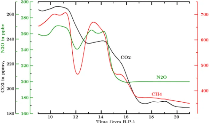
Our goal is to perform a transient simulation of the last deglaciation, from the Last Glacial Maximum (LGM, around 21 kyr BP) to the early phase of the Holocene period (around 9 kyr BP). It shall be noted that there is still some ice present in North America over the Quebec region at this last date; the Northern Hemisphere ice-sheets reaching a near present-day extent around 7 kyrs BP (cf. Renssen et al., 2009, 2010 for an analysis of the impact of the remnants of the Laurentide ice-sheet on the climate evolution of the Holocene). We start our integration at the LGM from the climatic state described in Roche et al. (2007). From 21 kyrs BP onwards, we force the model with insolation changes arising from the long-term changes in orbital parameters (the so-called “Milankovitch forcing”), greenhouse gases changes and ice-sheet distribu-tion, since our model version does not include an interactive ice-sheet component. The orbital parameters are taken from Berger (1978). For greenhouse gases, we prescribe changes in carbon dioxide, methane and nitrous oxide as recorded in air bubbles from ice cores (cf. Fig. 1). Ice-sheet evolution is taken from the ICE-5gV1.2 reconstruction (Peltier, 2004) for both northern and Southern Hemisphere ice-sheets, and inter-polated on the T21 grid of the atmospheric component of our coupled climate model. Between the given ICE-5gV1.2 time slices reconstructions, we linearly interpolate in time with a time step of 50 yr. We both prescribe the orography and ice-mask so as to ensure their joint evolution during the deglacia-tion run, whereas the land-sea mask is kept fixed at LGM. Indeed, it is not obvious how changes in the land-sea mask should be taken into account from the oceanic perspective in order to properly conserve mass, momentum and salinity. Using this approach means that the Barents and Kara seas but also the Hudson bay remain as land throughout and that the Bering strait is kept closed at all times. This means that climatic anomalies in regions like the Bering Strait, the Bar-ents Sea or the Argentinian shelf should be regarded with caution. Similarly, the bathymetry of the ocean was kept to LGM conditions, that is we reduced its depth by 120 m, with a cut-off to the closest vertical model level. This is known to have important implications for the sensitivity of the oceanic
10 12 14 16 18 20 Time (kyrs B.P.) 180 200 220 240 260 CO2 in ppmv, 400 500 600 700 CH4 in ppbv 160 180 200 220 240 260 280 300 N2O in ppbv N2O CH4 CO2
Fig. 1. Greenhouse gas evolution throughout the last deglacia-tion from air measurments on ice-core from both Greenland and Antarctica. CO2is taken from Neftel et al. (1988); Staffelbach et al.
(1991); Inderm¨uhle et al. (1999); Petit et al. (1999); Monnin et al. (2004), CH4from Blunier and Brook (Science); D¨allenbach et al. (2000); Blunier et al. (1995); Chappellaz et al. (1993); Brook et al. (2000); Blunier et al. (1998); Spahni et al. (2005) and N2O from Flueckiger et al. (1999); Spahni et al. (2005). All series are on the EPICA EDC3 timescales and have been smoothed and interpolated on a yearly basis using a cubic spline interpolation scheme for easier use with the model.
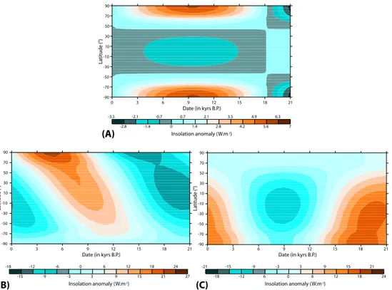
circulation to freshwater fluxes (Shaffer and Bendtsen, 1994; Weijer et al., 2001; Hasumi, 2002; Keigwin and Cook, 2007; Hu et al., 2008). As we focus here on the long-term changes of climate forced by insolation (as shown on Fig. 2 for the annual mean), orography and greenhouse gases in the follow-ing, we should nevertheless capture the first-order changes, though detailed regional features might prove more difficult to interpret.
Finally, in contrast to previous modelling studies of the last deglaciation (Lunt et al., 2006, for example), we do not make use of any acceleration techniques but run the model in real time from 21 kyrs BP to 9 kyrs BP, that is we perform a single run of 12 kyrs duration. This is required in order to properly analyse the phasing of climate change between different locations. Indeed, it has been shown that using ac-celerated techniques tends to bias temperature evolution in regions where the ocean plays a major role, especially in the Southern Ocean and in the Nordic Seas (Lunt et al., 2006; Timm and Timmermann, 2007). Furthermore, as we analyse the relationships between the mean climate change and the interannual-to-centennial variability, we need to use a tran-sient simulation to ensure consistency of timescales in the forcing and response in the climate system.
We would like to stress that while our external forcings are realistic in general, we do not include here freshwater addition to the oceans caused by melting ice sheets. We do not therefore have the forcing needed to reproduce any abrupt climate change during deglaciation. Figure 3 shows a comparison of our modelled temperature at the NorthGRIP ice core site. We have reproduced faithfully the temperature
trend at NorthGRIP until around 16 ka BP, when a sudden cooling in Greenland interrupted the warming trend. This cooling has been associated to the North Atlantic Heinrich Event 1 (cf. Hemming (2004) for a review) that modified the sea surface conditions by the addition of excess freshwater to that area. The subsequent sequence of events was likely responding or forced in the same manner. As we do not in-clude the appropriate forcing for such events, we will focus in the following on the long-term trend in climate in a more abstract framework. A detailed data–model comparison will be the focus of further studies.
3 Analysis method
Analysing climate change throughout the last deglaciation is complex and could be based on different variables (tem-perature, precipitation, etc.). The most obvious change that comes to mind when thinking of deglaciation is warming. We thus chose to concentrate on the phasing of climate evo-lution throughout the last deglaciation, with a focus on the first significant warming occuring after the LGM at every lo-cation. The first significant warming is, a priori, an asyn-chronous event in each grid cell of the model, though some regional patterns are expected to emerge. In reality, this first significant warming would be the first detectable warming in the temperature recorded by any method. In the following, we will define the first significant warming using a statistical test. It requires the knowledge of the “internal” (modeled) variance of the LGM climate, computed here from the last 500 yr of an equilibrium run under constant LGM boundary conditions. Our 12 000 yr deglaciation run is first divided in 120 samples of 100 yr that we tested independently with respect to the control LGM climate. We also performed the analysis with samples of 25 and 200 yr to assess the robust-ness of the method. In the following, we first performed a standard Fischer test on the variances to assess whether they differed or not. When sample variances were equal, we tested the means with a standard Student t-test. When not, we made use of a t-test with two unequal variances defined as (Welsch’s test): testvalue= χref−χsample r σref2 Nref+ σ2 sample Nsample
where χ denotes the mean of the climatic variable over the considered period, N the size (in timesteps) of the period and
σ2 the variance of the climatic variable. “ref” denotes the
reference period (LGM) while “sample” denotes the sample tested against the specified period. From a statistical point of view, the reference LGM period is thus the null hypothesis compared to the deglacial sample considered. In the follow-ing, we consider anomalies that are significant at a 5 % level, that is when tvalue>1.962 for a sample of 100-year
-3.5 -2.8 -2.1 -1.4 -0.7 0 0.7 1.4 2.1 2.8 3.5 4.2 4.9 5.6 6.3 7 -90 -70 -50 -30 -10 10 30 50 70 90 0 3 6 9 12 15 18 21
Date (in kyrs B.P.)
La titude (°) Insolation anomaly (W.m-2) -90 -70 -50 -30 -10 10 30 50 70 90 La titude (°) 0 3 6 9 12 15 18 21
Date (in kyrs B.P.)
-18 -15 -12 -9 -6 -3 0 3 6 9 12 15 18 21 24 27 Insolation anomaly (W.m-2) -90 -70 -50 -30 -10 10 30 50 70 90 La titude (°) 0 3 6 9 12 15 18 21
Date (in kyrs B.P.)
-21 -18 -15 -12 -9 6 -3 0 3 6 9 12 15 18 21 24 Insolation anomaly (W.m-2) (A) (B) (C)
Fig. 2. Insolation anomaly to the 0–30 kyrs BP mean for the last deglaciation computed from Berger (1978) for (A) the annual mean, (B) the northern summer, (C) the northern winter. For (B) and (C) the summer (winter) is computed as the second (fourth) quarter of year after the spring equinox.
less than the mean). We will consider significant temperature anomalies at a given time or the timing of the first significant anomaly as a marker of the local start of the deglaciation pe-riod as modeled with the imposed slow forcings.
4 Results for Surface Air Temperature (SAT) evolution
4.1 Annual mean
In the following we concentrate on a 100-year sample for discussion. Figure 4 introduces the spatial distribution of the timing of first significant warming from 21 ka BP onwards.
The first regions to respond (between 21 and 20 ka BP) are the Arctic Ocean, the northernmost part of Siberia and patches in the Southern Ocean. These are regions affected by the presence of sea-ice, or neighbouring continental re-gions. The first response is immediatedly followed (20 to 19 ka BP) by a significant response of all latitudes poleward
of 35◦ north and south. During that given period of time,
the only forcing is the orbital forcing, greenhouse gases and
ice-sheet forcing being quasi constant (CO2 concentration
changes are '5 ppm). Sea-ice being sensitive to the total amount of energy received throughout the year, increasing the energy received in any season will limit (or even reduce) the sea-ice extent and the buffering effect of the underly-ing ocean will extend (in time) the anomaly to a year-round
Time (yrs BP) -42.5 -40 -37.5 -35 -32.5 -30
Annual mean temperature (Model, °C)
-45 -42.5 -40 -37.5 -35
d18O in ice (NGRIP ice core, per mil)
10 15 20
Time (kyrs BP)
Fig. 3. General outline of the deglaciation simulation: comparison of the modelled annual temperature (yellow) at North Grip (North Greenland Ice Core Project members, 2004) to the North Grip δ18O record (black). The δ18O of the ice is scaled so as to have a 10◦C warming during the Bølling period.
effect. The early response seen in the northern North Atlantic and adjacent regions is therefore an effect of the obliquity in-crease during the early part of the deglaciation that inin-creases the total amount of energy received by the Earth at high lat-itudes, as depicted in Fig. 2. The fact that the early signifi-cant warmings observed in the model are obliquity-driven is further reinforced by the in-phase changes of the Northern
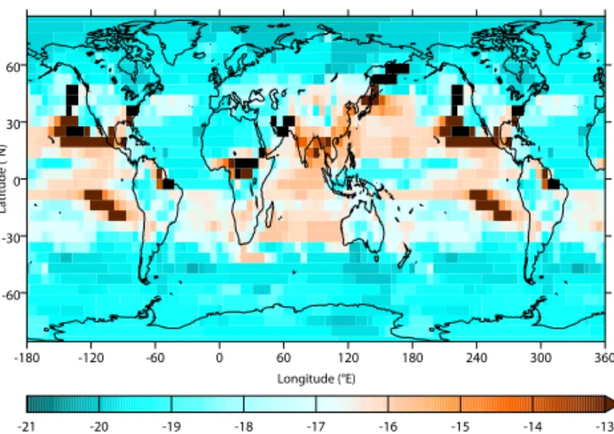
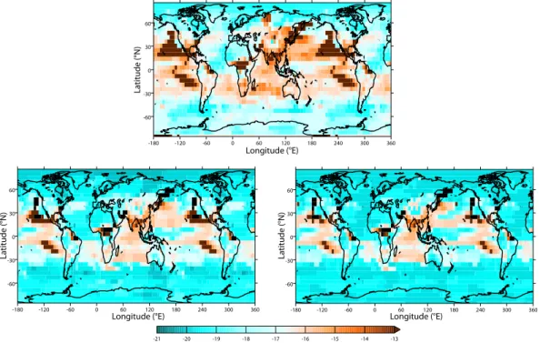
-21 -20 -19 -18 -17 -16 -15 -14 -13 -180 -120 -60 0 60 120 180 240 300 360 -60 -30 0 30 60 Longitude (°E) La titude (°N)
Fig. 4. Timing of first significant warming during the deglaciation from a 100 yr sample at 5 % significance. Color scale is the date in kyrs BP Black denotes regions without significant warming over the deglaciation.
and Southern Hemispheres. This warming is accompanied by a reduction in the sea-ice extent around Antarctica, a re-sult found in other simulations of the last deglaciation (Tim-mermann et al., 2009). We do not find any delay between the Northern and Southern Hemisphere reponses in our model. The sea-ice change in the South therefore responds primarily to the local orbital (obliquity) forcing and not to a delayed response to the North Atlantic warming through upwelled waters as found for other climatic periods (Duplessy et al., 2007; Renssen et al., 2010). By increasing the total energy received from the sun at high latitudes, the obliquity signal forces an in-phase response of both hemispheres at high lati-tudes regions (cf. Fig. 2).
A later response (17 to 15 ka BP) is then observed in most oceanic tropical regions. Given the simplified representation of the physical equations for motion in the atmospheric part of our model, caution is needed in interpreting this pattern. We observe some changes in the precipitation pattern at the same time (cf. Sect. 4.3) that may be linked to ITCZ changes in response to the changing Equator-to-pole gradient as well as change in ice-sheet topography. However, a precise as-sessment of what is occuring in the tropics would require a model with more complex atmospheric physics (Khodri et al., 2009). The time period around 16 ka BP is also a pe-riod when the global greenhouse gas forcing starts to become
significant (CO2 at around 220 ppm, cf. Fig. 1) enough to
counterbalance the obliquity-induced cooling of the tropics (cf. Fig. 2). The later response of the tropical regions are also due to the rather small absolute temperature changes from 21 to 9 ka BP (cf. Fig. 5). It is therefore difficult to discriminate between a small temperature change and year-to-year vari-ability within the model in such areas. Two different types of regions are lagging the response of the rest of the planet.
-6 -3 0 3 6 9 12 15 18 21 24 27 30 33 36 -180 -120 -60 0 60 120 180 240 300 360 -60 -30 0 30 60 Longitude (°E) La titude (°N)
Fig. 5. Annual mean temperature difference (in◦C) between 9 ka BP wrt 21 ka BP for a 100-year sample. Color scale is in◦C.
The first type are areas where the year-to-year variability – as characterized by the sample variance – is higher during the deglaciation and the local temperature change over the deglaciation is not that large. Thus, the deglacial warming becomes significant only late in the deglaciation. Character-istic examples are the continental regions of India and China and the tropical Pacific ocean, becoming significant only af-ter 15 ka BP (with the notable exception of the Himalayas). Figure 6 shows the temperature simulated for one location in
the Pacific Ocean (15◦N, 120◦W) for the LGM and 9 ka BP
The two density distributions are relatively well separated, but not to a 5 % significance level. The deglacial sample has a larger variance (variability) than the glacial one, as charac-terized by the width of the density peak. Within the sample, some years cannot be statistically distinguished from one an-other as for example a series of 20 yr between years 20 and 40. Thus, one can argue that the climate depicted by those two samples is not very different at a 5 % confidence level, i.e. a relatively high confidence level.
The second type are regions where the deglacial warm-ing from 21 ka to 9 ka is never significant (shown by black shading on Fig. 4). They are located in equatorial regions in Africa and south America, offshore California in the north-ern tropical Parific Ocean and in the sea of Okhotsk. These regions are simulated to be colder on an annual mean at 9 ka BP than during the LGM (cf. Fig. 5) and thus never encounter lasting, significant deglacial warming.
4.2 Seasonal means
To pursue a more in-depth analysis on the complex sea-sonal timing of deglacial warming, Fig. 7 presents results for December-January-February (DJF, northern winter) and June-July-August (JJA, northern summer).
DJF shows the largest areas of non-significant warming over the deglaciation. The reason for this is similar to the late warming previously described, i.e. the local variability is too
0 20 40 60 80 100
Time (yr) 0.0 0.5 1.0 1.5 2.0 2.5 3.0Density
25.2 25.4 25.6 25.8 26.0 26.2 26.4 26.6 Temper atur e (°C )
Fig. 6. Comparison of two temperature samples from the deglacia-tion in the Pacific Ocean, offshore Mexico (15◦N, 120◦W). The left panel shows the annual mean temperature evolution over a 100-year sample taken from the reference LGM run (in red) and from the deglaciation (at 12 ka BP, in blue). The right panel shows the density function associated to that sample on the same temperature axis. The dashed vertical lines in the right panel show the means of the series, the filled areas are the respective intervals corresponding to the standard deviations of each series (±σ ).
high for the local warming to become statistically significant. This may be interpreted as regions where a 100-year mean is more representative of interannual to decadal variability than of climate in the sense of a 30-year mean. The time-length of the sample needed for the warming to become significant during the transition is discussed in Sect. 4.4. For a relatively large area centered on the Bering Strait as well as for the Gulf of Mexico, there is no significant warming in DJF at 9 ka BP relative to the LGM as the two regions are significantly cool-ing in our model. Other large areas of non-significant warm-ing (part of the eastern Pacific, continental tropical regions and eastern Eurasia) are characterized by small temperature
anomalies as a whole (below 1◦C in DJF), a change that is
hardly significant with respect to the model interannual vari-ability in the same regions. We nonetheless note the early response of sea-ice regions, first in the northern North At-lantic (19 ka BP) and of the Southern Ocean sea-ice north of
60◦S, better marked than in the yearly mean. Conversely,
JJA shows the smallest non-significant warming from 21 k to 9 k. A striking feature is that most regions have a signif-icant warming early in the deglaciation mostly before 18 ka BP Three large areas are standing out as being earlier than that: the northern North Atlantic, the Southern Ocean around
60◦S and the northern Equatorial regions. The first is due
to sea-ice changes and circulation changes as was noted be-fore, followed by the neighbouring Arctic. Accordingly, the Southern Ocean region is linked to shrinking sea-ice winter extent. -180 -120 -60 0 60 120 180 240 300 360 -60 -30 0 30 60 (DJF) (JJA) -21 -20 -19 -18 -17 -16 -15 -14 -13 -180 -120 -60 0 60 120 180 240 300 360 -60 -30 0 30 60 Longitude (°E) La titude (°N) Longitude (°E) La titude (°N)
Fig. 7. Timing of first significant warming during the deglacia-tion from a 100 yr sample at 5 % significance. DJF (top) and JJA (bottom). Color scale is the date in kyrs BP Black denotes regions without significant warming over the deglaciation.
4.3 Precipitation evolution
Not all proxies for climate change are primarily sensitive to temperature changes during the last deglaciation. The same is true for specific regions, for instance the intertrop-ical regions, where the main response to the last deglaciation is likely to be a change in annual precipitation, not annual warming (Roche et al., 2007). Performing the same kind of analysis, we obtain a geographical distribution of the signif-icant increase (decrease) in precipitation. It should be noted that the precipitation distribution is not normally distributed, but that the logarithm of precipitation is (Vrac et al., 2007). The analysis performed in this section is thus comparable to the previous ones using the logarithm of precipitation as a variable. To simplify the interpretation, we also mask the re-gions where precipitation changes are significant for both an increase and a decrease. That is, we retain areas where there is only an increase (or decrease) in precipitation throughout the deglaciation. The complete sequence of events from the precipitation point of view would require a dedicated study involving an analysis of the Intertropical Convergence Zone (ITCZ) movements through time.
The annual mean precipitation (Fig. 8) shows a significant decrease in a zonal belt in the southern equatorial regions during 20 and 16 kyrs BP. This pattern is due to the north-ward shift of the ITCZ in response to the warmer climate conditions. Indeed, under LGM climate conditions, most models simulate a southward shift of the ITCZ in response to the imposed boundary conditions (Braconnot et al., 2007), a shift consistent with data evidence (Leduc et al., 2007). This shift was shown to respond primarily to global tem-perature changes (Khodri et al., 2009). As the beginning of the deglaciation (21–16 kyrs BP) is marked by relatively low greenhouse gases changes, we observe an ITCZ shift mainly in response to the change in insolation forcing.
The annual mean figure for a significant increase in precip-itation shows a more complex pattern. We can note that there are many more areas with increased precipitation than with decreased precipitation. Indeed, as the atmosphere warms during deglaciation, it can hold more moisture. The global LGM to early Holocene change in moisture content is thus towards an increase, thus leading to an increase in precipita-tion. We can distinguish four different areas. First is the very early change over the Arctic regions; during the LGM these regions are very dry. Thus, a small increase in precipitation at the start of deglaciation is immediatedly significant. Sec-ond, the northern equatorial regions show a relatively zonal pattern; the latter is a counterpart of the decrease seen in the southern equatorial regions and is likely responding to the same ITCZ shift. The timing of this increase is coher-ent with the decrease seen previously. Third, the southern mid-latitudes consistently show an increase in precipitation between 20 and 16 kyrs BP. This is coherent with the regions previously identified in the temperature fields as early
warm-ing (around 60◦S) and bears a link to seasonnal changes in
the sea-ice field. Fourth, the desertic and semi-desertic re-gions (Sahara, Arabia, Pakistan etc.) display an increase in precipitation starting 17–16 kyrs BP. This pattern is generally consistent with an observed transition to more humid con-ditions in northern Africa (Gasse, 2000; deMenocal et al., 2000; Tjallingii et al., 2008; Timm et al., 2010) in response to warmer conditions. However, the role of abrupt events of the last deglaciation (that we do not take into account) calls for caution on the exact timing of the increase.
4.4 Impact of interannual variability
As noted before, our results are sensitive to the sample size used in the study. Indeed, increasing the sample size compar-atively reduces the effect of noise (variability) in the model on the definition of the mean temperature of the sample. A large sample is thus less affected by a series of years with temperature above the mean than a smaller sample. Using a small sample size (e.g. 25 yr), our results therefore empha-size the potential for interannual variability anomalies to be significant at a long-term scale (deglaciation scale). Using different sample size (25, 100, and 200 yr in the following),
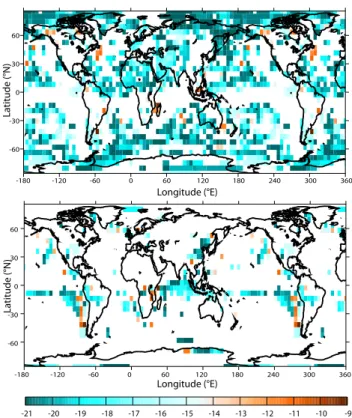
-180 -120 -60 0 60 120 180 240 300 360 -60 -30 0 30 60 -180 -120 -60 0 60 120 180 240 300 360 -60 -30 0 30 60 -21 -20 -19 -18 -17 -16 -15 -14 -13 -12 -11 -10 -9 Longitude (°E) La titude (°N) Longitude (°E) La titude (°N)
Fig. 8. Timing of the first significant annual mean precipitation in-crease (top) and dein-crease during deglaciation from a 100 yr sample at 5 % significance. Color scale is the date in kyrs BP. White areas are locations where precipitations changes are either never signifi-cant or did change signifisignifi-cantly in both increase and decrease.
we may truly assess what is the timing of climate change in the model and decipher regions where the interannual vari-ability is too large to allow significant climatic anomalies on those longer timescales. Figure 9 compares the timing of first significant warming for four different samples of increasing size.
An evident feature arising from Fig. 9 is that a shorter sample yields generally a later significant warming. This re-sults from the fact that the value of the Welch’s test depends strongly on the sample size to determine the significance of the anomaly: If the sample is relatively small and the vari-ability within the sample is large or larger than the reference period, then a larger temperature anomaly is needed to stand out compared to the local variability (cf. Welsch’s test equa-tion). Increasing the sample size thus decreases the impor-tance of the internal variability over the signal and enables a more accurate determination of the first significant, exter-nally forced, warming. In simpler terms, this can be preted as looking at climate compared to looking at inter-nal high-frequency variability: With a small sample having a large variability, one needs a very different sample mean to be significantly different from the reference.
Most interestingly, the size of the sample needed to discuss the climate anomaly versus the reference climate is variable
-180 -120 -60 0 60 120 180 240 300 360 -60 -30 0 30 60 -21 -20 -19 -18 -17 -16 -15 -14 -13 -180 -120 -60 0 60 120 180 240 300 360 -60 -30 0 30 60 -180 -120 -60 0 60 120 180 240 300 360 -60 -30 0 30 60 Longitude (°E) La titude (°N) Longitude (°E) La titude (°N) Longitude (°E) La titude (°N)
Fig. 9. Impact on sample size on the timing of the first significant temperature warming during deglaciation. From top left to bottom right the sample sizes are: 25 (top), 100 (bottom left) and 200 (bottom right) years. Color scale is the date in kyrs BP. Black denotes regions without significant warming over the deglaciation.
spatially. Indeed, both the absolute temperature anomaly and local temperature variability vary in space. Two examples can be taken from Fig. 9 to highlight this feature.
1. In the northern tropical regions over the Pacific and southwestern North America, the total temperature anomalies from 21 ka BP to 9 ka BP (cf. Fig. 5) are
rel-atively small in our model, below 2◦C. Distinguishing
those small anomalies from a larger interannual vari-ability (that is in a sample with a large variance) is there-fore difficult and requires a larger sample. One can note that even with a 200-year sample, not every location in those areas is significantly warmer at 9 ka BP than at LGM.
2. Most regions of central Asia become significantly warmer only late in deglaciation using a 25-year sam-ple. In this case, this is not solely the effect of a small LGM to 9 ka BP temperature difference (some areas
have a temperature anomaly of about 10◦C) but because
of very large variance within the sample, related to high interannual to centennial variability. In fact, the vari-ance of the samples during deglaciation are systemati-cally higher than those of the reference run, making it harder to decipher a climate change from internal high-frequency variability (noise). It should be noted also that the sample size strongly affects the date of first sig-nificant anomaly in this area: Central Asia is sigsig-nificant in the 25-year sample only at 14 ka BP, is significant
between 17 and 15 ka BP in the 100-year sample and around 18 ka BP in the 200-year sample.
The analysis of Fig. 9 confirms our previous inferences that there are three main areas with leading temperature changes: the northern North Atlantic, a north Equatorial band and the
Southern Ocean between 45 and 60◦S.
5 Discussion
Our study so far focusses on a single 12 000 yr run with slow forcings included. To reproduce the effects of millennial-scale climate variability, the modeling study would require the use of higher frequency forcings, such as freshwa-ter fluxes from melting ice-sheets, or understanding how the response to slow forcings can act to produce abrupt events through the non-linearities of the climate system as is recorded in many different proxies (North Greenland Ice Core Project members, 2004; Shackleton et al., 2000; Wang et al., 2001; von Grafenstein et al., 1999, for example). How could we proceed to better determine the response of our cli-mate model to the (imposed) slow forcings? One often-used method (Goosse et al., 2005, for example) is to perform en-semble simulations with identical forcings, varying only the initial conditions. The different expression of the internal variability of the model in the different ensemble members would then cancel out in the mean, leading to a more ro-bust response of the forced response. However, changing our
approach of temporal samples to ensemble samples would require 100 simulations of the full deglaciation period. This is difficult to obtain due to computational constraints. We are thus limited to a single run for the time being.
Natural (observed) climate, on the other hand, is only one trajectory out of many possible solutions. Analysing a single simulation is therefore close to what is recorded by proxy data, albeit that we have a perfect recording of our simulated climate within our idealized “model world”, as opposed to the imperfect recording of the Earth’s climate in proxy data. We have shown that even with perfect recording of the simu-lated climate, there are regions where distinguishing between the deglaciation warming and local variability is problem-atic. Depending on the resolution of the signal recorded in the proxy, a similar issue may arise. What we show from our model simulations is that when the signal is very noisy, high temporal resolution is safer to determine variability and climate evolution. However, high resolution is practically limited by the type of proxy record chosen. For example,
recording δ18O in oceanic sediment cores from foraminifera
have a maximal practical resolution of about ten years for glacial periods (depending on foraminifera abundance, sed-imentation rates etc.). Furthermore, averaging the values of five specimens does not guarantee the consistence of five sub-sequent and equal periods of time within one sample of the core. Thus, analysing an oceanic sediment core at 100 yr res-olution is not equivalent to obtaining the 100 yr mean of the signal. Similar examples could be taken from different com-partements of the earth system, with e.g. pollens in terrestrial cores. The relationship between the mean of the recorded proxy and the local variability is complex. Our results are indicative of regions where the relationship between average climate change and variability is likely to be complicated by the amplitude of the latter.
Finally, the reader should not forget that the results pre-sented have been obtained with one climate model and are only indicative of what is physically plausible within the framework of the given model. There is a need to repeat such approaches with different models to identify regions where it is likely that the high local variability will hamper our capa-bility to record the mean climate changes and how such local climate varibility is evolving through time. The regions (like the Pacific coast of Siberia) highlighted here are indicative with respect to the mechanisms occuring but are limited to the climate model used. Extension to the real climate system should be done with caution.
6 Conclusions
A number of conclusions arises from our analysis.
First, the first regions that are showing a significant tem-perature evolution during the deglaciation are sea-ice cov-ered regions in both the Northern and Southern Hemispheres. This points to a crucial importance of sea-ice in setting
the timing for deglaciation, as well as in constraining feed-backs mechanisms that will lead to further warming and deglaciation. The understanding of sea-ice evolution is most likely crucial in that sense, though probably more via the annual production of sea-ice (Paillard and Parrenin, 2004; Bouttes et al., 2010) than through the absolute sea-ice cover (Stephens and Keeling, 2000; Archer et al., 2003). The sym-metry of the respons between the Northern and Southern Hemisphere points to the crucial role of obliquity in setting the deglacial timing.
Second, regions that are more “passively” responding to the deglaciation forcings and are remote to the ice-sheet lo-cations are likely to respond with a time delay of '3000 yr, that is when a significant global forcing such as greenhouse gases sets in. This delay is to be understood within a slowly varying forcing framework. In a simulation with abrupt cli-mate change, the delay would still exist but the pattern would me more complicated to decipher due to the more complex deglaciation signal. Moreover, there is a large spatial vari-ability in the first significant change during the last deglacia-tion even without abrupt climate changes. Therefore, caudeglacia-tion on the spatial structure or robustness is needed when trying to infer leads and lags from existing deglaciation records or model results in these regions before any physical interpreta-tion can be drawn.
Third, regions displaying few glacial to interglacial changes in the considered climatic variable (temperature here) and remote from the “centers of action” of the cou-pled climate system will not easily record a precise timing for the first change in the deglaciation. The interannual vari-ability, whether in the climate model or in reality, will tend to cloud the true signal as in any noisy record. We have de-tailed this mechanism here for regions in tropical Asia. There is therefore a high dependence of first warming timing to lo-cal variability. In that respect, using long averages of about 100 to 200 yr to describe climate change is a requirement in analysing model results if one wants to avoid biases due to (modeled) variability at shorter timescales. This brings us to the question of what is to be understood as “climate change”: We infer from our simulations that it has to be a time long enough to be detected against background noise. How much precisely will vary spatially and in time, making it harder to decipher long-term climate changes from different climate model simulations – and/or – data proxies? Ultimately, it will vary both with the resolution of the proxy used to record the climate change and with the time window considered.
These conclusions will need to be first substantiated by other model studies to ascertain that the main results are not model dependent. Once the common pattern between dif-ferent coupled model is established, there will be a need for model – data comparison at the global scale (e.g. Shakun and Carlson, 2010).
Acknowledgements. This work is a contribution to the
NWO-NERC RAPID project ORMEN. D. M. R. is funded by the NWO under project number 854.00.024 and by INSU-CNRS. The authors wish to thank M. Vrac for useful discussions on the statistical approach and A. Berger for comments on an earlier version of the manuscript. We are grateful to O. E. Timm, R. Gyllencreutz and a anonymous reviewer for comments that helped improved the manuscript.
Edited by: V. Rath
The publication of this article is financed by CNRS-INSU.
References
Archer, D. E., Martin, P. A., Milovich, J., Brovkin, V., Plattner, G.-K., and Ashendel, C.: Model sensitivity in the effect of Antarctic sea ice and stratification on atmospheric pCO2, Paleoceanogra-phy, 18, 1012, doi:10.1029/2002PA000760, 2003.
Barker, S., Diz, P., Vautravers, M. J., Pike, J., Knorr, G., Hall, I. R., and Broecker, W. S.: Interhemispheric Atlantic seesaw response during the last deglaciation, Nature, 457, 1097–1102, doi:10.1038/nature07770, 2009.
Berger, A. L.: Long-term variations of caloric insolation resulting from earths orbital elements, Quaternary Res., 9, 139–167, 1978. Blunier, T. and Brook, E. J.: Timing of millennial-scale climate change in Antarctica and Greenland during the last glacial pe-riod, 2001, 291, 109–112, Science.
Blunier, T., Chappellaz, J., Schwander, J., Stauffer, B., and Ray-naud, D.: Variations in atmospheric methane concentration dur-ing the Holocene epoch, Nature, 374, 46–49, 1995.
Blunier, T., Chappellaz, J., Schwander, J., D¨allenbach, A., Stauf-fer, B., Stocker, T. F., Raynaud, D., Jouzel, J., Clausen, H. B., and Hammer, C. U.: Asynchrony of Antarctic and Greenland cli-mate change during the last glacial period, Nature, 394, 739–743, 1998.
Bouttes, N., Paillard, D., and Roche, D. M.: Impact of brine-induced stratification on the glacial carbon cycle, Clim. Past, 6, 575–589, doi:10.5194/cp-6-575-2010, 2010.
Braconnot, P., Otto-Bliesner, B., Harrison, S., Joussaume, S., Pe-terchmitt, J.-Y., Abe-Ouchi, A., Crucifix, M., Driesschaert, E., Fichefet, Th., Hewitt, C. D., Kageyama, M., Kitoh, A., Loutre, M.-F., Marti, O., Merkel, U., Ramstein, G., Valdes, P., Weber, L., Yu, Y., and Zhao, Y.: Results of PMIP2 coupled simula-tions of the Mid-Holocene and Last Glacial Maximum – Part 2: feedbacks with emphasis on the location of the ITCZ and mid- and high latitudes heat budget, Clim. Past, 3, 279–296, doi:10.5194/cp-3-279-2007, 2007.
Brook, E. J., Harder, S., Severinghaus, J., Sterig, E. J., and Sucher, M.: On the origin and timing of rapid changes in atmospheric methane during the last glacial period, Global Biogeochem. Cy., 14, 559–572, 2000.
Brovkin, V., Ganopolski, A., and Svirezhev, Y.: A continuous climate-vegetation classification for use in climate-biosphere studies, Ecol. Model., 101, 251–261, 1997.
Chappellaz, J., Blunier, T., Raynaud, D., Barnola, J. M., Schwander, J., and Stauffer, B.: Synchronous changes in atmospheric CH4 and Greenland climate between 40 and 8 kyr BP, Nature, 366, 443–445, 1993.
D¨allenbach, A., Blunier, T., Fl¨uckiger, J., Stauffer, B., Chappellaz, J., and Raynaud, D.: Changes in the atmospheric CH4 gradient between Greenland and Antarctica during the Last Glacial and the transition to the Holocene, Geophys. Res. Lett., 27, 1005– 1008, 2000.
deMenocal, P., Ortiz, J., Guilderson, T., Adkins, J., Sarnthein, M., Baker, L., and Yarusinsky, M.: Abrupt onset and termina-tion of the African Humid Period: rapid climate responses to gradual insolation forcing, Quaternary Sci. Rev., 19, 347–361, doi:10.1016/S0277-3791(99)00081-5, 2000.
Driesschaert, E., Fichefet, T., Goosse, H., Huybrechts, P., Janssens, I., Mouchet, A., Munhoven, G., Brovkin, V., and Weber, S. L.: Modelling the influence of the Greenland ice sheet melting on the Atlantic meridional overturning circulation dur-ing the next millennia, Geophys. Res. Lett., 34, L10707, doi:10.1029/2007GL029516, 2007.
Duplessy, J.-C., Roche, D. M., and Kageyama, M.: The Deep Ocean During the Last Interglacial Period, Science, 316, 89–91, doi:10.1126/science.1138582, 2007.
Dyke, A. S., Andrewsi, J. T., Clark, P. U., England, J. H., Miller, G. H., Shaw, J., and Veillette: The Laurentide and Innuitian ice sheets during the Last Glacial Maximum, Quaternary Sci. Rev., 21, 9–31, doi:10.1016/S0277-3791(01)00095-6, 2002.
EPICA community members: Eight glacial cycles from an Antarc-tic ice core, Nature, 429, 623–628, doi:10.1038/nature02599, 2004.
Fichefet, T. and Morales Maqueda, M. A.: Sensitivity of a global sea ice model to the treatment of ice thermodynamics and dy-namics, J. Geophys. Res., 102, 12609–12646, 1997.
Fichefet, T. and Morales Maqueda, M. A.: Modelling the influence of snow accumulation and snow-ice formation on the seasonal cycle of the Antarctic sea-ice cover, Clim. Dynam., 15, 251–268, 1999.
Flueckiger, J., D¨allenbach, A., Blunier, T., Stauffer, B., Stocker, T. F., Raynaud, D., and Barnola, J.-M.: Variations in Atmo-spheric N2O Concentration During Abrupt Climatic Changes, Science, 285, 227–230, doi:10.1126/science.285.5425.227, 1999.
Gasse, F.: Hydrological changes in the African tropics since the Last Glacial Maximum, Quaternary Sci. Rev., 19, 189–211, doi:10.1016/S0277-3791(99)00061-X, 2000.
Goosse, H. and Fichefet, T.: Importance of ice-ocean interactions for the global ocean circulation: A model study, J. Geophys. Res., 104, 23337–23355, doi:10.1029/1999JC900215, 1999. Goosse, H., Renssen, H., Timmermann, A., and Bradley, R. S.:
In-ternal and forced climate variability during the last millennium: a model-data comparison using ensemble simulations, Quaternary Sci. Rev., 24, 1345–1360, 2005.
Goosse, H., Brovkin, V., Fichefet, T., Haarsma, R., Huybrechts, P., Jongma, J., Mouchet, A., Selten, F., Barriat, P.-Y., Campin, J.-M., Deleersnijder, E., Driesschaert, E., Goezler, H., Janssens, I., Loutre, M.-F., Maqueda, M., Opsteegh, T., Mathieu, P.-P., Munhoven, G., Pettersson, E., Renssen, H., Roche, D. M., Scha-effer, M., Tartinville, B., Timmermann, A., and Weber, S.: De-scription of the Earth system model of intermediate complexity LOVECLIM version 1.2, Geophysical Model Development Dis-cussion, 2010.
Hasumi, H.: Sensitivity of the global thermohaline circulation to interbasin freshwater transport by the atmosphere and the Bering Strait throughflow, J. Climate, 15, 2516–2526, 2002.
Hays, J. D., Imbrie, J., and Shackleton, N. J.: Variations in the Earth’s Orbit: Pacemaker of the Ice Ages, Science, 194, 1121– 1132, doi:10.1126/science.194.4270.1121, 1976.
Hemming, S. R.: Heinrich events: Massive late Pleistocene detritus layers of the North Atlantic and their global climate imprint, Re-view of Geophysics, 42, RG1005, doi:10.1029/2003RG000128, 2004.
Hu, A. X., Otto-Bliesner, B. L., Meehl, G. A., Han, W. Q., Morrill, C., Brady, E. C., and Briegleb, B.: Response of thermohaline circulation to freshwater forcing under
present-day and LGM conditions, J. Climate, 21, 2239–2258,
doi:10.1175/2007JCLI1985.1, 2008.
Huybers, P. and Denton, G.: Antarctic temperature at orbital timescales controlled by local summer duration, Nat. Geosci., 1, 787–792, doi:10.1038/ngeo311, 2008.
Inderm¨uhle, A., Monnin, E., Stauffer, B., Stocker, T. F., and Wahlen, M.: Atmospheric CO2 concentration from 60 to 20 kyr BP from the Taylor Dome ice core, Geophys. Res. Lett., 27, 735– 738, 1999.
Keigwin, L. D. and Cook, M. S.: A role for North Pacific salin-ity in stabilizing North Atlantic climate, Paleoceanography, 22, PA3102, doi:10.1029/2007PA001420, 2007.
Khodri, M., Kageyama, M., and Roche, D. M.: Sensitivity of South American Tropical climate to Last Glacial Maximum bound-ary conditions: focus on teleconnections with Tropics and Ex-tratropics, vol. 14 of developments in paleoenvironmental
re-search, chap. 9, 213–238, Springer Science+Business Media
B.V., doi:10.1007/978-90-481-2672-9, 2009.
Lamy, F., Kaiser, J., Arz, H. W., Hebbeln, D., Ninnemann, U., Timm, O., Timmermann, A., and Toggweiler, J. R.: Mod-ulation of the bipolar seesaw in the Southeast Pacific dur-ing Termination 1, Earth Planet. Sci. Lett., 259, 400–413, doi:10.1016/j.epsl.2007.04.040, 2007.
Leduc, G., Vidal, L., Tachikawa, K., Rostek, F., Sonzogni, C., Beau-fort, L., and Bard, E.: Moisture transport across Central America as a positive feedback on abrupt climatic changes, Nature, 445, 908–911, doi:10.1038/nature05578, 2007.
Lunt, D. J., Williamson, M. S., Valdes, P. J., Lenton, T. M., and Marsh, R.: Comparing transient, accelerated, and equilibrium simulations of the last 30 000 years with the GENIE-1 model, Clim. Past, 2, 221–235, doi:10.5194/cp-2-221-2006, 2006. MARGO Project Members: Constraints on the magnitude and
patterns of ocean cooling at the Last Glacial Maximum, Nat. Geosci., 2, 127–132, doi:10.1038/ngeo411, 2009.
Monnin, E., Steig, E., Siegenthaler, U., Kawamura, K., Schwan-der, J., Stauffer, B., Stocker, T. F., Morse, D. L., Barnola, J.-M., Bellier, B., Raynaud, D., and Fischer, H.: Evidence for
substantial accumulation rate variability in Antarctica during the Holocene, through synchronization of CO2in the Taylor Dome,
Dome C and DML ice cores, Earth Planet. Sci. Lett., 224, 45–54, doi:10.1016/j.epsl.2004.05.007, 2004.
Neftel, A., Oeschger, H., Staffelbach, T., and Stauffer, B.: CO2
record in the Byrd ice core 50000–5000 years BP,, Nature, 331, 609–611, 1988.
North Greenland Ice Core Project members: High-resolution record of Northern Hemisphere climate extending into the last inter-glacial period, Nature, 431, 147–151, doi:10.1038/nature02805, 2004.
Opsteegh, J., Haarsma, R., Selten, F., and Kattenberg, A.: EC-BILT: A dynamic alternative to mixed boundary conditions in ocean models, Tellus, 50, 348–367, http://www.knmi.nl/∼selten/
tellus97.ps.Z, 1998.
Paillard, D.: The timing of Pleistocene glaciations from a simple multiple-state climate model, Nature, 391, 378–381, 1998. Paillard, D. and Parrenin, F.: The Antarctic ice sheet and the
trig-gering of deglaciations, Earth Planet. Sci. Lett., 227, 263–271, doi:10.1016/j.epsl.2004.08.023, 2004.
Peltier, W.: Global Glacial Isostasy and the Surface of
the Ice-Age Earth: The ICE-5G (VM2) Model and
GRACE, Annu. Rev. Earth Pl. Sc., 32, 111–149,
doi:10.1146/annurev.earth.32.082503.144359, 2004.
Petit, J. R., Jouzel, J., Raynaud, D., Barkov, N. I., Barnola, J. M., Basile, I., Bender, M., Chappellaz, J., Davis, J., Delaygue, G., Delmotte, M., Kotlyakov, V. M., Legrand, M., Lipenkov, V., Lo-rius, C., P´epin, L., Ritz, C., Saltzman, E., and M., S.: Climate and Atmospheric History of the Past 420,000 years from the Vostok Ice Core, Nature, 399, 429–436, 1999.
Renssen, H., Goosse, H., Fichefet, T., Brovkin, V., Driesschaert, E., and Wolk, F.: Simulating the Holocene climate evolution at northern high latitudes using a coupled atmosphere-sea ice-ocean-vegetation model, Clim. Dynam., 24, 23–43, 2005. Renssen, H., Sepp¨a, H., Heiri, O., Roche, D. M., Goosse, H.,
and Fichefet, T.: The spatial and temporal complexity of the Holocene thermal maximum, Nature Geoscience, 2, 411–414, doi:10.1038/ngeo513, 2009.
Renssen, H., Goosse, H., Crosta, X., and Roche, D. M.: Early Holocene Laurentide Icesheet deglaciation causes cooling in the high-latitude Southern Hemisphere through
oceanic teleconnection, Paleoceanography, 25, PA3204,
doi:10.1029/2009PA001854, 2010.
Roche, D. M., Dokken, T. M., Goosse, H., Renssen, H., and We-ber, S. L.: Climate of the Last Glacial Maximum: sensitivity studies and model-data comparison with the LOVECLIM cou-pled model, Clim. Past, 3, 205–224, doi:10.5194/cp-3-205-2007, 2007.
Shackleton, N. J., Hall, M. A., and Vincent, E.: Phase relationships between millenial-scale events 64,000-24,000 years ago, Paleo-ceanography, 15, 565–569, doi:10.1029/2000PA000513, 2000. Shaffer, G. and Bendtsen, J.: Role of the Bering Strait in controlling
North Atlantic ocean circulation and climate, Nature, 367, 354– 357, doi:10.1038/367354a0, 1994.
Shakun, J. D. and Carlson, A. E.: A global perspective on Last Glacial Maximum to Holocene climate change, Quaternary Sci. Rev., 29, 1801–1816, doi:10.1016/j.quascirev.2010.03.016, 2010.
Spahni, R., Chappellaz, J., Stocker, T. F., Loulergue, L., Hausamann, G., Kawamura, K., Fl¨uckiger, J., Schwander, J., Raynaud, D., Masson-Delmotte, V., and Jouzel, J.: Atmospheric methane and nitrous oxide of the late Pleistocene from Antarctic ice cores, Science, 310, 1317–1321, 2005.
Staffelbach, T., Stauffer, B., Sigg, A., and Oeschger, H.: CO2
mea-surements from polar ice cores: more data from different sites, Tellus, 43B, 91–96, 1991.
Stephens, B. B. and Keeling, R. F.: The influence of Antartic sea ice on glacial-interglacial CO2variations, Nature, 404, 171–174, 10.1038/35004556, 2000.
Stott, L., Timmermann, A., and Thunell, R.: Southern Hemi-sphere and Deep-Sea Warming Led Deglacial Atmospheric CO2 Rise and Tropical Warming, Science, 318, 435–438,
doi:10.1126/science.1143791, 2007.
Svendsen, J., Alexanderson, H., Astakhov, V., Demidov, I., Dowdeswell, J., Funder, S., Gataullin, V., Henriksen, M., Hjort, C., Houmark-Nielsen, M., Hubberten, H., Ing´olfsson, O., Jakobsson, M., Kjaer, K., Larsen, E., Lokrantz, H., Lunkka, J., Lysa, A., Mangerud, J., Matiouchkov, A., Mur-ray, A., M¨oller, P., Niessen, F., Nikolskaya, O., Polyak, L., Saarnisto, M., Siegert, C., Siegert, M., Spielhagen, R., and Stein, R.: Late Quaternary ice sheet history of north-ern Eurasia, Quatnorth-ernary Sci. Rev., 23(11–13), 1229–1271, doi:10.1016/j.quascirev.2003.12.008, 2004.
Timm, O. and Timmermann, A.: Simulation of the Last 21 000 Years Using Accelerated Transient Boundary Conditions, J. Cli-mate, 20, 4377–4401, doi:10.1175/JCLI4237.1, 2007.
Timm, O., K¨ohler, P., Timmermann, A., and Menviel, L.: Mechanisms for the Onset of the African Humid Period and Sahara Greening 14.5–11 ka BP, J. Climate, 23, 2612–2633, doi:10.1175/2010JCLI3217.1, 2010.
Timmermann, A., Timm, O., Stoll, L., and Menviel, L.: The Roles of CO2 and Orbital Forcing in Driving Southern Hemispheric
Temperature Variations during the Last 21 000 Yr, J. Climate, 22, 1626–1640, doi:10.1175/2008JCLI2161.1, 2009.
Tjallingii, R., Claussen, M., Stuut, J.-B. W., Fohlmeister, J., Jahn, A., Bickert, T., Lamy, F., and Rohl, U.: Coherent high- and low-latitude control of the northwest African hydrological balance, Nat. Geosci., 1, 670–675, doi:10.1038/ngeo289, 2008.
von Grafenstein, U., Erlenkeuser, H., Brauer, A., Jouzel, J., and Johnsen, S. J.: A Mid-European Decadal Isotope-Climate Record from 15,500 to 5000 Years B.P., Science, 284, 1654– 1657, doi:10.1126/science.284.5420.1654, 1999.
Vrac, M., Marbaix, P., Paillard, D., and Naveau, P.: Non-linear sta-tistical downscaling of present and LGM precipitation and tem-peratures over Europe, Clim. Past, 3, 669–682, doi:10.5194/cp-3-669-2007, 2007.
Waelbroeck, C., Labeyrie, L., Michel, E., Duplessy, J.-C., Mc-Manus, J. F., Lambeck, K., Balbon, E., and Labracherie, M.: Sea-level and deep water temperature changes derived from ben-thic foraminifera isotopic records, Quaternary Sci. Rev., 21, 295– 305, 2002.
Wang, Y. J., Cheng, H., Edwards, R. L., An, Z. S., Wu, J. Y., Shen, C.-C., and Dorale, J. A.: A High-Resolution Absolute-Dated Late Pleistocene Monsoon Record from Hulu Cave, China, Sci-ence, 294, 2345–2348, doi:10.1126/science.1064618, 2001. Weijer, W., De Ruijter, W. P. M., and Dijkstra, H. A.: Stability of the
Atlantic overturning circulation: Competition between Bering Strait freshwater flux and Agulhas heat and salt sources, J. Phys. Oceanogr., 31, 2385–2402, 2001.
Wolff, E. W., Fischer, H., and Rothlisberger, R.: Glacial termi-nations as southern warmings without northern control, Nat. Geosci., 2, 206–209, doi:10.1038/ngeo442, 2009.