Improving the dynamical model of the Moon using lunar laser ranging (LLR) and spacecraft data

HAL Id: tel-01792665

https://tel.archives-ouvertes.fr/tel-01792665

Submitted on 15 May 2018

HAL is a multi-disciplinary open access archive for the deposit and dissemination of sci-entific research documents, whether they are pub-lished or not. The documents may come from teaching and research institutions in France or abroad, or from public or private research centers.

L’archive ouverte pluridisciplinaire HAL, est destinée au dépôt et à la diffusion de documents scientifiques de niveau recherche, publiés ou non, émanant des établissements d’enseignement et de recherche français ou étrangers, des laboratoires publics ou privés.

Improving the dynamical model of the Moon using lunar

laser ranging (LLR) and spacecraft data

Vishnu Viswanathan

To cite this version:

Vishnu Viswanathan. Improving the dynamical model of the Moon using lunar laser ranging (LLR) and spacecraft data. Astrophysics [astro-ph]. Université Paris sciences et lettres, 2017. English. �NNT : 2017PSLEO005�. �tel-01792665�

de l’Universit ´e de recherche Paris Sciences et Lettres

PSL Research University

Pr ´epar ´ee `a l’Observatoire de la C ˆote d’Azur

CNRS-UMR G ´eoazur

Improving the dynamical model of the Moon using

lunar laser ranging and spacecraft data

´

Ecole doctorale n

₁₂₇

OBSERVATOIRE DE PARIS

Sp ´ecialit ´e

Soutenue par

Vishnu Viswanathan

le 10 Novembre 2017

Dirig ´ee par

Agn `es Fienga

et par

Jacques Laskar

COMPOSITION DU JURY :

Franc¸oise Roques

Observatoire de Paris, Pr ´esident Tom Murphy

University of San Diego, Rapporteur Yves Rogister EOST-Strasbourg, Rapporteur Franc¸ois Mignard Lagrange-Nice, Examinateur Mark Wieczorek Lagrange-Nice, Examinateur Tim Van Hoolst

ROB, Examinateur Nicolas Rambaux IMCCE-Paris, Invit ´e

The main goal of this Ph.D thesis was to improve the dynamical model of the Moon within the numerically integrated ephemeris (INPOP) and to derive results of scientific value from this improvement through the characterization of the lunar internal structure and tests of general relativity.

At first, raw binaries of LLR echoes obtained from the Grasse ILRS station were used to analyze the algorithm used by the facility, for the computation of a normal point from the full-rate data. Further analysis shows the dependence of the algorithm on the reported uncertainty contained within the distributed LLR normal points from Grasse. The importance of the nor-mal point uncertainty is reflected in the weighted least square procedure used for parameter estimation, especially in the absence of a standardized algorithm between different LLR ground stations. The thesis also benefitted in terms of a more dense dataset due to technical improve-ments and the switch of operational wavelength to infrared at the Grasse LLR facility (Courde et al.,2017).

The reduction of the LLR observations was implemented within GINS — the orbit deter-mination software from CNES. The modeling follows the IERS 2010 recommendations for the correction of all known effects on the light-time computation. The subroutines were verified through a step by step comparison study using simulated data, with LLR analysis groups in Paris and Hannover, maintaining any discrepancies in the Earth-Moon distance below 1 mm. Additionally, correction of the effect due to hydrology loading observed at the Grasse station was implemented (M´emin et al., 2016). An improved version of the LLR reduction model was submitted to the space geodesy team of CNES (GRGS).

The lunar dynamical model of INPOP was first developed byManche(2011). However, due to the absence of the fluid core within the previous version of INPOP (13c), the residuals ob-tained after a least-square fit were in the level of 5 cm for the modern day period (2006 onwards). A detailed comparison of the dynamical equations with DE430 JPL ephemeris helped to identify required changes within INPOP for the activation of the lunar fluid core. Other modifications allowed the use of a spacecraft determined lunar gravity field within the dynamical model. The use of a bounded value least square algorithm during the regression procedure accounted for variability to well-known parameters from their reported uncertainties. The resulting iteratively fit solution of INPOP ephemeris then produces a residual of 1.4-1.8 cm, on par with that reported by Folkner et al. (2014); Pavlov et al. (2016). The new INPOP ephemeris (INPOP17a) is dis-tributed through the IMCCE website (www.imcce.fr/inpop) with a published documentation (Viswanathan et al.,2017) in the scientific notes of IMCCE.

Furthermore, on providing tighter constraints on the lunar gravity field from GRAIL-data analysis within the dynamical model, a characteristic lunar libration signature with a period of 6 years was revealed with an amplitude of ± 5 cm. Several tracks were investigated for the iden-tification of the unmodeled effect, involving higher degree tidal terms and torque components, and a new modeling is proposed. A publication is under revision on this subject.

Residuals at the level of a centimeter allow precision tests of the principle of equivalence in the solar system. The fitted value of the parameter characterizing the differential acceleration of the Earth and the Moon towards the Sun was obtained with numerically integrated partial derivatives. The results are consistent with the previous work byWilliams et al.(2009,2012b); Hofmann et al. (2010); Hofmann and M¨uller (2016). An article on this work is accepted for

ii

L’objectif principal de ce travail ´etait d’am´eliorer le mod`ele dynamique de la Lune dans les ´eph´em´erides num´eriques INPOP et d’exploiter cette am´elioration en vu d’une meilleure car-act´erisation de la structure interne de la Lune et d’effectuer des tests de la relativit´e g´en´erale.

Dans un premier temps, un travail d’analyse des algorithmes n´ecessaires aux calculs des points normaux utilis´es pour la construction des ´eph´em´erides lunaires a ´et´e effectu´e. L’importance de l’incertitude du point normal se refl`ete dans la m´ethode du moindre carr´e pond´er´e utilis´ee pour l’estimation des param`etres lors de la construction des ´eph´em´erides. En particulier, l’absence d’un algorithme standardis´e entre les diff´erentes stations LLR introduit des biais dans l’estimation des incertitudes qu’il est important de prendre en compte. La th`ese a ´egalement b´en´efici´e d’un en-semble de donn´ees plus dense en raison des am´eliorations techniques et du passage de la longueur d’onde `a l’infrarouge `a la station de Grasse (Courde et al.,2017).

Dans un second temps, afin de permettre des analyses multi-techniques combinant mesures SLR et LLR, la r´eduction des observations LLR a ´et´e introduite dans le logiciel de d´etermination d’orbites GINS du CNES, suite aux recommandations de IERS 2010. En outre, la correction des effets dus au chargement hydrologique observ´e `a la station Grasse a ´et´e mise en œuvre et a fait l’objet d’une premi`ere communication poster en 2016 (M´emin et al., 2016). Une version am´elior´ee du mod`ele de r´eduction LLR a ´et´e int´egr´ee `a la derni`ere version distribu´ee du logiciel GINS par l’´equipe de g´eod´esie spatiale (GRGS) du CNES.

Le mod`ele dynamique lunaire d’INPOP a d’abord ´et´e d´evelopp´e parManche(2011). Cepen-dant, sans doute en raison de l’absence du noyau fluide dans la version pr´ec´edente (INPOP13c), les r´esidus obtenus apr`es ajustement ´etaient au niveau de 5 cm pour la p´eriode moderne (2006). Une comparaison d´etaill´ee des ´equations dynamiques avec les ´eph´em´erides JPL DE430 a per-mis d’identifier les changements requis dans INPOP pour l’activation du noyau liquide lunaire. D’autres modifications ont permis l’utilisation d’un champ de gravit´e lunaire d´etermin´e par la mission spatiale GRAIL. Un algorithme de moindres carr´es sous contraintes a aussi ´et´e utilis´e afin de maintenir les param`etres connus dans des bornes compatibles avec leurs incertitudes. La solution de l’´eph´em´eride INPOP r´esultante (INPOP17a) produit alors un r´esidu de 1,4 `a 1,8 cm, compatible avec ceux publi´es par Folkner et al.(2014);Pavlov et al. (2016). L’´eph´em´eride IN-POP17a est distribu´ee sur le site de l’imcce (www.imcce.fr/inpop) et une documentation a ´et´e publi´ee (Viswanathan et al., 2017) dans les notes scientifiques de l’IMCCE.

En outre, en fournissant des contraintes plus s´ev`eres dans le mod`ele dynamique sur le champ de gravit´e lunaire `a partir de l’analyse des donn´ees GRAIL, une signature caract´eristique de libration lunaire avec une p´eriode de 6 ans a ´et´e r´ev´el´ee avec une amplitude de ± 5 cm. Plusieurs pistes ont ´et´e ´etudi´ees pour l’identification de cet effet, impliquant des termes de mar´ee et des composants de couple `a plus haut degr´e. Une publication est en cours de r´evision `a ce sujet.

Les r´esidus au niveau d’un centim`etre permettent des tests pr´ecis du principe d’´equivalence dans le syst`eme solaire. La valeur ajust´ee du param`etre caract´erisant l’acc´el´eration diff´erentielle de la Terre et de la Lune vers le Soleil a ´et´e obtenue. Les r´esultats sont conformes aux travaux ant´erieurs de Williams et al.(2009,2012b);Hofmann et al.(2010);Hofmann and M¨uller(2016) en am´eliorant la pr´ecision de la d´etermination. Une interpr´etation en terme de th´eorie du dilaton est propos´ee. Un article sur ce travail est accept´e pour publication dans MNRAS (Viswanathan et al.,2018).

This dissertation would not have been possible without the continuous support of my advisors, fellow researchers, family and friends.

I would like to express my sincere gratitude to my thesis advisor, Dr. Agn`es Fienga. I am ex-tremely privileged to have worked under her over the past three years. Her support, availability, patience and encouragement have been critical to understand and solve problems I encountered during my research. I am indebted to her guidance through my transition from an engineering background to a researcher in physics. I thank her for her confidence in me from start to finish. I would like to thank my co-advisor, Dr. Jacques Laskar, for all the guidance, support and opportunities that he provided me with. I thank his support for continuing my thesis research as a post-doctoral position at the ASD-IMCCE, Paris.

During the course of my research at OCA-G´eoazur, I had the opportunity to discuss with sev-eral experienced researchers, including Anthony M´emin, Gilles M´etris, Pierre Exertier, Clement Courde, Jean-Marie Torre, Olivier Minazzoli and Mark Wieczorek. They have been very sup-portive and I thank and appreciate each of them for their willingness to go that extra mile.

I thank Herv´e Manche, Yves Rogister and Nicolas Rambaux for their time and effort to an-swer each of my frequent questions on the Earth-Moon dynamics. Jean-Charles Marty, Sylvain Loyer and Olivier Laurain for providing the support with GINS setup and development.

To my fellow researchers, Borhan Tavakoli, Alexandre Belli, Dung Luong, Huyen Tran, Monica Segovia, Edouard Palis and many others with whom I have shared time and space, I appreciate your friendship.

I thank all my friends for their support. Muscateers for the brotherhood. Shruti for her positivity. Karthik for being a partner in crime. Navnina for being my partner for life. A big thank you to my parents and my brother who have stood through thick and thin to support and encourage my life decisions, and I hope to continue to make them proud.

To all of them, I owe this thesis.

Contents

List of Tables xi

List of Figures xiii

List of Abbreviations xix

1 Introduction 1

1.1 Physics of the Earth-Moon system . . . 1

1.1.1 Formation and evolution mechanism . . . 2

1.1.2 Lunar interior structure . . . 4

1.2 Tests of general relativity . . . 8

1.3 Ephemerides and its applications . . . 10

1.4 Outline of the thesis . . . 12

2 Observation: Lunar Laser Ranging 13 2.1 Introduction . . . 13

2.2 Normal Point . . . 15

2.2.1 Introduction . . . 15

2.2.2 Data format . . . 16

2.2.3 Existing algorithm at Grasse station . . . 16

2.2.4 Alternate algorithm . . . 23

2.2.5 Results . . . 26

2.2.6 Inference . . . 31

2.3 Comparisons between IR and Green LLR data sample . . . 32

2.3.1 Temporal distribution . . . 36

2.3.2 Spatial distribution . . . 37

2.4 LLR accuracy . . . 39

3 Data reduction 43 3.1 Light-time computation . . . 44

3.2 Reference frame transformation . . . 46 vii

viii CONTENTS

3.3 Displacement of reference points . . . 50

3.3.1 Solid tides . . . 50

3.3.2 Ocean tide loading . . . 51

3.3.3 Atmospheric pressure loading . . . 52

3.3.4 Rotational deformation due to polar motion . . . 53

3.3.5 Ocean pole tide loading . . . 54

3.3.6 Hydrological mass loading . . . 55

3.4 Corrections to light-time . . . 56

3.4.1 Atmospheric delay. . . 56

3.4.2 Relativistic correction. . . 57

4 Dynamical model 59 4.1 Improvement from INPOP13c . . . 59

4.2 Lunar orbit interactions . . . 61

4.3 Lunar orientation and extended figure . . . 61

4.3.1 Lunar frame definition . . . 61

4.3.2 Time variation of lunar orientation. . . 62

4.3.3 Lunar moment of inertia tensor . . . 62

4.3.4 Lunar angular momentum and torques . . . 63

4.3.5 Triaxiality of the lunar fluid core . . . 64

4.3.6 External point mass interaction on extended figure of the fluid core . . . 65

5 Construction of a lunar ephemeris: INPOP17a 69 5.1 Fitting procedure. . . 69

5.1.1 Linearity and convergence . . . 70

5.1.2 Weighting adjustments and biases . . . 71

5.1.3 Bounded-value least square . . . 74

5.1.4 Uncertainty. . . 76

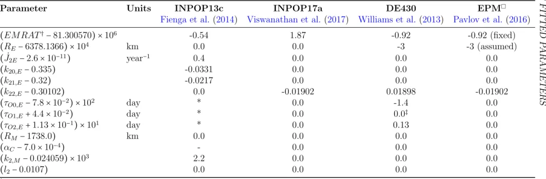
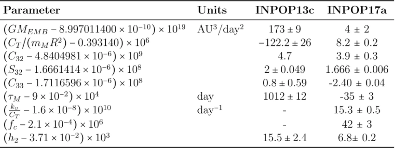
5.2 List of fitted parameters . . . 77

5.2.1 Constraints . . . 80

5.2.2 Correlation . . . 80

5.3 Results . . . 84

5.3.1 INPOP13c vs INPOP17a. . . 84

5.3.2 INPOP17a vs INPOPG . . . 90

5.3.3 INPOP17a vs DE430 and EPM2016 . . . 93

6 Applications 101 6.1 Lunar interior . . . 101

6.1.1 Discussion about INPOP17a model . . . 102

6.1.3 Degree-3 shape of the lunar fluid core . . . 106

6.2 Test of the principle of equivalence . . . 110

6.2.1 Context . . . 110

6.2.2 Method . . . 111

6.2.3 Results . . . 111

6.2.4 Discussion . . . 114

6.2.5 Perspectives . . . 115

7 Conclusion and Perspectives 117 Appendices 121 A Adjustments to reference points 123 A.1 Estimation of coordinates . . . 123

A.1.1 LLR Station coordinates . . . 123

A.1.2 LLR retroreflector coordinates . . . 123

A.2 Station biases . . . 123

B Supplementary materials 127 B.1 Correlation matrix and partial derivatives . . . 127

B.2 Topographic coupling at CMB . . . 135

C Article submitted to A&A: under revision 137

D Article submitted to MNRAS 147

List of Tables

2.1 Comparison of the performance of the Grasse station correlation algorithm and the Expectation Maximization algorithm (EM) using simulated LLR observations and noise, under the cases described in the text (Section 2.2.5). . . 28 5.1 Fixed parameters for the Earth-Moon system. . . 83

5.2 Comparison of extended body parameters of solution: INPOP13c

vs INPOP17a. Fitted parameters are indicated with their corre-sponding formal uncertainties (1-σ) . . . 85 5.3 Comparison of post-fit residuals of LLR observations from ground

stations with corresponding time span, number of normal points available, number of normal points used in each solution after a 3-σ rejection filter. The WRMS (in cm) is obtained with solutions

INPOP13c (1969-2013) and INPOP17a (1969-2017). ‡_{: Statistics}

drawn fromFienga et al. (2014) . . . 89 5.4 Reflector-wise statistics computed using residuals obtained with

INPOPG and INPOP17a, within the fit intervals 01/01/2015 to

01/01/2017 (with a 3-σ filter), with the WRMS in m (RMS weighted by number of observation from each reflector). Refer to Section (5.3.2) for the description of the solutions. . . 92

5.5 Extended body parameters for the Earth and the Moon.

Uncer-tainties for INPOPG and INPOP17a (1-σ) are obtained from a 5%

jackknife (JK). DE430 uncertainties seem to be inflated (unknown scaling) formal uncertainties and EPM solutions provide the 1-σ formal uncertainties. †_{: C}

32, S32 and C33 are reference values from

the GRAIL analysis byKonopliv et al.(2013). ‡_{: h}

2 reference value

from LRO-LOLA analysis by Mazarico et al. (2014). ∗ _{: derived}

quantity. Refer to Section 5.3.2 for the description of the solution INPOPG . . . 96

xii LIST OF TABLES

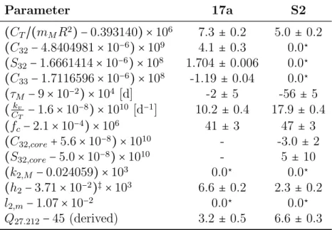
6.1 Comparison between solutions: Extended body parameters for the Moon. Uncertainties are obtained from a 5% jackknife (JK) test, the least squares 1-σ uncertainties being either consistent or smaller than the JK estimations. ⋆_{stands for values fixed to model (GL0660b)}

values from GRAIL. 17a refers to the INPOP17a solution and S2 refers to an internal version of INPOP with the dynamical model described in Section (6.1.3). ‡ _{indicates that the h}

2 reference value

is extracted from Mazarico et al. (2014). . . 108 6.2 Comparison of results for the ratio ∆ESM (Column 4) estimated

with the solution INPOP17A with LLR dataset between: 1) 1969-2011 (for comparison with (Williams et al., 2012b; M¨uller et al.,

2012)); 2) 1969-2017 with data obtain only in Green wavelength, 3) 1969-2017 with data obtained with both Green and IR wavelength. Column 5 contains the converted cos D coefficient expressed in mm (see Eqn. 6.2). Column 6 empirically corrects the radial perturba-tion for effects related to solar radiaperturba-tion pressure and thermal ex-pansion. Column 7 contains the ratio ∆ESM derived from Eqn. 6.2

and values of Column 6.. . . 113 6.3 Results of the SEP estimates obtained from the LLR EP numerical

estimates, after removing the WEP component provided by the lab-oratory experiments from Adelberger (2001);Williams et al. (2009). 114 A.1 Fitted values of LLR station coordinates and velocities (expressed

in meters and meters per year respectively), at J2000.0, for different solutions. The reference values correspond to ITRF2005. ⋆_indicates

fixed parameters. . . 124 A.2 Fitted values of selenocentric coordinates of reflectors (in meters).

The reference values are from a previous release of INPOP (Fienga et al., 2014, p. 27). . . 125 A.3 Estimated values of station biases over different periods (2-way light

List of Figures

1.1 The Earth-Moon system: The angle between the Earth’s equator

and the ecliptic, or the plane of the Earth’s orbit around the Sun, is 23.5 degrees, and this tilt produces the seasons. The Moon provides a steadying influence for the Earth’s tilt, keeping it from varying widely and producing dramatic climate variations. Also note that the plane of the lunar orbit falls neither in the Earth’s orbital plane nor in the ecliptic. Source: Kenneth R Lang (2011, p. 184). . . 3 1.2 According to the fission hypothesis (left), the rotational speed of the

young Earth was great enough for its equatorial bulge to separate from the Earth and become the Moon. In the capture hypothesis (middle), a vagabond Moon-sized object once passed close enough to be captured by the Earth’s gravitational embrace. We have pictured disruptive capture, with subsequent accretion, but the Moon might have been captured intact. The accretion hypothesis (right) asserts that the Moon formed from a disk near the young Earth. Source:

Kenneth R Lang (2011, p. 197) . . . 4 1.3 Massive projectile (A) striking the young, still forming Earth (B)

nearly 4.6 billion years ago. Some of the ejected mass fraction re-mained in Earth orbit (C). A proto-Moon began to form from the orbiting material (D), accreting neighborhood matter, and finally became the Moon (E). Source: Kenneth R Lang (2011, p. 198) . . . 5 2.1 Lunar return pulses over a ranging session at Grasse station using

532 nm laser. File reference: 14121704.09b . . . 14 2.2 Example of calibration profile (measured) from the Grasse station

. µcal = 100.29 ns and σcal = 60 ps (with FWHM ≈ 150 ps). File

reference: 13010303.08b . . . 17 2.3 Fixed shape of a correlation kernal (simulated) used within the

nor-mal point algorithm at the Grasse station, for peak determination of return pulse using the correlation method. Correlation kernal width is chosen so as to match the binning used for the observations. 18

xiv LIST OF FIGURES

2.4 Lunar return pulses over two ranging session at Grasse station using 532 nm laser. Equal number of photon count is detected between multiple binning intervals, due to which the automatic peak detec-tion algorithm fails to resolve the peaks within the histogram. File reference: 14121705.47b (top), 13010402.33b (bottom). . . 19 2.5 Filtered lunar return pulses over a ranging session at the Grasse

station using 532 nm laser. The distribution is clearly asymmetric due to the combined effect of photo-diodes and timing electronics. The reflector orientation would not contribute to this asymmetry, as the array is considered to be uniform. File reference: 15032717.44b 21

2.6 Improvement in normal point sigma by replacing LLR residuals

within the Grasse station full rate data (original), with DE430 ephemeris and GINS reduction model processed residuals (replaced). An improvement of 5% on the standard deviation is noticed. The offset from zero is due to the uncorrected calibration value. . . 22 2.7 Cumulative distribution function of photon count/session obtained

with the 532 nm (Green) wavelength (2014-2017) and the 1064 nm (IR) wavelength (2015-2017) at the Grasse LLR station. . . 33 2.8 Histogram of annual frequency of LLR data from LLR stations (with

the percentage contributions indicated above) with relative contri-bution from each LRR array including Grasse IR (1064 nm) observa-tions. Points indicate the annual mean of post-fit residuals (in cm) obtained with INPOP17a. The dominance of range observations to Apollo reflectors is evident. A change can be noticed after 2014 due to the contribution from IR at Grasse. . . 35 2.9 Grasse reflector wise distribution at 532 nm and 1064 nm from 2015

to 2017. . . 36 2.10 Spatial distribution of retro-reflectors on the lunar surface.. . . 38 2.11 APOLLO and Grasse LLR observations in terms of i) observational

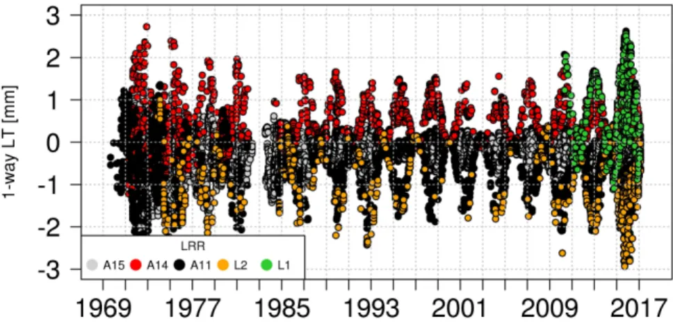
accuracy as given by the annual mean of normal point uncertainty (converted from ps to 1-way light time (LT) in cm) and ii) annual weighted root mean square of post-fit residuals (1-way LT in cm) obtained with INPOP17a. . . 39 2.12 Distribution of IR wavelength LLR observations over 2 years from

Grasse vs lunar phase. . . 40 2.13 Distribution of Green wavelength LLR observations over 2 years

from Grasse vs lunar phase. . . 40 2.14 Distribution of Green wavelength LLR observations over 2 years

3.1 Schematic of the movement of the Earth-Moon system. The light-time computation involves the state vectors (position (P) and veloc-ity (V)) of the Earth and the Moon at a given time (T), in the ICRF reference frame, at: emission of the laser pulse from the station on the Earth, reflection of the laser pulse off the lunar retro-reflectors, and reception of the reflected pulse at the Earth station. . . 45 3.2 θ is the angle of nutation between ⃗K and ⃗k, φ is the angle of

pre-cession between ⃗i and ⃗OΩ, ψ is the rotation angle between ⃗OΩ and ⃗I. Ω is the ascending node. Courtesy: Manche(2011, Fig. 3.1) . . . 49 3.3 Multi-geodetic characterization of the seasonal signal at the Grasse

geodetic reference station, France. Strong correlation between GPS observations and non-tidal loading predicted deformation due to hydrology. LLR observations agree reasonably well with GPS and hydrology loading predictions in the U component. The estimated amplitude of the effect is (8.5 ± 0.5) mm in the Up component. LLR observations lack sensitivity in the other directions and hence are not provided. Grasse observations are stacked and averaged by month over 13 years. Used with permission fromM´emin et al.(2016). 56 5.1 Bias correction and weight scaling requirement for LLR

observa-tions from APOLLO (top) and Grasse (bottom) staobserva-tions. Points in orange and black indicate the post-fit residuals [1-way LT in cm] be-fore and after the correction of estimated bias through LLR analysis. Bias numbering corresponds to that provided in Table (A.3). Points in red indicate the normal point uncertainty from the LLR observa-tion after scaling. Uncertainties from Grasse staobserva-tion are divided by the square root of the number of echoes of each LLR normal point (as recommended), to allow comparison with the uncertainties from the APOLLO station. . . 72

5.2 Unscaled uncertainties of LLR observations from APOLLO (top)

and Grasse (bottom) stations. All the marked regions for APOLLO correspond to logged changes at the station. For Grasse station, regions - A1, A2 and C have unrealistic (near-zero) uncertainties due to suspected rejection filter scaling issues within the normal point algorithm as addressed in Section (2.2.3).. . . 73 5.3 Annual mean of weights from different LLR stations after scaling the

uncertainties present within LLR observation (converted to 1-way LT [cm]). The observations obtained from Grasse during 2010-2017 have an accuracy at nearly the same level as of APOLLO station. . 75

xvi LIST OF FIGURES

5.4 Jackknife (JK) data sampling with 5% of total observations re-moved for variance estimation. The selection is performed from a uniform random distribution (points in red). . . 77 5.5 Comparison of differences in geocentric distance of the Moon (in m)

with DE430 using a) INPOP13c (in black) and b) INPOP17a (in red). The reduction in the radial differences is due to the reduction of the estimated parameter GMEM B, indicating a more consistent

estimate with DE430 (Williams et al., 2013). . . 86 5.6 Comparison of differences in lunar Euler angle rates (where ˙φ: rate

of precession angle, ˙θ: rate of nutation angle and ˙ψ: rate of rotation angle) with DE430 using a) INPOP13c (in black) and b) INPOP17a (in red). . . 87 5.7 Post-fit residuals in (cm) vs time (year) obtained with INPOP17a

for : a) GRASSE station with the 532 nm wavelength, b) GRASSE station with the 1064 nm wavelength, c) McDonald, MLRS1, MLRS2, Haleakala and Matera stations, d) APOLLO station. Post-fit resid-uals here are filtered at 5-σ. . . 98 6.1 Longitude libration signature of ±1 mm over 48 years on the 1-way

light time range (0.33 mas on longitude libration) with a period of about 3 years (weak) arising from the introduction of higher order figure-figure interaction (fourth degree torque) between the Moon and the Earth, as provided by ⃗N22torque inBois et al. (1992, p. 197).104

6.2 Longitude libration signature of ±3 mm over 48 years on the 1-way light time range (1 mas on longitude libration) with a period of about 3 years arising from the introduction of higher order inter figure-figure interaction (fifth degree torque) between the Moon and the Earth, as provided by ⃗N23 torque in Bois et al.(1992, p. 198). . 105

6.3 Contribution of degree-3 love number on the 1-way light time range. 106 6.4 Longitude libration signature arising from unmodeled effects within

the dynamical model, with a period of 6 year and amplitude 5 cm on the range. Post-fit residuals (in 1-way light time [cm]) obtained with APOLLO station data vs time (in years) from solution with : (left) GRAIL-derived degree-3 lunar gravity field coefficients, (cen-ter) LLR-derived degree-3 lunar gravity field coefficients (C3,2, S3,2

and C3,3), (right) GRAIL-derived degree-3 lunar gravity field

coef-ficients with the model described in Section (6.1.3). . . 109 B.1 Correlation between the parameters of the dynamical model and

B.2 Reflector-wise plot of partial derivatives of dynamical model pa-rameters: A15 (Blue), A14 (Green), A11 (Black), L2 (Cyan), L1 (Red). δ indicates the amplitude of the deviation from the central value used for the respective parameter. Label Xc represents the

parameter X with the subscript (c) indicating the lunar fluid core. . 129 B.8 Correlation between core degree-3 spherical harmonics arising from

List of Abbreviations

AIRS Atmospheric Infrared Sounder

APOLLO Apache Point Observatory Lunar Laser-ranging Operation

BCRS Barycentric Celestial Reference System

BVLS Bounded-Value Least-Square

CCD Charge-Coupled Device

CDF Cumulative Distribution Function

CERGA CEntre de Recherches en G´eodynamique et Astrom´etrie

CIO Celestial Intermediate Origin

CIP Celestial Intermediate Pole

CMB Core-Mantle Boundary

CMP Conventional Mean Pole

CNES Centre National d’Etudes Spatiales

CRD Consolidated Range Data

DE Developmental Ephemeris

DGP Dvali-Gabadadze-Porrati theory

EGM Earth Gravitational Model

EM Earth-Moon

EM Expectation Maximization

EOP Earth Orientation Parameter

EOST Ecole et Observatoire des Sciences de la Terre

EP Equivalence Principle

EPM Ephemerides of Planets and the Moon

ESA European Space Agency

FCN Free Core Nutation

FES Finite Element Solution

GCRF Geocentric Celestial Reference Frame

GGM Global Gravity Model

GINS G´eod´esie par Int´egrations Num´eriques Simultan´ees

GLDAS Global Land Data Assimilation System

GPS Global Positioning System

xx LIST OF ABBREVIATIONS

GRACE Gravity Recovery And Climate Experiment

GRAIL Gravity Recovery and Interior Laboratory

GRGS Groupe de Recherche de G´eod´esie Spatiale

GRT General Relativity Theory

GSFC Goddard Space Flight Center

IAA Institute of Applied Astronomy

IAU International Astronomical Union

ICRF International Celestial Reference Frame

IERS International Earth Rotation and Reference Systems

IfE Institut f¨ur Erdmessung

ILRS International Laser Ranging Service

IMCCE Institut de M´ecanique C´eleste et de Calcul des ´Eph´em´erides

INPOP Int´egrateur Plan´etaire de l’Observatoire de Paris

IR Infra-Red

ITRF International Terrestrial Reference Frame

ITRS International Terrestrial Reference System

JD Julian Day

JK Jack-Knife

JPL Jet Propulsion Laboratory

KEOF Kalman Earth Orientation Filter

KREEP potassium (K), rare earth elements (REE), phosphorous (P)

LCRF Lunar-Centric Reference Frame

LLR Lunar Laser Ranging

LOLA Lunar Orbiter Laser Altimeter

LP Lunar Prospector

LPSC Lunar and Planetary Science Conference

LRO Lunar Reconnaissance Orbiter

LRRR Lunar Ranging Retro Reflector

LS Least-Square

LT Light time

MERRA Modern-Era Retrospective analysis for Research and

Applica-tions

MICROSCOPE MICROSatellite `a traˆın´ee Compens´ee pour l’Observation du Principe d’Equivalence

MIT Massachusetts Institute of Technology

MLE Maximum Likelihood Estimation

MLRS McDonald Laser Ranging System

MNRAS Monthly Notices of the Royal Astronomical Society

NASA National Aeronautics and Space Administration

Nd:YAG Neodymium-Doped Yttrium Aluminium Garnet

OCA Observatoire de la Cˆote d’Azur

PA Principal Axis

PDF Probability Distribution Function

PEP Planetary Ephemeris Program

PKT Procellarum KREEP Terrane

POLAC Paris Observatory Lunar Analysis Center

RAS Russian Academy of Sciences

RMS Root Mean Squares

SEP Strong Equivalence Principle

SLR Satellite Laser Ranging

SOFA Standards of Fundamental Astronomy

SSB Solar-System Barycenter

SVD Singular Value Decomposition

TAI Temps Atomique International

TCB Temps Coordonn´ee Barycentrique

TCG Geocentric Coordinate Time

TDB Temps Dynamique Barycentrique

TT Terrestrial Time

UFF Universality of Free Fall

UT Universal Time

UTC Universal Coordinated Time

VLBI Very-Long-Baseline Interferometry

WEP Weak Equivalence Principle

WLS Weighted Least-Square

2 CHAPTER 1. INTRODUCTION

rate of about 2-3 ms per century. One of the fundamental laws of physics is the law of conservation of momentum. A loss in the rotational angular momentum equals the gain in the orbital angular momentum. Hence as the Earth slows down, the momentum lost is transferred to the Moon’s orbit. This gain results in the increase of the distance between the Earth and the Moon, as their masses remain constant. The rate of this outward motion of the Moon amounts to about 3.8 cm/yr. This value is also measurable with the analysis of laser ranging from the Earth (Williams et al.,2014c), to the lunar retro-reflectors placed on the Moon by Apollo astronauts during the Cold War inspired Space Race era.

If this outward motion is extrapolated into the past, we see that the Moon was closer to the Earth, 4.6 billion years ago, when the Earth and Moon were formed. This suggests the formation of the Moon near or even out of the Earth in the distant past, considering stronger tidal interaction propelling the Moon outward at a quicker rate.

1.1.1

Formation and evolution mechanism

How did the Moon form? What theory best explains the origin of the moon? Any theory of the Moon’s origin, must explain, the Moon’s relatively large mass with respect to its planet Earth. Mars is the only other terrestrial planet to have a moon, however its two satellites are relatively very small. The giant planets have extensive satellite systems, but their moons are usually composed of low-density rock-ice mixtures unlike our high-density rocky Moon.

A satisfactory theory must also explain the Moon’s peculiar orbit which lies at 5 degrees to the ecliptic plane (plane of the Earth’s orbit around the Sun) which is itself tilted 23.5 degrees with respect to the Earth’s equatorial plane (see Fig.1.1).

Furthermore, its mean mass density of about 3344 kg/m3

is much lower than the Earth’s mean mass density of 5513 kg/m3_.

Comparison of the lunar rocks returned from the lunar sample return missions provides further constraints on the Moon’s history. The oldest rocks on the Moon solidified about 4.5 billion years ago, which means that the Moon is about as old as the Earth. An important distinction comes from the similar quantities of oxygen isotopes in both Moon and Earth rocks, suggesting common ancestry, instead of the Moon forming elsewhere and then being captured by the Earth’s gravity. Another key constraint is the compositional differences, with Moon rocks lacking any detectable water-bearing minerals, or other kinds of volatile elements with low melting points. Yet when compared to the Earth, the Moon is enriched in non-volatile substances having high melting points that require high temperatures and extraordinary heat to vaporize into space.

Fission, capture and co-accretion models (see Fig. 1.2) of lunar origin have all been studied in great detail for more than a century, but none satisfies both the

6 CHAPTER 1. INTRODUCTION

Observations from the Apollo data hinted that a dichotomy in the geologic processes may have existed between the lunar nearside and far-side. Topographic data obtained from the laser altimeter on the Apollo 15 probe, showed that there was a 2-km displacement between the Moon’s center of mass and center of figure roughly along the Earth-Moon axis (Kaula et al., 1972), suggesting far-side crust was thicker than that of the nearside.

Electromagnetic-sounding data placed an upper limit of about 500 km on the core radius (Hood, 1986). The measurement of a weak, induced dipolar magnetic field as the Moon passes through the Earth’s geomagnetic tail implies the existence of a high-electrical-conductivity core with a radius of about 340 ± 90 km (Hood et al.,1999), whereasShimizu et al.(2013) found a radius of 290 km with an upper bound of 400 km. Additionally, the analyses of small rotational signatures obtained from the lunar laser ranging experiment indicate that the energy is currently being

dissipated at the boundary between a molten core and a solid mantle (Williams

et al., 2001), providing an upper limit of 374 km for a Fe-FeS eutectic fluid core and a 352 km upper limit for a pure Fe composition.

While the available evidence indicates that the Moon possess a small molten core, the geophysical data could not unambiguously constrain its composition as none of the well-determined seismic ray paths, collected by the small network of lunar seismometers, pass through the deepest portion of the lunar interior ( Wiec-zorek, 2009).

Reanalysis of the Apollo-era seismic data using array-processing methods sug-gests the presence of a solid inner and fluid outer core, with a partially molten boundary layer (Weber et al., 2011). However, analysis by another group Gar-cia et al. (2011), reports the remaining inconsistencies within Weber et al. (2011) and concludes with a lunar model without a solid inner core due to the strong uncertainties of the different parameters used.

Many of the samples returned contained high concentration of KREEP

(potas-sium (K), rare earth elements (REE) and phosphorous (P)). Lawrence (1998)

provides the surface thorium concentrations obtained from the Lunar Prospec-tor gamma-ray spectrometer, showing high concentration of heat sources on the nearside region called Procellarum KREEP Terrane (PKT). A more recent study byLaneuville et al.(2013), show with the help of thermo-chemical convection mod-els, that the impact of such localized heat sources in the crust leaves a present-day temperature anomaly within the nearside mantle with its influence down to the core-mantle boundary (CMB).

Contributions from GRAIL and LLR

The gravity field of a planet provides a view of its interior and thermal history by revealing areas of different density. The Gravity Recovery and Interior Laboratory

(GRAIL) mission placed a pair of satellites in an orbit around the Moon, acting as a highly sensitive gravimeter, and began mapping the Moon’s gravity in early 2012. Zuber et al. (2013) provide the lunar gravity field to spherical harmonic degree and order 420, obtained from the spacecraft-to-spacecraft tracking observations from the GRAIL mission. The study revealed several new tectonic and geologic features of the Moon. Impacts have worked to homogenize the density structure of the Moon’s upper crust while fracturing it extensively. Wieczorek et al.(2013) show that the upper crust is 35 to 40 kilometers thick and less dense and thus more porous than previously thought. Andrews-Hanna et al.(2013) show that the crust is cut by widespread magmatic dikes that may reflect a period of expansion early in the Moon’s history.

From the 3 months of data collected over the primary mission, two independent groups at the Jet Propulsion Laboratory (JPL) and Goddard Space Flight Center (GSFC) determined the lunar gravity field (Konopliv et al., 2013; Lemoine et al.,

2013) up to degree and order 660, with comparable estimates and uncertainties

between the groups.

While the high-degree coefficients are very well determined, the solutions for the low-degree coefficients are very sensitive to the libration model (obtained from the fit of lunar ephemerides to lunar laser ranging (LLR) data) and to the models of the non-gravitational acceleration on the GRAIL spacecraft including the empirical periodic acceleration model (Konopliv et al., 2013). The physical libration model of the Moon from Williams et al.(2013) consists of a solid crust and mantle plus a uniform fluid core, without a solid inner core. Williams et al. (2014b) introduced variations on the models of Weber et al. (2011) andGarcia et al. (2011) to satisfy the lunar mean density, mean solid moment of inertia, love number and a deep low-velocity zone constraints to account for a solid inner core surrounded by an outer fluid core (see Williams et al. (2014b, Table 7-8)) to give a family of lunar interior models.

A detection of the solid inner core is feasible from very precise measurements of the lunar gravity field. The axis of rotation of a solid inner core within a liquid outer core can be different from the axis of the mantle. With an axis of rotation tilted by a different amount than the mantle, the inner core degree-2 spherical harmonics would produce variable gravity field as the core rotates. This causes a time varying C21 and S21 harmonics (when viewed in a mantle-fixed frame) with

a period of 27.212 days (Williams, 2007). The search for variable C21 and S21

harmonics was one of the goals of the GRAIL mission. Though the mission goals were met, the search for the inner core periodicities did not find results above the noise level (Williams and Watkins, 2015). The detection of the solid inner core would provide further constraints to the models of lunar origin and evolution and answer key questions related to the possible existence of a now-extinct lunar

8 CHAPTER 1. INTRODUCTION

dynamo (Wieczorek, 2006; Laneuville et al.,2014).

Combining gravity field with other observational techniques provides synergis-tic advantage to the problem. Laser-altimeter data from a lunar orbiting spacecraft (e.g. LRO-LOLA) provides constraints on the body tides (Mazarico et al., 2014) and LLR provides rotational signatures (Rambaux and Williams, 2011). A study that combines these constraints (Matsuyama et al.,2016) provide probability dis-tribution curves to the lunar solid inner core size and liquid core density. This can then be used to provide constraints on the thermal evolution of the lunar core and hence providing a link to its evolution. However,Matsuyama et al.(2016) did not consider the hemispheric asymmetry found byLaneuville et al. (2013);Zhang et al. (2013), which could influence the estimates of the lunar interior structure due to the tidal forcing brought by the asymmetry (Qin, 2015).

Thermal evolution models suggest that a portion of the core should have crys-tallized to form a solid inner core at its center (Zhang et al., 2013; Laneuville et al., 2013; Scheinberg et al., 2015). Hence, similar to the gravitational torques of the Earth acting on the lunar mantle, the Earth should also drive a tilt of the elliptical figure of the solid inner core, forcing it to precess with the 18.6 year

period lunar mantle precession (Dumberry and Wieczorek, 2016). Furthermore,

the gravitational torques exerted by the inner core on the lunar mantle may affect the Cassini state of the lunar mantle, similar to that expected for Mercury (Peale et al.,2016). This would in turn be detectable by LLR, provided the accuracy and time span of the LLR observations permit.

LLR observations continue to bring critical information in terms of libration sensitive low-degree gravity field coefficients due to its long time span and high ac-curacy, which would complement the low-degree coefficients of the GRAIL-derived gravity field models for the detection of the solid inner core of the Moon.

1.2

Tests of general relativity

The year 2015 marked the 100th anniversary of General Relativity Theory (GRT) (Einstein,2015). Up to now, GRT successfully described all available observations and no clear observational evidence against General Relativity was identified. How-ever, the discovery of Dark Energy that challenges GRT as a complete model for the macroscopic universe and the continuing failure to merge GRT and quantum physics indicate that new physical ideas should be searched for. To streamline this search it is indispensable to test GRT in all accessible regimes and to highest possible accuracy.

Violations of the Equivalence Principle (EP) are predicted by a number of modifications of GRT aimed to suggest a solution for the problem of Dark

Damour and Donoghue,2010;Damour,2012). The Universality of Free Fall (UFF), an important part of the Equivalence Principle, is currently tested at a level of about 10−13 _{with torsion balances (Adelberger et al.,2003) and the LLR (Williams}

et al., 2012a; M¨uller et al., 2012). EP violations and time variations in the fun-damental coupling constants could also be a result of the effects of a scalar field coupling with the gravitational field (Damour, 1996; Damour and Vokrouhlick´y, 1996). Therefore, tests of EP and ˙G have great importance due to its wide reach as sensitive probes towards new physics (Murphy, 2013).

Some other formalisms often used to test gravity in the solar system and to solve some questions raised by the Dark Matter and the expending universe can also be tested with the LLR measurements: the modification of the inverse square law of gravity (Falcon, 2011), additional force represented by Yukawa-type expression (Adelberger et al.,2003;M¨uller et al., 2005).

“Measurement of the precession rate can also probe a recent idea (called Dvali, Gabadadze, Porrati (DGP) gravity) in which the accelerated expansion of the universe arises not from a non-zero cosmological con-stant but rather from a long-range modification of the gravitational coupling, brought about by higher-dimensional effects (Lue and Stark-man, 2003; Dvali et al., 2003; Dvali et al., 2003). Even though the lunar orbit is far smaller than the Gigaparsec length-scale characteris-tic of the anomalous coupling, there would be a measurable signature of this new physics, manifesting itself as an anomalous precession rate at about 5 µarcsec.yr−1_{, roughly a factor of 10 below current LLR}

lim-its, and potentially reachable by millimeter quality LLR.” – (Murphy, 2013, p. 8)

Tests of GRT remains as an important tool to streamline the theoretical de-velopment. While a number of space missions are planned to improve these tests (MICROSCOPE to test the UFF with the level of 10−15 _{(Berg´e et al., 2015), Gaia}

(Hees et al.,2015) and BepiColombo (de Marchi and Congedo,2017) to provide a number of high accuracy tests of GRT, EUCLID (Laureijs et al.,2011) to study the distribution of Dark Matter in our Galaxy and the Universe, etc.), the instrumen-tation proposed here will lead to study the solar system dynamics for aiming at a set of advanced GRT tests that are complementary to the planned space-mission tests.

Finally, direct measurement of Dark matter in the solar system is also proposed by Nordtvedt et al. (1995) with the detection of its gravitational influence on the most accurately measured quantity in the solar system, the Earth-Moon distances (Merkowitz, 2010).

10 CHAPTER 1. INTRODUCTION

1.3

Ephemerides and its applications

The 1960’s were a turning point for the generation of ephemerides, before which analytical models were used for describing the state of the solar system bodies

as a function of time. A team from the Lincoln Laboratory, MIT (Ash, 1965)

introduced the planetary ephemeris program (PEP) on a computer software using FORTRAN IV language, to improve the planetary and lunar ephemerides using the results of radar and optical observations. The first laser ranges to the lunar retro-reflectors were obtained in 1969 after the Apollo landing (Faller et al.,1969). The change from lunar angular measurements to laser ranges marked a great im-provement to the observational accuracy driving comparable imim-provements to the lunar ephemerides (Bender et al., 1973). Opportunities to test the theory of gen-eral relativity also surfaced (Shapiro,1964;Nordtvedt,1968;Williams et al.,1976; Anderson et al., 1978).

While the fitting of optical data was long accomplished with analytical the-ories for the Moon and planets, the improved data required the development of numerical integration techniques and more comprehensive physical models. In the late 1970’s the numerically integrated planetary ephemerides were built by the Jet Propulsion Laboratory (JPL), called the developmental ephemeris (DE96) (Standish et al., 1976). Since then, there have been many versions of the JPL DE ephemerides through the present (Newhall et al.,1983;Standish Jr,1990;Standish, 1998,2006; Folkner et al.,2009; Folkner et al., 2014). These ephemerides are con-tinuously fitted to the data gathered from tracking space probes (radar ranging, flybys and VLBI), optical data (transit, photographic plates and CCD observa-tions for outer planets) and direct range measurements (LLR). Semi-analytical

theories also emerged to take advantage from both the worlds (Chapront-Touze

and Chapront,1983), however they lack accuracy when compared with numerically integrated ephemerides.

Simultaneously, with the growing interest in space sciences, the European Space Agency (ESA) was actively involved in interplanetary missions and col-laborated with other national space administrations. With these developments, the “Int´egrateur Plan´etaire de l’Observatoire de Paris” (INPOP) project was ini-tiated in 2003 to build the first European planetary ephemeris independently from JPL. The INPOP project evolved over the years with the first official release in 2008: INPOP06 (Fienga et al., 2008) followed by versions 08-15 (Fienga et al., 2009; Fienga et al., 2011; Fienga et al., 2014, 2015, 2016a). Through the official website2 _{of the“Institut de M´ecanique C´eleste et de Calcul des ´Eph´em´erides”}

(IM-CCE), these ephemerides are freely distributed to the users. With the help of ephemerides, the users can have access to the positions and the velocities of the

2

major planets, Moon and asteroids of our solar system, the libration angles of the Moon as well as the differences between the terrestrial time TT (time scale used to date the observations) and the solar system barycentric times (TDB/TCB) (time scales used in the equations of motion). The ephemerides can be accessed using CALCEPH (Gastineau et al.,2015) or SPICE (Acton, 1996) toolkit libraries.

In addition to INPOP and DE, another numerical ephemeris are those devel-oped by the teams at the Institute of Applied Astronomy (IAA) of the Russian Academy of Sciences (RAS), called the Ephemerides of Planets and the Moon (EPM) (Pitjeva,2005,2013). These ephemerides are based on the same modeling

as the JPL DE ephemerides. The most recent version being EPM2016 (Pavlov

et al., 2016).

As numerical ephemerides are fitted to real observations, the mathematical model backing the ephemerides follow closely with the real-world processes. This enables a more realistic simulation of the natural processes allowing comparison of the real observations with simulated observations. Any remaining differences (post-fit residuals) between the simulated and the real observations indicate un-modeled effects within the numerical model provided the amplitude of the differ-ences are greater than the level of the known accuracy of the real observations and also considering the absence of modeling errors at the same level. Introducing model additions/changes based on the detected unmodeled effects continuously improve the quality of the simulation as well as provide best-fit estimates of the model parameters.

Traditionally, numerical ephemerides are used to satisfy high accuracy require-ments for spacecraft navigation and mission planning. Other scientific applications include (but are not limited to) orbit determination and localization (Fienga et al., 2016a), reference frame ties (Folkner et al.,1994), gravity field determination (Iess et al., 2014; Folkner et al., 2017) asteroid mass determination (Kuchynka et al., 2010), fundamental physics (Bertotti et al., 2003; Williams et al., 2004; Fienga et al., 2011; Fienga et al., 2016b), solar corona studies (Verma et al., 2013) and paleoclimate studies (Laskar et al., 2004, 2011).

For this study, we develop on the INPOP planetary and lunar ephemeris, as a laboratory to perform tests relevant to two of the interests described in the previous sections: lunar interior structure (Section 1.1) and test of the violation of the universality of free fall using the principle of equivalence (Section 1.2), in using LLR observations and a GRAIL-derived gravity field model (Konopliv et al., 2013).

12 CHAPTER 1. INTRODUCTION

1.4

Outline of the thesis

The following describes a brief outline of this thesis:

Chapter (2) discusses the observations used for this study, consisting of lunar laser ranging (LLR) data acquired between 1969 to 2017 from various LLR stations. The existing normal point algorithm at the Grasse LLR station is evaluated and an alternative algorithm is proposed. New LLR observations from the Grasse station obtained using the IR (1064 nm) wavelength are also included and its benefits are discussed.

The numerical model for the Earth-Moon system consists of two components: the reduction model (Chapter3) and the dynamical model (Chapter 4). The geo-physical and relativistic effects implemented within the reduction model (GINS software) are discussed with its impact on the Earth-Moon distance. The dynam-ical model consists of the INPOP planetary and lunar ephemeris. The lunar part of the ephemeris is described with the improvement from the previous model (IN-POP13c).

Chapter (5) describes the processes behind the construction of a lunar ephemeris followed by the analysis of the post-fit residuals and comparison of the model pa-rameter estimates with previous LLR analyses. A technical report on the new INPOP solution (INPOP17a) is published within the “Notes Scientifiques et Tech-niques de l’Institut de M´ecanique C´eleste”, Viswanathan et al. (2017).

Chapter (6) applies the results to the study of lunar interior structure and a strong longitude libration signature of 6 years is detected. Investigation attempts to correct this signature are discussed and a model is provided. An article on the study of the lunar interior structure is submitted to the Astronomy & Astrophysics journal provided in Appendix (C). Chapter (6) also describes a test of the theory of general relativity with respect to the universality of free fall in the Earth-Moon system. A discussion on the results obtained is provided. An article on this work is accepted to the Monthly Notices of the Royal Astronomical Society (MNRAS) and provided in Appendix (D).

Chapter (7) summaries the achieved goals of this thesis, followed by the con-clusion and future perspectives.

Chapter 2

Observation: Lunar Laser

Ranging

2.1

Introduction

Lunar Ranging Retro Reflector (LRRR) arrays were part of the scientific payloads on the three US Manned (APOLLO XI, XIV, XV) and on-board two Soviet Rover (Lunakhod 1, 2) Lunar missions (hereby referred to as A11, A14, A15, L1 and L2 respectively). These arrays were installed by each respective mission, resulting in five distinct positions on the near-side of the Moon.

Ground-based telescopes were used to precisely point to the array location on the lunar near-side, and high energy laser pulses were fired. Initial attempts to ac-quire the return pulses were made at the Lick Observatory in California, US (Faller et al.,1969) with an outgoing beam, approximately 2 seconds of arc, corresponding to a spot diameter of 3.2 km on the lunar surface. Over the next decades, other ground-based telescopes from various sites joined the list of lunar laser ranging

stations, namely, McDonald (Texas) (Bender et al., 1973), MLRS1 and MLRS2

(Texas) (Shelus, 1985), Haleakala (Hawaii) (Berg et al., 1978), Grasse (France) (Veillet et al., 1993; Samain et al., 1998; Torre, 2013), Matera (Italy) (Varghese et al., 1993) and APOLLO (New Mexico) (Murphy et al., 2008). The accuracy of observations improved over time with improvements in detector electronics, aided by larger ground-based telescopes, and improved normal point computation algo-rithms. The most accurate observations are provided by APOLLO station with a 3.5 m telescope (Murphy et al., 2012; Murphy, 2013) and to some extent the Grasse station with recently improved detection capabilities in infrared wavelength (Courde et al., 2017).

Retro-reflectors have the ability to reflect waves in the same direction as the incident waves, arising from the arrangement of the optical mirrors as a corner

2.2

Normal Point

2.2.1

Introduction

A normal point is a reduced observation containing the round trip time of the light pulse at a given time from the spatial reference of the Lunar Laser Ranging (LLR) station on the Earth to the retro-reflector array on the surface of the Moon, computed from many individual echoes. A normal point is computed from full-rate data. The idea is to reduce the data collected from one ranging session (consisting of several echoes) to one single time delay value, the 2-way light time at some specific epoch.

The primary advantage of using a normal point over the full-rate data is the re-duction of the computational complexity achieved through a reduced data volume. Unlike satellite laser ranging (SLR) where the motion of the artificial satellite is rapid within each ranging session, high frequency variations (of a few hundred Hz) within lunar laser ranging are mostly associated with turbulent fluctuations within the Earth’s upper atmosphere and local pressure-temperature gradients. Using a single normal point to represent the full-rate LLR data averages out most of these variations over the 10 minute ranging session. A study on the processes involved for the identification, filtering and reduction of the full-rate LLR data from the McDonald LLR station can be found in Abbot et al. (1973).

In order that the normal point well represents the full-rate data, the algorithm used for the computation of the former must well characterize the distribution of the latter.

In the case of laser ranging to the lunar retro-reflector arrays from ground-based stations, the mean of the detection time distribution comprising of the accumu-lated return pulses, indicates the average difference between the predicted and observed round-trip time taken by the photon. The photons traverse the sum of the total calibration path of the set-up and twice the Earth-Moon distance (up-leg and down-leg). The standard deviation of the detection time distribution is pri-marily due to the contributions from the orientation of the retro-reflector array or target and the response function of the detector and timing electronics, while the shape of the laser pulse fired defines the theoretical minimum (with contributions from the detector and timing electronics). The contribution from the atmospheric turbulences become dominant at low elevation angles (around 10○_{) while LLR is}

typically performed at higher elevation angles (30○ _{to 40}○_{) (Currie and Prochazka,}

2014).

The International Laser Ranging Service (ILRS) Herstmonceux Normal Point algorithm (Pearlman et al., 2002) recommends a tight rejection limit of 2.5-σ for first photo-electron detection systems. This is because such detection systems often involve a photo-diode which is highly sensitive to the first-photon that arrives to

16 CHAPTER 2. OBSERVATION: LUNAR LASER RANGING

the detector. This arrival triggers an avalanche multiplication phenomenon which causes the signature of the detector to influence the skew of the expected return pulse distribution. A scheme for the normal point generation and first-photo bias

at the APOLLO LLR station can be found in Michelsen (2010).

2.2.2

Data format

The historical LLR data spanning over 1969-2016 from all stations is available

pub-licly in the “MINI” format at http://polac.obspm.fr/llrdatae.html. Recent

LLR observations (both in Green and IR wavelength) from Grasse station

(2015-2017) is made available athttp://www.geoazur.fr/astrogeo/?href=observations/

donnees/lune/brutes.

Each LLR normal point contains information about the ground station (ITRF code), targets (lunar reflectors), time of flight of photons (s), observation epoch (UTC), meteorological measurements at the ground station such as atmospheric

pressure (0.01 mbar), ground temperature (0.1 ○_{C) and relative humidity (%),}

wavelength of the laser used (0.1 nm) and data quality information through the number of echoes received, signal to noise ratio and the estimated uncertainties (0.1 ps).

This study uses the MINI format for the normal points. Another format avail-able is the Consolidated Range Data (CRD) useful for kilohertz ranging applica-tions, whose description can be found at the ILRS website1_.

2.2.3

Existing algorithm at Grasse station

The original code employed at the Grasse station uses a Visual Basic program allowing a user interface for the control of laser pulse firing, telescope pointing adjustments and normal point computation based on the Herstmonceux Normal Point Recommendation (Pearlman et al., 2002).

At the Grasse ILRS station, a fixed temporal detection window of±50 ns is used for acquiring the incoming reflected photons after laser firing to the retro-reflectors. The arrival times of the reflected photons are compared with a semi-analytical lunar ephemeris provided by the Paris Observatory Lunar Analysis Center (PO-LAC), accurate to a few centimeters on the lunar orbit2_{. These differences are}

then stacked in time to form an histogram as shown in Fig. (2.1).

This is followed by the determination of the peak of the accumulated return pulses, identified using a correlation method. The accumulated return pulses are correlated with a fixed laser pulse shape. The histogram (Fig. 2.3) is intended to

1

Available at https://ilrs.cddis.eosdis.nasa.gov/data_and_products/formats/crd. html

2

20 CHAPTER 2. OBSERVATION: LUNAR LASER RANGING

tainty computation, the public distribution of the normal points from such instances, impact the regression procedures used by LLR analyses groups (see Section5.1.2).

As a better practice it is recommended by this study to remove such obser-vations from the distributed list of normal points.

• Rejection filter scaling

The ILRS recommends a scaling factor of 2.5 for the rejection filter with systems that detect the first photo-electron. A change in the rejection filter will directly impact the standard deviation of the filtered residuals (and therefore the construction of lunar ephemerides as shown in Section 5.1.2) stored in the normal point, especially when outliers are involved.

Within different versions of the original code available through internal repos-itories at the Grasse station, variations of this scaling factor is noticed from 2.2 to 2.5 prior to year 2000. Such changes made at the Grasse station are often internal and the information is not logged for public access.

As a result, one can notice scaling factors being applied independently by LLR analyses groups (Manche, 2011; Williams et al., 2014a; Pavlov et al.,

2016) while weighting observations during regression, using normal point

uncertainties (see Fig. 5.1.2).

As a better practice it is recommended by this study to:

1. Log changes to algorithm through a publicly accessible domain;

2. Suggested use of a version control tool for all codes impacting publicly released data.

• Fixed shape of correlator

The Grasse station algorithm uses a fixed shape (see Fig. 2.3) within the correlation method for separating the return pulse distribution from accu-mulated noise within the histogram. While this fixed shape approximates to an ideal laser pulse, return pulse distribution from LLR involves other depen-dencies such as that from photo-diodes, timing electronics and retro-reflector orientation (Michelsen, 2010).

Although the current LLR photon detection rate (typically below 100 pho-tons over 10 minutes ranging session) at the Grasse station is not sufficient to fully characterize lunar reflector orientation signatures (trapezoidal), the detected photon distributions are seldom symmetric (see Fig. 2.5). Hence, employing a fixed symmetric Gaussian distribution is only an approximation to the expected pulse distribution. An alternative is to use the calibration profile of the laser pulse at the Grasse station (see Fig. 2.2) obtained by

2006-2012 (Bouquillon et al., 2013), while those from DE430 give about 2 cm (Folkner et al., 2014). The resulting residuals obtained with DE430 is converted to 2-way light time and compared with that obtained with the original predictions present within the LLR full rate data. As one can notice on Fig. (2.6), a 5% improvement of the residual dispersion (σ) is noticed on the replaced light-times due to the accuracy of the underlying ephemeris and improved reduction software, used for the prediction.

This study recommends the use of an updated numerical planetary and lunar ephemerides as the prediction model for LLR observations to obtain a tighter spread of LLR residuals during the normal point computation.

2.2.4

Alternate algorithm

Improvements to the normal point algorithm must be effective to remove unwanted signatures within the full rate data. These may include biases introduced by the detection electronics or from the asymmetry of the projection of the ranging object to the plane wave of laser light. Michelsen(2010) shows the impact of such effects

on normal point algorithm for APOLLO LLR data and Kucharski et al. (2015)

proposes methods to remove satellite (Ajisai) signatures in high-repetition rate (few kHz) SLR normal points for millimeter-level applications in geodesy.

For LLR, although the retro-reflectors are aligned to nominally face the earth center at zero libration (variation in the apparent orientation of the Moon), for any given observation, the reflectors are tilted with respect to the plane wave of laser light. This tilt spreads out the return pulse over the time it takes the wave front to pass from the nearest point on the retro-reflector to the farthest. This has a direct impact on the spread of the core of the Gaussian distribution present in the histogram of the residuals. In addition, the characteristics of the background noise (zero mean or non-zero mean) can cause the histogram to skew towards the mean of the noise. Hence it becomes important to completely characterize the components present in this LLR dataset, rightly called as a mixture model.

In this method of normal point calculation we used the Expectation Maximiza-tion Approach (Gupta and Chen, 2011) in order to decipher the characteristics of the skewed normal components present in the LLR return pulses with back-ground noise, and thereafter computed the normal point for the corresponding LLR dataset.

A Python implementation4 _{is used for the Mixture Model Fitting and adapted}

to a three-component mixture sample (returns from IR and/or Green wavelengths and background noise). The Expectation Maximization (EM) algorithm is imple-mented, for estimating the maximum likelihood of the model parameters (mean

4

24 CHAPTER 2. OBSERVATION: LUNAR LASER RANGING

and variance). In addition we also include the skewness estimate by combining

another Python implementation5

based on the study by Azzalini and Capitanio

(1999) for the generation of skewed normal distribution in the maximum likelihood step.

We assume that the mixture model consists of the linear combination of three Gaussian distributions corresponding to the residuals for Green and/or Infrared lasers, along with the background noise (with the sigma of the background noise chosen to be very large when compared to the residuals to represent a near uni-form noise). The EM method allows to fit a statistical model in the case where the experimental data has unknown variables. These variables provided us the information about which component has generated each sample in our dataset.

With the EM method, we first assigned each sample to each component of the distribution. After which, we computed MLE estimators of parameters of each component of the mixture. Apart from the mean and variance estimates we also introduced a skewness parameter for our study. For each sample si we have three

coefficients γ(i, 1), γ (i, 2) and γ (i, 3) that represent the fraction of si that belong

to the respective components green, IR or noise. And,

γ(i, 1) + γ (i, 2) + γ (i, 3) = 1 (2.1)

where γ is the responsibility function.

The probability distribution function (PDF) f corresponding to the compo-nents in the mixture model follow a Gaussian distribution given by:

f(x∣p) = 1

σ√2πe

−(x−µ) 2

2σ2 (2.2)

The PDF of the mixture becomes: f(x∣p) =

3

∑

k=1

πkfk(x∣p) (2.3)

If we know the parameters p (from our initial guess), we can compute for each sample and each component the responsibility function defined as:

γ(i, k) = πkfk(si∣p) f(si∣p)

(2.4) where, πk is the probability that the sample belongs to the distribution k described

by: πk= Nk N (2.5) 5 Available athttp://azzalini.stat.unipd.it/SN/skew_normal-py.zip

and starting from the effective number of samples for each category (Nk) we

can compute the new estimation of parameters: Nk= N ∑ i=1 γ(i, k) (2.6) where, k= 1, 2, 3 N1+ N2+ N3= N (2.7)

The new mean corresponding to the component k is computed as: µnewk = 1 Nk N ∑ i=1 γ(i, k) ⋅ si (2.8)

Followed by the new variance corresponding to the component k is computed as: σ_k2 new= 1 Nk N ∑ i=1 γ(i, k) ⋅ (si− µnewk ) 2 (2.9) And the new values of skew are computed as:

ξ_knew= 1 Nk N ∑ i₌₁ γ(i, k) ⋅⎛ ⎝ 4− π 2 ⋅ E{X}3 var{X}32 ⎞ ⎠ (2.10) where, δ=√ α 1+ α2 (2.11) E{X} = √ 2 πδ (2.12) var{X} = 1 −2δ 2 π (2.13)

where, α is the shape parameter, which regulates the shape of the density function of the skewed normal distribution.

The skewness is introduced into the Eqn. (2.2) through the shape parameter α with the help of the complementary gauss error function (erfc), as:

fnew(x∣p) = e−(x−µ) 2 2σ2 erf c(−α(x−µ) σ√2 ) σ√2π (2.14)

The following steps are iterated until the convergence criteria is achieved: 1. Recomputation of γ(i, k);