HAL Id: hal-02085261
https://hal.archives-ouvertes.fr/hal-02085261
Submitted on 30 Mar 2019
HAL is a multi-disciplinary open access
archive for the deposit and dissemination of
sci-entific research documents, whether they are
pub-lished or not. The documents may come from
teaching and research institutions in France or
abroad, or from public or private research centers.
L’archive ouverte pluridisciplinaire HAL, est
destinée au dépôt et à la diffusion de documents
scientifiques de niveau recherche, publiés ou non,
émanant des établissements d’enseignement et de
recherche français ou étrangers, des laboratoires
publics ou privés.
Degree-based Outliers Detection within IP Traffic
Modelled as a Link Stream
Audrey Wilmet, Tiphaine Viard, Matthieu Latapy, Robin Lamarche-Perrin
To cite this version:
Audrey Wilmet, Tiphaine Viard, Matthieu Latapy, Robin Lamarche-Perrin. Degree-based Outliers
Detection within IP Traffic Modelled as a Link Stream. 2018 Network Traffic Measurement and
Analysis Conference (TMA), Jun 2018, Vienna, Austria. pp.1-8, �10.23919/TMA.2018.8506575�.
�hal-02085261�
Degree-based Outliers Detection within IP Traffic
Modelled as a Link Stream
Audrey Wilmet
∗, Tiphaine Viard
∗, Matthieu Latapy
∗, Robin Lamarche-Perrin
†∗Sorbonne Universit´e, CNRS, Laboratoire d’Informatique de Paris 6, LIP6, F-75005 Paris, France
†Institut des Syst`emes Complexes de Paris ˆIle-de-France, ISC-PIF, UPS 3611, Paris, France
Email: [email protected]
Abstract—Precise detection and identification of anomalous events in IP traffic are crucial in many applications. This paper intends to address this task by adopting the link stream formalism which properly captures temporal and structural features of the data. Within this framework we focus on finding anomalous behaviours with the degree of IP addresses over time. Due to diversity in IP profiles, this feature is typically distributed heterogeneously, preventing us to find anomalies. To deal with this challenge, we design a method to detect outliers as well as precisely identify their cause in a sequence of similar heterogeneous distributions. We apply it to a MAWI capture of IP traffic and we show that it succeeds at detecting relevant patterns in terms of anomalous network activity.
I. INTRODUCTION
Temporal and structural features of IP traffic are and have been for several years the subject of multiple studies in various fields. A significant part of this research is devoted to detecting statistically anomalous traffic subsets referred to as anomalies, events or outliers. Their detection is particularly important since, in addition to a better understanding of IP traffic characteristics, it could prevent attacks against on-line services, networks and information systems. Methods used in this branch are very broad and depend on both the way in which IP traffic data is modelled and in the statistical analysis used.
Most previous works focus either on the temporal [3], [4] or structural features of traffic [17], [27], with few attempts to combine them [12], [2]. In this paper, we model IP traffic as a link stream which fully captures the both temporal and structural nature of traffic [18], [25]. More specifically, a link stream L is defined as a set of instants T , a set of nodes V (IP addresses) and a set of interaction E (communication between IP addresses over time). Within this framework, we focus on one key property: the degree of nodes. We show that this feature is highly heterogeneous, which raises challenges for its use in outlier detection, but it is stable over time. Our method takes advantage of this temporal homogeneity: it divides the link stream into time slices and then performs outlier detection to find time slices which exhibit unusual number of nodes having a degree within specific degree classes. Then, in order to isolate responsible IP addresses and instants on which they behave unexpectedly, we design an identification method based on an iterative removal of previously detected events. Finally, we validate our method by showing that these events removals do not significantly alter the underlying normal traffic.
The paper is organised as follows. First, we overview the related work in Section II. We introduce IP traffic modelling as a link stream and the degree notion in Section III. In Section IV, we describe our goals and the challenges they raise. This leads to the development of our method to detect events in Section V and to identify them in Section VI. Finally, we discuss our results and conclude in Section VII.
II. RELATEDWORK
Techniques of anomaly detection in IP traffic are extremely diverse. Among those, methods using principal component analysis [16], [22], machine learning [26], data mining [19], signal analysis and graph-based techniques have been
proposed. Concerning signal analysis and graph-based
techniques, an important difference lies in data modelling. On one hand, anomaly detection using signal analysis consists in modelling the data as a temporal signal and then spotting anomalies in the Fourier domain at characteristic frequencies. Even if this approach gives powerful results, some structural aspects of the data are lost [3], [4]. The graph approach on the other hand consists in choosing an observation window of a given size and aggregating the links and nodes appearing during this period to form a static graph. The evolution and the structure of exchanges are then observed and studied via a sequence of static graphs obtained either by translation of the observation window or by aggregation on consecutive windows [17], [27]. Thus, it is assumed that all interactions over the same period of time are comparable, which destroys many temporal aspects. Iliofotou et al. [12] use this representation. They introduce several metrics to study similarities between structural features of two consecutive snapshots. They are able to detect changes of behaviours but not specific sub-graphs. Asai et al. [2] use a different graph approach. They include the temporal information directly into the graph: a node is an interaction and two nodes are linked together if they have a causal relationship. In this way, authors manage to detect abnormal temporal and structural sequences. However, this method is limited by the definition of causal relationships that can not take into account all interactions’properties.
A strength of our work is to preserve both temporal and structural aspects by using the link stream formalism [18], more suited to the data coming from IP traffic. Besides data
modelling, much work has been devoted to the study of anomalies as deviations of the overall traffic volume, like for instance the number of exchanged packets or bytes during a certain amount of time [3], [15]. Link stream formalism allows on the contrary to use more sophisticated features combining both time and structure [18], [25]. The degree for example quantifies the neighbourhood of each node at each moment. Hence, in addition to large events that disrupt traffic volume like flash crowd or alpha flows attacks, it would enable us to detect more subtle and more structurally complex anomalies.
A significant part of our work in this paper is devoted to finding outliers in the degree distribution which is heterogeneous. Up to our knowledge, there is no work dealing exclusively with outliers detection in heterogeneous distributions. Nevertheless, many papers study dissimilarities between different distributions in a way similar to what we do in this paper. Anceaume et al. [1] and Tajer et al. [24] summarize data streams into sketches and apply a distance metric to quantify the similarity between two sketches. Here again, the data used is aggregated and there is a loss of information. Schieber et al. [23] quantify topological difference between two graphs through Jensen-Shannon divergence and a measure of the heterogeneity of each graphs in terms of connectivity distance between nodes. In both cases, methods used only give a similarity score between two different distributions. Our method, besides quantifying a dissimilarity, gives us additional information: where is the dissimilarity located within the distribution, which then makes it possible to identify its origin. Other studies point to this direction, La Fond et al. [14] propose various measurements allowing the comparison of distributions from one time step to the next, but only recover anomalous time slices. Harshaw et al. [10] achieve to find anomalous IP addresses and time slices in series of graphs by comparing, for each graph, the count of specific sub-graphs describing their topology. However, they are still subject to information loss coming from data modelling.
III. TRAFFICMODELLING AS ALINKSTREAM AND
DEGREEDEFINITION
IP traffic consists of packet exchanges between IP addresses. We use here one hour of IP traffic capture from the
MAWI archive1 on June 25th, 2013, from 00:00 to 01:00. We
denote this trace by a set D of triplets such that (t, u, v) ∈ D indicates that IP addresses u and v exchanged at least a packet at time t. The set D contains 83, 386, 538 triplets involving 1, 157, 540 different IP addresses.
We model this traffic as a link stream L in order to capture its structure and dynamics [18]. In this link stream, nodes are IP addresses involved in D and two nodes are
1http://mawi.wide.ad.jp/mawi/ditl/ditl2013/ [13] (a) a b c 0 2 4 6 time (b) dt (b ) 1 2 0 0 2 4 6 time
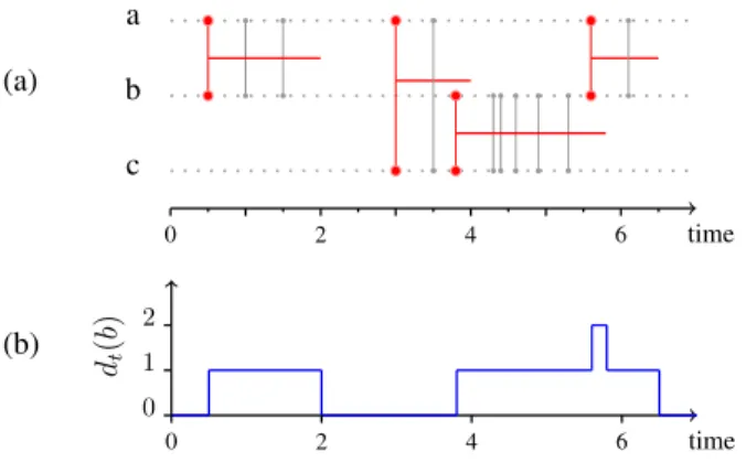
Fig. 1:Link stream for the modelling of IP traffic
-(a) Example of a link stream L = (T, V, E) formed from the
set of triplets D = {(1, a, b), (1.5, a, b), (3.5, a, c), (4.3, b, c),
(4.4, b, c), (4.6, b, c), (4.9, b, c), (5.3, b, c), (6.1, a, b)}:
T = [0, 7[, V = {a, b, c}, E = ( [0.5, 2[ ∪ [5.5, 6.5[ ) × {ab} ∪ [3, 4[ × {ac} ∪ [3.8, 5.8[ × {bc}. In the example, a interacts
with b from t1= 0.5 to t2 = 2. (b) Time evolution of the degree of
node b.
linked together from time t1 to time t2 if they exchanged
at least one packet every second within this time interval. Formally, L = (T, V, E) is defined by a time interval T ⊂ R, a set of nodes V and a set of links E ⊆ T × V ⊗ V where V ⊗ V denotes the set of unordered pairs of distinct elements of V , denoted by uv for any u and v in V (thus, uv ∈ V ⊗ V if and only if u, v ∈ V and u 6= v, and we make no distinction between uv and vu). If (t, uv) ∈ E then u and v are linked together at time t. In our case,
E = ∪(t,u,v)∈D[t − 12, t +
1
2[×{uv}. See Figure 1.a for an
illustration.
In L, the degree of (t, v) ∈ T × V , denoted by dt(v), is the
number of distinct nodes with which v interacts at time t:
dt(v) = |{u, (t, uv) ∈ E}|.
Figure 1.b shows the degree of node b over time.
IV. HETEROGENEITY OFDEGREES
In order to find events in a link stream using the degree, we first need to characterize the normal behaviour of couples (t, v) with respect to this feature. Then, a couple (t, v) ∈ T × V having a significantly different degree from the one of others would indicate an event: v interacts with an unusually high number of nodes at time t.
For this purpose, we call degree distribution of L the
fraction f (k) of couples (t, v) ∈ T × V for which dt(v) = k,
for all k:
f (k) =|{(t, v) ∈ T × V : dt(v) = k}|
|T × V | .
Figure 2 shows that the degree distribution is very
behaviour. In this situation, one may hardly identify values of degree that could be considered anomalous. Indeed, in such heterogeneous distributions, the mean and the standard deviation, which characterize the statistical normal behaviour, are not good estimators.
10−16 10−14 10−12 10−10 10−8 10−6 10−4 10−2 100 101 102 103 104 105 Fraction of (t, v ) s.t. dt (v ) = k Fraction of (t, v ) s.t. dt (v ) > k Degree k
Fig. 2: Degree distribution and complementary cumulative
de-gree distribution over L. For all (t, v) ∈ T × V , we compute the
degree dt(v) and plot the distribution of obtained values. The fraction
expresses the probability to draw a time instant t ∈ T and a node
v ∈ V such that dt(v) = k.
In order to circumvent this global heterogeneity, we observe degrees on sub-streams corresponding to IP traffic during time
slices of two seconds. Formally, we call Ti= [2i, 2i + 2[ the
ithtime slice, for all i ∈ {0, . . . , 1799} such that T0= [0, 2]
and T1799= [3598, 3600[, and we define
fi(k) =
|{(t, v) ∈ Ti× V : dt(v) = k}|
|Ti× V |
,
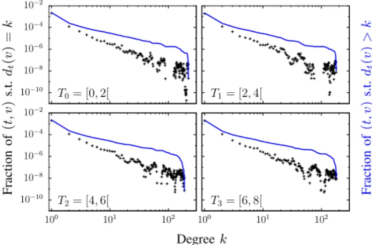
the degree distribution of the ith time slice. Figure 3 shows
that these distributions also are heterogeneous.
However, Figure 3 also shows that degree distributions fi
have similar shapes. To quantify this similarity, we fit them
with a power law model, y ∝ xa, where we estimate the
power law exponents by using linear fits of the distributions in which both coordinates are log-transformed. Other more complex and accurate techniques to fit power laws exist, see for instance [7]. Note that, in our context, the goodness of the fit is not the outcome of greatest interest. We are interested in knowing whether the parameters are similar on all time slices or not, not in values taken by parameters. We see on Figure 4 that linear model parameters are homogeneously distributed, suggesting that even if nodes have behaviours that are not comparable with each other, their overall behaviour is comparable from one time slice to another. We also see outlier values, distant from the mean, which in turn indicate changes in the overall behaviour on particular sub-streams. Using these observations, we design an outlier detection method based on temporal homogeneity of heterogeneous degree distributions. 10−10 10−8 10−6 10−4 10−2 T0= [0, 2[ T1= [2, 4[ 10−10 10−8 10−6 10−4 10−2 100 101 102 T2= [4, 6[ 100 101 102 T3= [6, 8[ Fraction of (t, v ) s.t. dt (v ) = k Fraction of (t, v ) s.t. dt (v ) > k Degree k
Fig. 3: Degree distribution and complementary cumulative
degree distribution over 2-seconds time slices. For T0= [0, 2[,
T1= [2, 4[, T2= [4, 6[ and T3= [6, 8[, we compute the degree dt(v)
for all (t, v) in the corresponding sub-stream and plot the distribution of obtained values. The fraction expresses the probability to draw a
time instant t ∈ Ti and a node v ∈ V such that dt(v) = k.
0 0.05 0.1 0.15 0.2 0.25 −3.75 −3 −2.25 −1.5 −0.75 0 Fraction of Ti s.t a = x
Linear model parametera,x
0 0.05 0.1 0.15 0.2 0.25 −10 −8 −6 −4 −2 Fraction of Ti s.t b = x
Linear model parameterb,x
Fig. 4:Similarity of degree distributions on different time slices.
For each Ti, we fit the degree distribution fiafter taking the log of
both coordinates using a linear model of the form y = ax + b. On the left is the distribution of parameter a on all time slices. On the right, the one of parameter b.
V. LEVERAGINGTEMPORALHOMOGENEITY TODETECT
EVENTS
The above observations lead to the following conclusion: degree distributions are heterogeneous in the same way on most, if not all, time slices. In other words, in each time slice, the fraction of couples (t, v) that have a given degree is similar to this fraction in other time slices. This is what we will consider as normal. Anomalies, instead, correspond to significant deviation from the usual fraction of nodes having a given degree. In this section we describe our method to compare degree distributions on all time slices and its use for outlier detection in our dataset.
First, notice that it makes little sense to consider the fraction of couples (t, v) having a degree exactly k when k is large: having degree k − 1 or k + 1 makes no significant difference.
Therefore, we define degree classes Cj and consider the
fraction of couples (t, v) having degrees in Cj, for all j:
fi(Cj) =
|{(t, v) ∈ Ti× V : dt(v) ∈ Cj}|
|Ti× V |
0 0.1 0.2 0.3 0.4 0.5 5.0 · 10−31.0 · 10−21.5 · 10−22.0 · 10−22.5 · 10−2 Fraction of Ti s.t fi (C 1 ) = x Fraction x of (t, v) ∈ C1 C1= {1} 0 0.02 0.04 0.06 0.08 0.1 0.12 0.14 8.0 · 10−5 1.2 · 10−4 1.6 · 10−4 Fraction of Ti s.t fi (C 2 ) = x Fraction x of (t, v) ∈ C2 C2= {2} 0 0.02 0.04 0.06 0.08 0.1 0.12 0 5.0 · 10−7 1.0 · 10−6 1.5 · 10−6 2.0 · 10−6 Fraction of Ti s.t fi (C 19 ) = x Fraction x of (t, v) ∈ C19 C19= {126, . . . , 158} 0 0.1 0.2 0.3 0.4 0.5 0.6 0.7 0.8 0.9 1 0 2.0 · 10−74.0 · 10−76.0 · 10−78.0 · 10−7 Fraction of Ti s.t fi (C 22 ) = x Fraction x of (t, v) ∈ C22 C22= {252, . . . , 315} 0 0.1 0.2 0.3 0.4 0.5 0.6 0.7 0.8 0.9 1 0 2.0 · 10−7 4.0 · 10−7 6.0 · 10−7 Fraction of Ti s.t fi (C 31 ) = x Fraction x of (t, v) ∈ C31 C31= {1996, . . . , 2510} 0 0.1 0.2 0.3 0.4 0.5 0.6 0.7 0.8 0.9 1 0 2.0 · 10−7 4.0 · 10−7 6.0 · 10−7 8.0 · 10−7 Fraction of Ti s.t fi (C 41 ) = x Fraction x of (t, v) ∈ C41 C41= {19953, . . . , 25118}
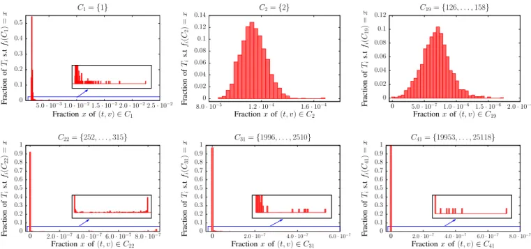
Fig. 5: Distributions of fractions fi(C) on all time slices Tifor degree class C in {C1, C2, C19, C22, C31, C41} - Distributions on C1,
C2 and C19are homogeneous with outliers. Distributions on C22, C31 and C41are peaked on zero since in most time slices there are no
couple (t, v) in the corresponding class.
Many options regarding the definition of Cj may make
sense. It seems crucial, however, to distinguish between degree 1 and degree 2, as well as to take into account the heterogeneity of degrees. Therefore, we choose to group them into classes of logarithmic scale. We define here the
jth degree class, C
j = {dkje, . . . , bkj+1c − 1} such that
k1 = 1 and log(kj+1) = log(kj) + 0.1, which leads to
C1 = {1}, C2 = {2}, C3 = {3}, C4 = {4, 5}, etc., until
C41= {19953, . . . , 25117}. We leave the exploration of other
class constructions for future works.
In order to compare degree distributions, we plot for a
given degree class C, the distribution on all time slices Ti
of the fraction fi(C). In other words, we study how the
fraction of couples (t, v) having degrees within C during
Ti is distributed among all time slices. Figure 5 shows the
distributions for classes C1, C2, C19, C22, C31 and C41.
In accordance with temporal homogeneity, we can see that most fractions are distributed around the mean and that a few only are distant from it. As expected according to the heterogeneity of degrees, the higher the degree class, the lower the fraction of couples (t, v) within the class. We see
on C1 that the average fraction over all time intervals is
2.1 · 10−3. When switching to C2, it drops to 1.15 · 10−4 and
gradually decreases to reach 0 in classes of degrees above 252. In these high degree classes, there is a peak on fraction 0, indicating that in most time slices the normality is that there is no couple (t, v) which have a degree reaching these classes.
In order to validate fractions fi homogeneity over time
0 0.02 0.04 0.06 0.08 0.1 0.12 0.14 8.0 · 10−5 1.2 · 10−4 1.6 · 10−4 Fraction of Ti s.t fi (C 2 ) = x Fraction x of (t, v) ∈ C2 After Grubbs’test Before Grubbs’test Fit KS 0.04566
Fig. 6: Fit of the fractions distribution on C2 after removing
outliers with Grubbs’ test - The KS distance between the fit and the empirical distribution is below the critical value. Hence, according to our method, this distribution is flagged as an homogeneous distribution with outliers.
slices within each degree class, we fit their distributions with
a normal distribution model P (x) = √1
2πσ2e −1 2( x−µ σ ) 2 where values are normally distributed around a mean µ with a standard deviation σ. Deciding whether a given distribution is homogeneous with outliers or not may then be done as follows [17]: (1) iteratively remove outliers from the distribution with Grubbs’ test [8]; (2) fitting the resulting distribution with the normal model; (3) evaluate the goodness of the fit. We use Maximum Likelihood Estimation (MLE) to determine which model parameters fit the best the empirical distribution [6] and evaluate the goodness of the fit with the Kolmogorov-Smirnov (KS) distance between the empirical
0 500 1000 1500 2000 2500 3000 3500 4000 4500 1313 1314 1315 1316 1317 dt (a ) t C31 0 50 100 150 200 250 300 350 841 842 843 844 845 dt (b ) t C22
Fig. 7: Different patterns in fractions distributions within high
degree classes - On the left, the degree profile of node a shows
the transition of this node through C31 from a lower to a higher
degree class. It stays in this class very little time. Hence, the number of couples (t, v) involved is low which makes its contribution to
the fraction f657(C31) very low. On the right, the degree of node
b fluctuates within class C22 making its contribution to the fraction
f421(C31) maximal.
and the reference distributions [21]. In this framework, we find 37 distributions homogeneous with outliers among the 41 corresponding to each degree class (see Fig. 6). The remaining 4 are discarded from the study. One may use more complex and accurate techniques to automatically perform this decision, see for instance the work performed by Motulsky et al. [20].
Unlike heterogeneous distributions, homogeneous
distributions with outliers clearly exhibit statistical anomalies: most values are similar to a mean value (normality) but some significantly deviate from it (abnormality). Given an homogeneous distribution with outliers, we use here the classical assumption that a value is anomalous if its distance to the mean exceeds three times the standard deviation [5], [9]. For the first class containing degree 1 only, we obtain 151 time slices flagged as anomalous. Outliers are also found
in the following degree classes: 5 anomalous slices in C2and
12 in C19. In higher degree classes, peaked on 0, anomalous
values correspond to all values greater than 0. Among these,
we can distinguish two groups of anomalous fractions fi(C):
the ones that are close to 0 and the others, as we can see on classes 22 and 31 in Figure 5. These two groups of fractions often reflect the behaviour of single nodes. Indeed, while the transition of a node u through a given class, from a lower to a higher degree class, implies a small number of couples (t, u) and thus is often responsible of a low fraction, the stabilization of a node u in a class implies a lot of couples (t, u) which in turn is often responsible of a high fraction (see Fig. 7).
Finally, our method for event detection from degrees distribution is the following: we group degree values into degree classes of logarithmic width. For a given degree class C, we look at the distribution on all time slices of the fraction
fi(C). This distribution indicates anomalous values which
mean that there are anomalous high numbers of couples (t, v) having degree within C during specific time slices. We then call an anomalous value of this kind a detected event.
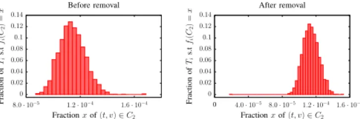
0 0.02 0.04 0.06 0.08 0.1 0.12 0.14 8.0 · 10−5 1.2 · 10−4 1.6 · 10−4 Fraction of Ti s.t fi (C 2 ) = x Fraction x of (t, v) ∈ C2 Before removal 0 0.02 0.04 0.06 0.08 0.1 0.12 0.14 0 4.0 · 10−5 8.0 · 10−5 1.2 · 10−4 1.6 · 10−4 Fraction of Ti s.t fi (C 2 ) = x Fraction x of (t, v) ∈ C2 After removal
Fig. 8: Distributions of the fractions on all time intervals over
C2 before and after the removal - The removal of all interactions
(t, uv) such that couples (t, v) have degree in C2during the detected
time slice T1080causes the appearance of a negative outlier.
A detected event gives two pieces of information: the time
slice Ti on which the anomalous value has been observed
and the degree class C in which the couple(s) responsible for the high fraction is or are located. At this stage, we detected 1,358 such events. We now address the goal of identifying the couples (t, v) in T × V responsible for these detected events.
VI. ITERATIVEREMOVAL TOIDENTIFYEVENTS
A detected event is a degree class C and a time slice Ti
such that the fraction fi(C) is unusually high compared to
the ones in other time slices. Identifying this event means recovering the set of couples (t, v) responsible for this anomaly. In this section, we introduce an iterative removal method and show that it leads to such identification.
Let’s take time slice T1080 detected in degree class C2
as an example. We have access to the set of couples (t, v)
which have a degree in C2 during T1080. However, we cannot
directly identify the event by this set. Indeed, let’s consider
the new link stream L0 such that L0 = (T, V, E0) with
E0 = E \ {(t, uv) : t ∈ T1080 and dt(v) ∈ C2}. We see on
Figure 8 that the removal of this set of interactions from the
link stream causes the appearance of a negative outlier2 in
the distribution of the fractions on C2. Thus, by removing all
interactions (t, uv) such that couples (t, v) have degree in C2
during T1080, we removed anomalous traffic but also normal
traffic. Therefore, identifying the detected event as the set
{(t, v) : t ∈ T1080 and dt(v) ∈ C2} is not accurate enough.
This suggest that one cannot directly identify couples acting abnormally in low degree classes. Indeed, in these classes, the normal fraction is greater than zero. Hence, an anomalous fraction consists in anomalous couples but also normal ones, which prevents us from identifying responsible couples only. On the contrary, in high degree classes the expected fraction is zero. Thus, couples (t, v) contributing to non-zero fractions are clearly anomalous. Events detected in such degree class C can therefore be correctly identified with
the set {(t, v) : t ∈ Ti and dt(v) ∈ C}.
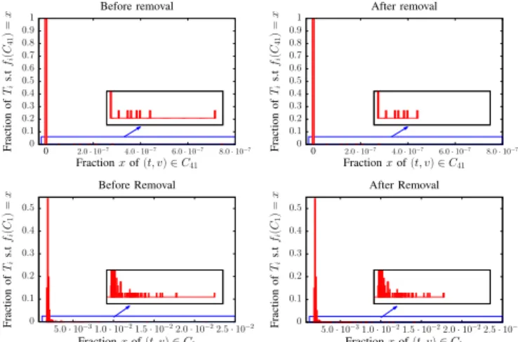
0 0.1 0.2 0.3 0.4 0.5 0.6 0.7 0.8 0.9 1 0 2.0 · 10−7 4.0 · 10−7 6.0 · 10−7 8.0 · 10−7 Fraction of Ti s.t fi (C 41 ) = x Fraction x of (t, v) ∈ C41 Before removal 0 0.1 0.2 0.3 0.4 0.5 0.6 0.7 0.8 0.9 1 0 2.0 · 10−7 4.0 · 10−7 6.0 · 10−7 8.0 · 10−7 Fraction of Ti s.t fi (C 41 ) = x Fraction x of (t, v) ∈ C41 After removal 0 0.1 0.2 0.3 0.4 0.5 5.0 · 10−31.0 · 10−21.5 · 10−22.0 · 10−22.5 · 10−2 Fraction of Ti s.t fi (C 1 ) = x Fraction x of (t, v) ∈ C1 Before Removal 0 0.1 0.2 0.3 0.4 0.5 5.0 · 10−31.0 · 10−21.5 · 10−22.0 · 10−22.5 · 10−2 Fraction of Ti s.t fi (C 1 ) = x Fraction x of (t, v) ∈ C1 After Removal
Fig. 9:Event identification in high degree classes - The removal
of an identified event in the high degree class C41 allows the
identification of an event detected in the lower degree class C1.
Consequently, we now consider degree class C41 on
which the normal fraction is 0. Its larger anomalous fraction
corresponds to time slice T315. Hence, this event can be
identified by the set {(t, v) : t ∈ T315 and dt(v) ∈ C41}.
Figure 9 shows the consequences of its removal. As
expected, the anomalous fraction in C41 vanishes without
creating a negative outlier. Additionally, one may notice the
disappearance of an outlier in C1. By looking into the data,
we can see that the removed set corresponds to a single node, u, whose neighbours all have degree 1. Thus, the outlier that
disappears in C1 was, in fact, caused by the high number
of neighbours of u. The removal of u and the one of its
interactions then lead to the identification of the event in C1
by the set {(t, v) : t ∈ T315and v ∈ Nt(u)}.
Finally, our approach for event identification consists in removing one by one correctly identified events in high degree classes. We repeat this operation until we reach classes of degree in which outliers contain anomalous traffic as well as normal traffic. This iterative process, in addition to removing anomalous traffic identified in high degree classes, allows to identify related events in lower classes as well. If a given removal creates a negative outlier in a degree class, this means that we removed too much. The removal that caused it is then cancelled and the corresponding event stays detected but unidentified.
In our dataset, none of the removals generated negative outliers. Altogether, we directly identified and removed 205 events in high degree classes. These removals allowed us to identify a total of 1, 163 outliers on the 1, 358 previously detected ones, hence more than 85% of detected outliers. We
can see in Figure 10 the final shape of classes C1 and C2
in which almost all outliers disappeared. Figure 11 shows the degree profiles of 4 nodes which have been removed for time periods during which they were acting abnormally. In
particular, node v1, for which the degree fluctuates within
0 0.02 0.04 0.06 0.08 0.1 0.12 1.8 · 10−3 1.9 · 10−3 2.1 · 10−3 Fraction of Ti s.t fi (C 1 ) = x Fraction x of (t, v) ∈ C1 C1= {1} 0 0.02 0.04 0.06 0.08 0.1 8.0 · 10−5 1.0 · 10−4 1.2 · 10−4 1.4 · 10−4 Fraction of Ti s.t fi (C 2 ) = x Fraction x of (t, v) ∈ C2 C2= {2}
Fig. 10:Distributions of the fractions on all time slices for degree
classes C1 and C2 after events removals - Before events removals
there were 151 anomalous values in C1 and 5 in C2. After the
removals, it only remains 10 unidentified anomalous values in C1
and 2 in C2. 0 75 150 225 300 v1 0 750 1500 2250 3000 v2 0 3.0 · 103 6.0 · 103 9.0 · 103 1.2 · 104 1.5 · 104 0 750 1500 2250 3000 v3 0 750 1500 2250 3000 0 150 300 450 600 v4 De gree Time t
Fig. 11: Degree profiles of 4 identified nodes - v1 is responsible
for the high probability on the largest fraction on C22. The set
{(t, v1) : t ∈ [712, 940[ and dt(v) ∈ C22} has been identified
and removed. v2 has a normal activity with a degree around 160
and a sharp variation on T223 = [446, 448[. The set {(t, v2) : t ∈
T223 and dt(v) ∈ C32} has been identified and removed. However,
normal interactions of v2during this time interval were also removed.
The degree of v3 reaches several powers of two which indicates that
this node is running network scans [11]. The sets {(t, v3)} where v3
is active have all been identified and removed. For the node v4, the
four peaks corresponding to degree values higher than 300 has been identified and removed.
C22, contributes identically and maximally to the fractions x
of couples (t, v) within this class during the corresponding interval. This makes it responsible for the peak on fraction
8.5 · 10−7 observed in C22 on Figure 5. As expected, we
notice the disappearance of this outlier after the removal of v1.
VII. DISCUSSION ANDCONCLUSION
In this paper, we introduced a method to detect outliers in IP traffic modelled as a link stream by studying the degree of each node over time. To deal with degrees heterogeneity we designed a method in two steps. First, we introduced a procedure to compare heterogeneous degree distributions over different time slices. From there we detected events during anomalous time slices and in specific degree classes. Thanks to these temporal and structural informations about the event,
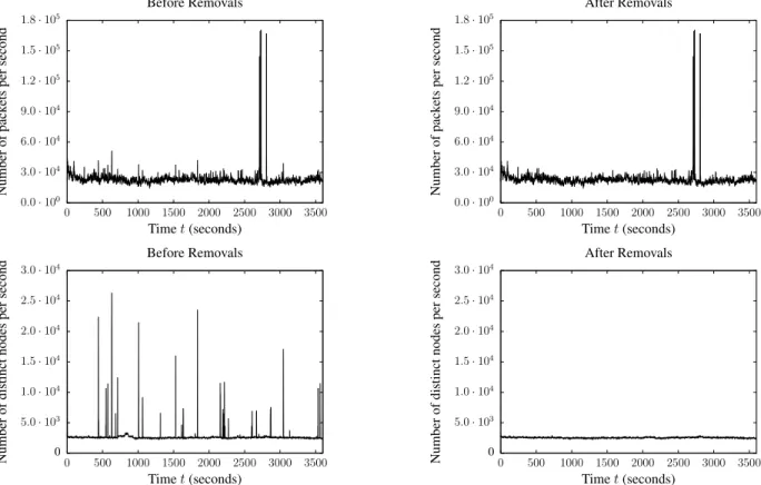
0.0 · 100 3.0 · 104 6.0 · 104 9.0 · 104 1.2 · 105 1.5 · 105 1.8 · 105 0 500 1000 1500 2000 2500 3000 3500 Number of pack ets per second Time t (seconds) Before Removals 0.0 · 100 3.0 · 104 6.0 · 104 9.0 · 104 1.2 · 105 1.5 · 105 1.8 · 105 0 500 1000 1500 2000 2500 3000 3500 Number of pack ets per second Time t (seconds) After Removals 0 5.0 · 103 1.0 · 104 1.5 · 104 2.0 · 104 2.5 · 104 3.0 · 104 0 500 1000 1500 2000 2500 3000 3500 Number of distinct nodes per second Time t (seconds) Before Removals 0 5.0 · 103 1.0 · 104 1.5 · 104 2.0 · 104 2.5 · 104 3.0 · 104 0 500 1000 1500 2000 2500 3000 3500 Number of distinct nodes per second Time t (seconds) After Removals
Fig. 12: Consequences of events removals on the number of packets per second and the number of distinct nodes per second - In
both cases, our method succeeds in removing identified anomalies with no significant impact on the underlying normal traffic. Peaks in the number of packets per second are less affected than those of the number of distinct IP per second since the first feature is less correlated with the degree.
we were then able to identify couples (t, v) responsible for this anomaly but only in high degree classes. Hence, we then introduced an event identification procedure relying on an iterative removal of events identified in these high degree classes. This last steps allowed us to trace back responsible IP addresses and instants in low degree classes as well.
The results we obtained show that our method allows to find interesting anomalous activities in IP traffic. In particular, we found point to multipoint anomalies and network scans as
for instance node v3in Figure 11. More generally, our method
succeeds in finding anomalous couples (t, v) independently of their degree’s order of magnitude. Hence, a node having a constant degree will not be identified as anomalous on any time slice even if its degree is much larger than other nodes. It will however detect couples (t, v) acting abnormally compared to what others do on other time slices. These results could not have been obtained by studying degree variations for all couples (t, v) ∈ T × V . Indeed, studying this feature leads to the same heterogeneity problem: there are nodes that suddenly interact with twice more neighbours, as well as 5 or 100, etc., times more. Hence, we are still confronted with different orders of magnitude and consequently to heterogeneous distributions.
Figure 12 shows the number of packets per second and the number of distinct nodes per second before and after applying our method. These two features are distributed homogeneously with outliers on all seconds within T . However an outlier only tells us that there are seconds during which the number of packets, or the number of distinct nodes, respectively, is larger than usual. Hence, the event is detected but not identified since we cannot trace back responsible nodes nor
instants with these distributions only.3 After removing the
events identified with our method, we see that peaks as well as sudden changes in the trends disappear without altering the underlying normal traffic. This means that our method enables us to identify events in other measurements where anomalies had been detected but not identified. In particular for the number of distinct nodes per second, for each outliers in the distribution we know which couples (t, v) caused it. This last result is particularly promising: it shows that by using more complex metrics, it is possible to identify events previously detected but unidentified with simpler metrics. The 195 events that we have not been able to identify with
3Nodes cannot be identified by newly appeared nodes of degree 1 after
the detection of an anomaly. Indeed, the number of new nodes of degree 1 appearing in each sub-stream is much larger than the number of nodes causing the anomaly.
the degree could therefore be identified in future works by using other features of the link streams.
This work however only is a first step towards anomaly detection in link streams and may be improved on several aspects. In particular, some removals delete anomalous traffic as well as normal traffic without creating a negative outlier. This is the case, for instance, when a node u has a normal activity with a non-zero degree and a sudden change on a
time slice as for node v2 in Figure 11. Degree allows to
detect couples (t, u) but not specific links (t, uv). Hence, by removing the set of identified couples (t, u) during the detected time slice, we remove u’s anomalous interactions as well as u’s normal interactions. This last point could be improved by considering more complex features than the degree, defined on the set of interactions E instead of the set of couples T × V . Many details may also be improved, especially the choice of parameters and modelling hypothesis, like for instance: the fact that we linked nodes together if they exchanged packets at least every second; the fact that we considered undirected links; or the effects of classes sizes on the results. One may also explore other choices for the duration of time intervals on which we compare degree distributions.
The next logical step of this work would be to extend our method with more complex features than the degree in order to find more complex anomalies as well and identify the remaining events unidentified with the degree. This task would be simplified by the fact that largest anomalies have already been removed from the remaining traffic, allowing a more detailed and finer analysis. At broader scale, our work could be useful in the field of IP traffic modelling as we would be able to generate normal traffic according to a specific feature. Likewise, thanks to their individual extraction, anomalies could also be studied separately.
ACKNOWLEDGEMENT
This work is funded in part by the European Commission H2020 FETPROACT 2016-2017 program under grant 732942 (ODYCCEUS), by the ANR (French National Agency of Research) under grants ANR-15- E38-0001 (AlgoDiv), by the Ile-de-France Region and its program FUI21 under grant 16010629 (iTRAC).
REFERENCES
[1] E. Anceaume and Y. Busnel. Sketch*-metric: Comparing data streams via sketching. In Network Computing and Applications (NCA), 2013 12th IEEE International Symposium on, pages 25–32. IEEE, 2013.
[2] H. Asai, K. Fukuda, P. Abry, P. Borgnat, and H. Esaki. Network
application profiling with traffic causality graphs. International Journal of Network Management, 24(4):289–303, 2014.
[3] P. Barford, J. Kline, D. Plonka, and A. Ron. A signal analysis of network traffic anomalies. In Proceedings of the 2nd ACM SIGCOMM Workshop on Internet measurment, pages 71–82. ACM, 2002.
[4] P. Borgnat, G. Dewaele, K. Fukuda, P. Abry, and K. Cho. Seven years and one day: Sketching the evolution of internet traffic. In INFOCOM 2009, IEEE, pages 711–719. IEEE, 2009.
[5] V. Chandola, A. Banerjee, and V. Kumar. Anomaly detection: A survey. ACM computing surveys (CSUR), 41(3):15, 2009.
[6] S. R. Eliason. Maximum likelihood estimation: Logic and practice,
volume 96. Sage Publications, 1993.
[7] M. L. Goldstein, S. A. Morris, and G. G. Yen. Problems with fitting
to the power-law distribution. The European Physical Journal
B-Condensed Matter and Complex Systems, 41(2):255–258, 2004. [8] F. E. Grubbs. Procedures for detecting outlying observations in samples.
Technometrics, 11(1):1–21, 1969.
[9] J. Han, J. Pei, and M. Kamber. Data mining: concepts and techniques. Elsevier, 2011.
[10] C. R. Harshaw, R. A. Bridges, M. D. Iannacone, J. W. Reed, and J. R. Goodall. Graphprints: Towards a graph analytic method for network
anomaly detection. In Proceedings of the 11th Annual Cyber and
Information Security Research Conference, page 15. ACM, 2016.
[11] H. Huang, H. Al-Azzawi, and H. Brani. Network traffic anomaly
detection. arXiv preprint arXiv:1402.0856, 2014.
[12] M. Iliofotou, M. Faloutsos, and M. Mitzenmacher. Exploiting dynam-icity in graph-based traffic analysis: techniques and applications. In Proceedings of the 5th international conference on Emerging networking experiments and technologies, pages 241–252. ACM, 2009.
[13] A. Kato, J. Murai, S. Katsuno, and T. Asami. An internet traffic
data repository: The architecture and the design policy. In INET’99 Proceedings, 1999.
[14] T. La Fond, J. Neville, and B. Gallagher. Anomaly detection in dynamic networks of varying size. arXiv preprint arXiv:1411.3749, 2014. [15] A. Lakhina, M. Crovella, and C. Diot. Characterization of network-wide
anomalies in traffic flows. In Proceedings of the 4th ACM SIGCOMM conference on Internet measurement, pages 201–206. ACM, 2004. [16] A. Lakhina, M. Crovella, and C. Diot. Diagnosing network-wide traffic
anomalies. In ACM SIGCOMM Computer Communication Review,
volume 34, pages 219–230. ACM, 2004.
[17] M. Latapy, A. Hamzaoui, and C. Magnien. Detecting events in the dynamics of ego-centred measurements of the internet topology. Journal of Complex Networks, 2(1):38–59, 2013.
[18] M. Latapy, T. Viard, and C. Magnien. Stream graphs and link streams for the modeling of interactions over time. arXiv preprint arXiv:1710.04073, 2017.
[19] W. Lee, S. J. Stolfo, et al. Data mining approaches for intrusion
detection. In USENIX Security Symposium, pages 79–93. San Antonio, TX, 1998.
[20] H. J. Motulsky and R. E. Brown. Detecting outliers when fitting data with nonlinear regression–a new method based on robust nonlinear regression and the false discovery rate. BMC bioinformatics, 7(1):123, 2006.
[21] W. H. Press, S. A. Teukolsky, W. T. Vetterling, and B. P. Flannery. Numerical recipes in c: The art of scientific computing. second edition, 1992.
[22] H. Ringberg, A. Soule, J. Rexford, and C. Diot. Sensitivity of pca for traffic anomaly detection. ACM SIGMETRICS Performance Evaluation Review, 35(1):109–120, 2007.
[23] T. A. Schieber, L. Carpi, A. D´ıaz-Guilera, P. M. Pardalos, C. Masoller, and M. G. Ravetti. Quantification of network structural dissimilarities. Nature communications, 8:13928, 2017.
[24] J. Tajer, M. Adda, and B. Aziz. Comparison between divergence
measures for anomaly detection of mobile agents in ip networks. International Journal of Wireless & Mobile Networks (IJWMN), 9(3), 2017.
[25] T. Viard, R. Fournier-S’niehotta, C. Magnien, and M. Latapy. Discover-ing patterns of interest in ip traffic usDiscover-ing cliques in bipartite link streams. In Proceedings of the International Conference on Complex Networks (CompleNet), 2018.
[26] N. Williams, S. Zander, and G. Armitage. A preliminary performance comparison of five machine learning algorithms for practical ip traffic flow classification. ACM SIGCOMM Computer Communication Review, 36(5):5–16, 2006.
[27] K. Xu, F. Wang, and L. Gu. Behavior analysis of internet traffic via bipartite graphs and one-mode projections. IEEE/ACM Transactions on Networking, 22:931–942, 2014.