HAL Id: hal-01320498
https://hal.archives-ouvertes.fr/hal-01320498
Submitted on 23 May 2016
HAL is a multi-disciplinary open access
archive for the deposit and dissemination of
sci-entific research documents, whether they are
pub-lished or not. The documents may come from
teaching and research institutions in France or
abroad, or from public or private research centers.
L’archive ouverte pluridisciplinaire HAL, est
destinée au dépôt et à la diffusion de documents
scientifiques de niveau recherche, publiés ou non,
émanant des établissements d’enseignement et de
recherche français ou étrangers, des laboratoires
publics ou privés.
Optimal control of infinite-dimensional piecewise
deterministic Markov processes and application to the
control of neuronal dynamics via Optogenetics
Vincent Renault, Michèle Thieullen, Emmanuel Trélat
To cite this version:
Vincent Renault, Michèle Thieullen, Emmanuel Trélat. Optimal control of infinite-dimensional
piece-wise deterministic Markov processes and application to the control of neuronal dynamics via
Opto-genetics. Networks and Heterogeneous Media, AIMS-American Institute of Mathematical Sciences,
2017, 12 (3), pp.417–459. �hal-01320498�
Optimal control of infinite-dimensional piecewise
deterministic Markov processes and application to the
control of neuronal dynamics via Optogenetics
Vincent Renault, Michèle Thieullen
⇤, Emmanuel Trélat
†Abstract
In this paper we define an infinite-dimensional controlled piecewise deterministic Markov process (PDMP) and we study an optimal control problem with finite time horizon and unbounded cost. This process is a coupling between a continuous time Markov Chain and a set of semilinear parabolic partial differential equations, both processes depending on the control. We apply dynamic programming to the embedded Markov decision process to obtain existence of optimal relaxed controls and we give some sufficient conditions ensuring the existence of an optimal ordinary control. This study, which constitutes an extension of controlled PDMPs to infinite dimension, is motivated by the control that provides Optogenetics on neuron models such as the Huxley model. We define an infinite-dimensional controlled Hodgkin-Huxley model as an infinite-dimensional controlled piecewise deterministic Markov process and apply the previous results to prove the existence of optimal ordinary controls for a tracking problem.
Keywords. Piecewise Deterministic Markov Processes, optimal control, semilinear parabolic equations, dynamic programming, Markov Decision Processes, Optogenetics.
AMS Classification. 93E20. 60J25. 35K58. 49L20. 92C20. 92C45.
Introduction
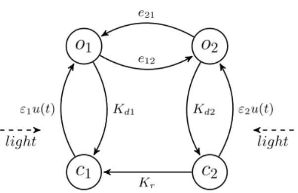
Optogenetics is a recent and innovative technique which allows to induce or prevent electric shocks in living tissues, by means of light stimulation. Successfully demonstrated in mammalian neurons in 2005 ([8]), the technique relies on the genetic modification of cells to make them express par-ticular ionic channels, called rhodopsins, whose opening and closing are directly triggered by light stimulation. One of these rhodopsins comes from an unicellular flagellate algae, Chlamydomonas reinhardtii, and has been baptized Channelrodhopsins-2 (ChR2). It is a cation channel that opens when illuminated with blue light.
Since the field of Optogenetics is young, the mathematical modeling of the phenomenon is quite scarce. Some models have been proposed, based on the study of the photocycles initiated by the absorption of a photon. In 2009, Nikolic and al. [37] proposed two models for the ChR2 that are able to reproduce the photocurrents generated by the light stimulation of the channel. Those models are constituted of several states that can be either conductive (the channel is open) or non-conductive (the channel is closed). Transitions between those states are spontaneous, depend on the membrane potential or are triggered by the absorption of a photon. For example, the four-states model of Nikolic and al. [37] has two open states (o1 and o2) and two closed states (c1
and c2). Its transitions are represented on Figure 1
⇤Sorbonne Universités, UPMC Univ Paris 06, CNRS UMR 7599, Laboratoire de Probabilités et Modèles
Aléa-toires, F-75005, Paris, France. email: vincent.renault@upmc.fr, michele.thieullen@upmc.fr
†Sorbonne Universités, UPMC Univ Paris 06, CNRS UMR 7598, Laboratoire Jacques-Louis Lions, Institut
o
1o
2c
2c
1 Kd1 e12 e21 Kd2 "2u(t) Kr "1u(t) light lightFigure 1: Simplified four states ChR2 channel : "1, "2, e12, e21, Kd1, Kd2 and Kr are positive
constants.
The purpose of this paper is to extend to infinite dimension the optimal control of Piecewise De-terministic Markov Processes (PDMPs) and to define an infinite-dimensional controlled Hodgkin-Huxley model, containing ChR2 channels, as an infinite-dimensional controlled PDMP and prove existence of optimal ordinary controls. We now give the definition of the model.
We consider an axon, described as a 1-dimensional cable and we set I = [0, 1] (the more physical case I = [ l, l] with 2l > 0 the length of the axon is included here by a scaling argument). Let DChR2 :={o1, o2, c1, c2}. Individually, a ChR2 features a stochastic evolution which can be
properly described by a Markov Chain on the finite space constituted of the different states that the ChR2 can occupy. In the four-states model above, two of the transitions are triggered by light stimulation, in the form of a parameter u that can evolve in time. Here u(t) is physically proportional to the intensity of the light with which the protein is illuminated. For now, we will consider that when the control is on (i.e., when the light is on), the entire axon is uniformly illuminated. Hence for all t 0, u(t) features no spatial dependency.
The deterministic Hodgkin-Huxley model was introduced in [33]. A stochastic infinite-dimensional model was studied in [4], [10], [31] and [43]. The Sodium (Na+) channels and Potassium (K+)
channels are described by two pure jump processes with state spaces D1 := {n0, n1, n2, n3, n4}
and
D2:={m0h1, m1h1, m2h1, m3h1, m0h0, m1h0, m2h0, m3h0}.
For a given scale N 2 N⇤, we consider that the axon is populated by N
hh= N 1channels of type
N a+, K+or ChR2, at positions 1
N(Z \ N˚I). In the sequel we will use the notation IN :=Z \ N˚I. We consider the Gelfand triple (V, H, V⇤) with V := H1
0(I)and H := L2(I). The process we study
is defined as a controlled infinite-dimensional Piecewise Deterministic Markov Process (PDMP). All constants and auxiliary functions in the next definition will be defined further in the paper. Definition 0.1. Stochastic controlled infinite-dimensional Hodgkin-Huxley-ChR2 model. Let N 2 N⇤. We call Nth stochastic controlled infinite-dimensional Hodgkin-Huxley-ChR2 model
the controlled PDMP (v(t), d(t)) 2 V ⇥ DN defined by the following characteristics:
• A state space V ⇥ DN with DN = DIN and D = D1[ D2[ DChR2.
• A control space U = [0, umax], umax> 0.
• A set of uncontrolled PDEs: For every d 2 DN,
(0.1) 8 > > < > > : v0(t) = 1 Cm v(t) + fd(v(t)), v(0) = v02 V, v0(x)2 [V , V+] 8x 2 I, v(t, 0) = v(t, 1) = 0, 8t > 0,
with D( ) = V, fd(v) := 1 N X i2IN ⇣ gK1{di=n4}(VK v( i N)) + gN a1{di=m3h1}(VN a v( i N)) (0.2) + gChR2(1{di=O1}+ ⇢1{di=O2})(VChR2 v( i N)) + gL(VL v( i N)) ⌘ i N,
with z2 V⇤ the Dirac mass at z 2 I.
• A jump rate function : V ⇥ DN⇥ U ! R+ defined for all (v, d, u) 2 H ⇥ DN⇥ U by
(0.3) d(v, u) = X i2IN X x2D X y2D, y6=x x,y(v( i N), u)1{di=x},
with x,y :R ⇥ U ! R⇤+ smooth functions for all (x, y) 2 D2. See Table 1 in Section 4.1 for
the expression of those functions.
• A discrete transition measure Q : V ⇥DN⇥U ! P(DN)defined for all (v, d, u) 2 E⇥DN⇥U
and y 2 D by (0.4) Q({di:y }|v, d) = di,y(v( i N), u)1{di6=y} d(v, u) ,
where di:y is obtained from d by putting its ith component equal to y.
From a biological point of view, the optimal control problem consists in mimicking an output signal that encodes a given biological behavior, while minimizing the intensity of the light applied to the neuron. For example, it can be a time-constant signal and in this case, we want to change the resting potential of the neuron to study its role on its general behavior. We can also think of pathological behaviors that would be fixed in this way. The minimization of light intensity is crucial because the range of intensity experimentally reachable is quite small and is always a matter of preoccupation for experimenters. These considerations lead us to formulate the following mathematical optimal control problem.
Suppose we are given a reference signal Vref 2 V . The control problem is then to find ↵ 2 A that
minimizes the following expected cost
(0.5) Jz(↵) =E↵z "Z T 0 ||X↵ t( ) Vref||2V + ↵(Xt↵) dt # , z2 ⌥,
where A is the space of control strategies, ⌥ an auxiliary state space that comprises V ⇥ DN, X·↵
is the controlled PDMP and X↵
· ( )its continuous component.
We will prove the following result.
Theorem 0.1. Under the assumptions of Section 1.1, there exists an optimal control strategy ↵⇤2 A such that for all z 2 ⌥,
Jz(↵⇤) = inf ↵2AE ↵ z "Z T 0 ||X↵ t( ) Vref||2V + ↵(Xt↵) dt # ,
and the value function z ! inf
Piecewise Deterministic Markov Processes constitute a large class of Markov processes suited to describe a tremendous variety of phenomena such as the behavior of excitable cells ([4],[10],[40]), the evolution of stocks in financial markets ([11]) or the congestion of communication networks ([23]), among many others. PDMPs can basically describe any non diffusive Markovian system. The general theory of PDMPs, and the tools to study them, were introduced by Davis ([18]) in 1984, at a time when the theory of diffusion was already amply developed. Since then, they have been widely investigated in terms of asymptotic behavior, control, limit theorems and CLT, numerical methods, among others (see for instance [9], [14], [15], [17] and references therein). PDMPs are jump processes coupled with a deterministic evolution between the jumps. They are fully described by three local characteristics: the deterministic flow , the jump rate , and the transition measure Q. In [18], the temporal evolution of a PDMP between jumps (i.e. the flow ) is governed by an Ordinary Differential Equation (ODE). For that matter, this kind of PDMPs will be referred to as finite-dimensional in the sequel.
Optimal control of such processes have been introduced by Vermes ([44]) in finite dimension. In [44], the class of piecewise open-loop controls is introduced as the proper class to consider to obtain strongly Markovian processes. A Hamilton-Jabobi-Bellman equation is formulated and necessary and sufficient conditions are given for the existence of optimal controls. The standard broader class of so-called relaxed controls is considered and it plays a crucial role in getting the existence of optimal controls when no convexity assumption is imposed. This class of controls has been studied, in the finite-dimensional case, by Gamkrelidze ([29]), Warga ([47] and [46]) and Young ([50]). Relaxed controls provide a compact class that is adequate for studying optimization problems. Still in finite dimension, many control problems have been formulated and studied such as optimal control ([28]), optimal stopping ([16]) or controllability ([32]). In infinite dimension, relaxed controls were introduced by Ahmed ([1], [2], [3]). They were also studied by Papageorgiou in [41] where the author shows the strong continuity of relaxed trajectories with respect to the relaxed control. This continuity result will be of great interest in this paper.
A formal infinite-dimensional PDMP was defined in [10] for the first time, the set of ODEs being replaced by a special set of Partial Differential Equations (PDE). The extended generator and its domain are provided and the model is used to define a stochastic spatial Hodgkin-Huxley model of neuron dynamics. The optimal control problem we have in mind here regards those Hodgkin-Huxley type models. Seminal work on an uncontrolled infinite-dimensional Hodgkin-Hodgkin-Huxley model was conducted in [4] where the trajectory of the infinite-dimensional stochastic system is shown to converge to the deterministic one, in probability. This type of model has then been studied in [43] in terms of limit theorems and in [31] in terms of averaging. The extension to infinite dimension heavily relies on the fact that semilinear parabolic equations can be interpreted as ODEs in Hilbert spaces.
To give a sense to Definition 0.1 and to Theorem 0.1, we will define a controlled infinite-dimensional PDMP for which the control acts on the three local characteristics. We consider controlled semi-linear parabolic PDEs, jump rates and transition measures Q depending on the control. This kind of PDE takes the form
˙x(t) = Lx(t) + f (x(t), u(t)),
where L is the infinitesimal generator of a strongly continuous semigroup and f is some function (possibly nonlinear). The optimal control problem we address is the finite-time minimization of an unbounded expected cost functional along the trajectory of the form
min
u E
Z T 0
c(x(t), u(t))dt,
where x(·) is the continuous component of the PDMP, u(·) the control and T > 0 the finite time horizon, the cost function c(·, ·) being potentially unbounded.
To address this optimal control problem, we use the fairly widespread approach that consists in studying the imbedded discrete-time Markov chain composed of the times and the locations of
the jumps. Since the evolution between jumps is deterministic, there exists a one-to-one cor-respondence between the PDMP and a pure jump process that enable to define the imbedded Markov chain. The discrete-time Markov chain belongs to the class of Markov Decision Processes (MDPs). This kind of approach has been used in [28] and [12] (see also the book [34] for a self-contained presentation of MDPs). In these articles, the authors apply dynamic programming to the MDP derived from a PDMP, to prove the existence of optimal relaxed strategies. Some sufficient conditions are also given to get non-relaxed, also called ordinary, optimal strategies. However, in both articles, the PDMP is finite dimensional. To the best of our knowledge, the optimal control of infinite-dimensional PDMPs has not yet been treated and this is one of our main objectives here, along with its motivation, derived from the Optogenetics, to formulate and study infinite-dimensional controlled neuron models.
The paper is structured as follows. In Section 1 we adapt the definition of a standard infinite-dimensional PDMP given in [10] in order to address control problems of such processes. To obtain a strongly Markovian process, we enlarge the state space and we prove an extension to controlled PDMPs of [10, Theorem 4]. We also define in this section the MDP associated to our controlled PDMP and that we study later on. In Section 2 we use the results of [41] to define relaxed controlled PDMPs and relaxed MDPs in infinite dimension. Section 3 gathers the main results of the paper. We show that the optimal control problems of PDMPs and of MDPs are equivalent. We build up a general framework in which the MDP is contracting. The value function is then shown to be continuous and existence of optimal relaxed control strategies is proved. We finally give in this section, some convexity assumptions under which an ordinary optimal control strategy can be retrieved.
The final Section 4 is devoted to showing that the previous theoretical results apply to the model of Optogenetics previously introduced. Several variants of the model are discussed, the scope of the theoretical results being much larger than the model of Definition 0.1.
1 Theoretical framework for the control of infinite-dimensional
PDMPs
1.1 The enlarged process and assumptions
In the present section we define the infinite-dimensional controlled PDMPs that we consider in this paper in a way that enables us to formulate control problems in which the three characteristics of the PDMP depend on an additional variable that we call the control parameter. In particular we introduce the enlarged process which enable us to address optimization problems in the subsequent sections.
Let (⌦, F, (Ft)t 0,P) be a filtered probability space satisfying the usual conditions. We consider a
Gelfand triple (V ⇢ H ⇢ V⇤) such that H is a separable Hilbert space and V a separable, reflexive
Banach space continuously and densely embedded in H. The pivot space H is identified with its dual H⇤, V⇤ is the topological dual of V . H is then continuously and densely embedded in V⇤.
We will denote by ||·||V, ||·||H, and ||·||V⇤ the norms on V , H, and V⇤, by (·, ·) the inner product
in H and by h·, ·i the duality pairing of (V, V⇤). Note that for v 2 V and h 2 H, hh, vi = (h, v).
Let D be a finite set, the state space of the discrete variable and Z a compact Polish space, the control space. Let T > 0 be the finite time horizon. Intuitively a controlled PDMP (vt, dt)t2[0,T ]
should be constructed on H ⇥ D from the space of ordinary control rules defined as A :={a : (0, T ) ! U measurable},
where U, the action space, is a closed subset of Z. Elements of A are defined up to a set in [0, T ] of Lebesgue measure 0. The control rules introduced above are called ordinary in contrast with the relaxed ones that we will introduce and use in order to prove existence of optimal strategies.
When endowed with the coarsest -algebra such that
a! Z T
0
e tw(t, a(t))dt
is measurable for all bounded and measurable functions w : R+⇥ U ! R, the set of control rules
A becomes a Borel space (see [51, Lemma 1]). This will be crucial for the discrete-time control problem that we consider later. Conditionally to the continuous component vt and the control
a(t), the discrete component dtis a continuous-time Markov chain given by a jump rate function
: H⇥ D ⇥ U ! R+ and a transition measure Q : H ⇥ D ⇥ U ! P(D).
Between two consecutive jumps of the discrete component, the continuous component vtsolves a
controlled semilinear parabolic PDE
(1.1)
(
˙vt= Lvt+ fd(vt, a(t)),
v0= v, v2 V.
For (v, d, a) 2 H ⇥ D ⇥ A we will denote by a(v, d)the flow of (1.1). Let T
n, n2 N be the jump
times of the PDMP. Their distribution is then given by
(1.2) P[dt+s= dt, 0 s t|dt] = exp Z t 0 ⇣ a t+s Tn(vTn, dTn), dt, a(t + s Tn) ⌘ ds ! ,
for t 2 [Tn; Tn+1). When a jump occurs, the distribution of the post jump state is given by
(1.3) P[dt= d|dt 6= dt] =Q({d}|dt, vt, a(t)).
The triple ( , Q, ) fully describes the process and is referred to as the local characteristics of the PDMP.
We will make the following assumptions on the local characteristics of the PDMP. (H( ))
For every d 2 D, d: H⇥ Z ! R+ is a function such that:
1. There exists M , > 0 such that:
d(x, z) M , 8(x, z) 2 H ⇥ Z.
2. z ! d(x, z) is continuous on Z, for all x 2 H.
3. x ! d(x, z)is locally Lipschitz continuous, uniformly in Z, that is, for every compact
set K ⇢ H, there exists l (K) > 0 such that
| d(x, z) d(y, z)| l (K)||x y||H 8(x, y, z) 2 K2⇥ Z.
(H(Q))
The function Q : H ⇥ D ⇥ Z ⇥ B(D) ! [0, 1] is a transition probability such that: (x, z) ! Q({p}|x, d, z) is continuous for all (d, p) 2 D2 (weak continuity) and Q({d}|x, d, z) = 0 for all (x, z) 2 H ⇥ Z.
(H(L))
L : V ! V⇤ is such that:
1. L is linear, monotone;
3. hLx, xi c2||x||2V, c2> 0;
4. Lgenerates a strongly continuous semigroup (S(t))t 0on H such that S(t) : H ! H
is compact for every t > 0. We will denote by MS a bound, for the operator norm, of
the semigroup on [0, T ]. (H(f))
For every d 2 D, fd : H⇥ Z ! H is a function such that:
1. x ! fd(x, z)is Lipschitz continuous, uniformly in Z, that is,
||fd(x, z) fd(y, z)||H lf||x y||H 8(x, z) 2 H ⇥ Z, lf > 0.
2. (x, z) ! fd(x, z) is continuous from H ⇥ Z to Hw, where Hw denotes the space H
endowed with the topology of weak convergence.
Let us make some comments on the assumptions above. Assumption (H( ))1. will ensure that the process is regular, i.e. the number of jumps of dtis almost surely finite in every finite time interval.
Assumption (H( ))2. will enable us to construct relaxed trajectories. Assumptions (H( ))3. and (H(Q)) will be necessary to obtain the existence of optimal relaxed controls for the associated MDP. Assumptions (H(L))1.2.3. (H(f)) will ensure the existence and uniqueness of the solution of (1.1). Note that all the results of this paper are unchanged if assumption (H(f))1 is replaced by
(H(f))’
For every d 2 D, fd : H⇥ Z ! H is a function such that:
1. x ! fd(x, z) is continuous monotone, for all z 2 Z.
2. ||fd(x, z)||H b1+ b2||x||H, b1 0, b2> 0, for all z 2 Z.
In particular, assumption (H(f)) implies (H(f))’2. and we will use the constants b1and b2further
in this paper. Note that they can be chosen uniformly in D since it is a finite set. To see this, note that z ! fd(0, z)is a weakly continuous on the compact space Z and thus weakly bounded.
It is then strongly bounded by the Uniform Boundedness Principle.
Finally, assumptions (H(f))3. and (H(L))4. will respectively ensure the existence of relaxed solutions of (1.1) and the strong continuity of theses solutions with regards to the relaxed control. For that last matter, the compactness of Z is also required. The following theorem is a reminder that the assumption on the semigroup does not make the problem trivial since it implies that L is unbounded when H is infinite-dimensional.
Theorem 1.1. (see [25, Theorem 4.29])
1. For a strongly continuous semigroup (T (t))t 0 the following properties are equivalent
(a) (T (t))t 0 is immediately compact.
(b) (T (t))t 0 is immediately norm continuous, and its generator has compact resolvent.
2. Let X be a Banach space. A bounded operator A 2 L(X) has compact resolvent if and only if X is finite-dimensional.
We define Uad((0, T ), U ) := {a 2 L1((0, T ), Z)|a(t) 2 U a.e.} ⇢ A the space of admissible rules.
Because of (H(L)) and (H(f)), for all a 2 Uad((0, T ), U ), (1.1) has a unique solution belonging to
L2((0, T ), V )\ H1((0, T ), V⇤)and moreover, the solution belongs to C([0, T ], H) (see [41] for the
construction of such a solution). We will make an extensive use of the mild formulation of the solution of (1.1), given by (1.4) a t(v, d) = S(t)v + Z t 0 S(t s)fd( as(v, d), a(s))ds,
with a
0(v, d) = v. One of the keys in the construction of a controlled PDMP in finite or infinite
dimension is to ensure that aenjoys the flow property a
t+s(v, d) = as( at(v, d), d)for all (v, d, a) 2
H⇥D⇥Uad((0, T ), U )and (t, s) 2 R+. It is the flow property that guarantees the Markov property
for the process. Under the formulation (1.4), it is easy to see that the solution a cannot feature
the flow property for any reasonable set of admissible rules. In particular, the jump process (dt, t 0)given by (1.2) and (1.3) is not Markovian. Moreover in control problems, and especially
in Markovian control problems, we are generally looking for feedback controls which depend only on the current state variable so that at any time, the controller needs only to observe the current state to be able to take an action. Feedback controls would ensure the flow property. However they impose a huge restriction on the class of admissible controls. Indeed, feedback controls would be functions u : H ⇥ D ! U and for the solution of (1.1) to be uniquely determined, the function x! fd(x, u(x, d))needs to be Lipschitz continuous. It would automatically exclude discontinuous
controls and therefore would not be adapted to control problems. To avoid this issue, Vermes introduced piecewise open-loop controls (see [44]): after a jump of the discrete component, the controller observes the location of the jump, say (v, d) 2 H ⇥ D and chooses a control rule a2 Uad((0, T ), U )to be applied until the next jump. The time elapsed since the last jump must
then be added to the state variable in order to see a control rule as a feedback control. While Vermes [44] and Davis [19] only add the last post jump location we also want to keep track of the time of the last jump in order to define proper controls for the Markov Decision Processes that we introduce in the next section, and to eventually obtain optimal feedback policies. According to these remarks, we now enlarge the state space and define control strategies for the enlarged process. We introduce first several sets that will be useful later on.
Definition 1.1. Let us define the following sets D(T, 2) := {(t, s) 2 [0, T ]2
| t + s T }, ⌅ := H⇥ D ⇥ D(T, 2) ⇥ H and ⌥ := H ⇥ D ⇥ [0, T ].
Definition 1.2. Control strategies. Enlarged controlled PDMP. Survival function. a) The set A of admissible control strategies is defined by
A := {↵ : ⌥ ! Uad([0, T ]; U ) measurable}.
b) On ⌅ we define the enlarged controlled PDMP (X↵
t)t 0 = (vt, dt, ⌧t, ht, ⌫t)t 0 with strategy
↵2 A as follows:
• (vt, dt)t 0 is the original PDMP,
• ⌧tis the time elapsed since the last jump at time t,
• ht is the time of the last jump before time t,
• ⌫tis the post jump location right after the jump at time ht.
c) Let z := (v, d, h) 2 ⌥. For a 2 Uad([0, T ]; U ) we will denote by a.(z)the solution of
d dt
a
t(z) = at(z) d( at(z), a(t)), a0(z) = 1,
and its immediate extension ↵
.(z)to A such that the process (Xt↵)t 0starting at (v, d, 0, h, v) 2 ⌅,
admits ↵ . as survival function: P[T1> t] = ↵t(z). The notation a t(z) means here a t(z) := S(t)v + Z t 0 S(t s)fd( as(z), a(s))ds. and ↵ t(z) means ↵ t(z) := S(t)v + Z t 0 S(t s)fd( as(z), ↵(z)(s))ds.
Remark 1.1. i)Thanks to [51, Lemma 3], the set of admissible control strategies can be seen as a set of measurable feedback controls acting on ⌅ and with values in U. The formulation of Definition 1.2 is adequate to address the associated discrete-time control problem in Section 1.3. ii) In view of Definition 1.2, given ↵ 2 A, the deterministic dynamics of the process (X↵
t)t 0 =
(vt, dt, ⌧t, , ht, ⌫t)t 0 between two consecutive jumps obeys the initial value problem
(1.5) 8 > > > > > > < > > > > > > : ˙vt= Lvt+ fd(vt, ↵(v, d, s)(⌧t)), vs= v2 E, ˙ dt= 0, ds= d2 D, ˙⌧t= 1, ⌧s= 0, ˙ht= 0, hs= s2 [0, T ], ˙⌫t= 0, ⌫s= vs= v,
with s the last time of jump. The jump rate function and transition measure of the enlarged PDMP are straightforwardly given by the ones of the original process and will be denoted the same (see Appendix A for their expression).
iii) If the relation t = ht+ ⌧tindicates that the variable htmight be redundant, recall that we keep
track of it on purpose. Indeed, the optimal control will appear as a function of the jump times so that keeping them as a variable will make the control feedback.
iv) Because of the special definition of the enlarged process, for every control strategy in A, the initial point of the process (X↵
t)t 0 cannot be any point of the enlarged state space ⌅. More
precisely we introduce in Definition 1.3 below the space of coherent initial points. Definition 1.3. Space of coherent initial points.
Take ↵ 2 A and x := (v0, d0, 0, h0, v0)2 ⌅ and extend the notation ↵t(x) of Definition 1.2 to ⌅
by ↵ t(x) := S(t)v0+ Z t 0 S(t s)fd0( ↵ s(x), ↵(v0, d0, h0)(⌧s))ds The set ⌅↵
⇢ ⌅ of coherent initial points is defined as follows
(1.6) ⌅↵:={(v, d, ⌧, h, ⌫) 2 ⌅ | v = ↵⌧(⌫, d, 0, h, ⌫)}.
Then we have for all x := (v0, d0, ⌧0, h0, ⌫0)2 ⌅↵,
↵ t(x) := S(t)v0+ Z t 0 S(t s)fd0( ↵ s(x), ↵(⌫0, d0, h0)(⌧s))ds Note that (X↵
t) can be constructed like any PDMP by a classical iteration that we recall in
Appendix A for the sake of completeness. Proposition 1.1. The flow property.
Take ↵ 2 A and x := (v0, d0, ⌧0, h0, ⌫0) 2 ⌅↵. Then ↵t+s(x) = ↵t( ↵s(x), ds, ⌧s, hs, ⌫s) for all
(t, s)2 R2 +.
Notation. Let ↵ 2 A. For z 2 ⌥, we will use the notation ↵s(z) := ↵(z)(s). Furthermore, we
will sometimes denote by Q↵(·|v, d) instead of Q(·|v, d, ↵⌧(⌫, d, h))for all (v, d, ⌧, h, ⌫) 2 A ⇥ ⌅↵.
1.2 A probability space common to all strategies
Up to now thanks to Definition 1.2 we can formally associate the PDMP (X↵
t)t2R+ to a given
strategy ↵ 2 A. However, we need to show that there exists a filtered probabily space satisfying the usual conditions under which, for every control strategy ↵ 2 A, the controlled PDMP (X↵
t)t 0
is a homogeneous strong Markov process. This is what we do in the next theorem which provides an extension of [10, Theorem 4] to controlled infinite-dimensional PDMPs and some estimates on the continuous component of the PDMP.
Theorem 1.2. Under assumptions (H( )), (H(Q)), (H(L)) and (H(f)) (or (H(f))’) are satisfied. a) There exists a filtered probability space satisfying the usual conditions such that for every control strategy ↵ 2 A the process (X↵
t)t 0 introduced in Definition 1.2 is a homogeneous strong Markov
process on ⌅ with extended generator G↵ given in Appendix B.
b) For every compact set K ⇢ H, there exists a deterministic constant cK > 0 such that for all
control strategy ↵ 2 A and initial point x := (v, d, ⌧, h, ⌫) 2 ⌅↵, with v 2 K, the first component
vt↵ of the control PDMP (Xt↵)t 0 starting at x is such that
sup
t2[0,T ]||v ↵
t||H cK.
The proof of Theorem 1.2 is given in Appendix B. In the next section, we introduce the MDP that will allow us to prove the existence of optimal strategies.
1.3 A Markov Decision Process (MDP)
Because of the particular definition of the state space ⌅, the state of the PDMP just after a jump is in fact fully determined by a point in ⌥. In Appendix B we recall the one-to-one correspondence between the PDMP on ⌅ and the included pure jump process (Zn)n2Nwith values in ⌥. This pure
jump process allows to define a Markov Decision Process (Z0
n)n2Nwith values in ⌥ [{ 1}, where 1 is a cemetery state added to ⌥ to define a proper MDP. In order to lighten the notations, the
dependence on a control strategy ↵ 2 A of both jump processes is implicit. The stochastic kernel Q0 of the MDP satisfies
(1.7) Q0(B⇥ C ⇥ E|z, a) = Z T h
0
⇢tdt,
for any z := (v, d, h) 2 ⌥, Borel sets B ⇢ H, C ⇢ D, E ⇢ [0, T ], and a 2 Uad([0, T ], U ), where
⇢t:= d( at(z), a(t)) at(z)1E(h + t)1B( at(z))Q(C| at(z), d, a(t)),
with a
t(z)given by (1.4) and Q0({ 1}|z, a) = aT h(z), and Q0({ 1}| 1, a) = 1. The
condi-tional jumps of the MDP (Z0
n)n2N are then given by the kernel Q0(·|z, ↵(z)) for (z, ↵) 2 ⌥ ⇥ A.
Note that Z0
n = Zn as long as Tn T , where Tn is the last component of Zn. Since we work
with Borel state and control spaces, we will be able to apply techniques of [6] for discrete-time stochastic control problems, without being concerned by measurability matters. See [6, Section 1.2] for an illuminating discussion on these measurability questions.
2 Relaxed controls
Relaxed controls are constructed by enlarging the set of ordinary ones, in order to convexify the original system, and in such a way that it is possible to approximate relaxed strategies by ordinary ones. The difficulty in doing so is twofold. First, the set of relaxed trajectories should not be much larger than the original one. Second, the topology considered on the set of relaxed controls should make it a compact set and, at the same time, make the flow of the associated PDE continuous. Compactness and continuity are two notions in conflict so being able to achieve such a construction is crucial. Intuitively a relaxed control strategy on the action space U corresponds to randomizing the control action: at time t, instead of taking a predetermined action, the controller will take an action with some probability, making the control a transition probability. This has to be formalized mathematically.
Notation and reminder. Z is a compact Polish space, C(Z) denotes the set of all real-valued continuous, necessarily bounded, functions on Z, endowed with the supremum norm. Because Z is compact, by the Riesz Representation Theorem, the dual space [C(Z)]⇤of C(Z) is identified with
the space M(Z) of Radon measures on B(Z), the Borel -field of Z. We will denote by M1 +(Z)
the space of probability measures on Z. The action space U is a closed subset of Z. We will use the notations L1(C(Z)) := L1((0, T ), C(Z)) and L1(M (Z)) := L1((0, T ), M (Z)).
2.1 Relaxed controls for a PDE
Let B([0, T ]) denote the Borel -field of [0, T ] and Leb the Lebesgue measure. A transition prob-ability from ([0, T ], B([0, T ]), Leb) into (Z, B(Z)) is a function : [0, T ]⇥ B(Z) ! [0, 1] such
that (
t! (t, C) is measurable for all C 2 B(Z), (t,·) 2 M+1(Z)for all t 2 [0, T ].
We will denote by R([0, T ], Z) the set of all transition probability measures from ([0, T ],B([0, T ]), Leb) into (Z, B(Z)).
Recall that we consider the PDE (1.1):
(2.1) ˙vt= Lvt+ fd(vt, a(t)), v0= v, v2 V, a 2 Uad([0, T ], U ).
The relaxed PDE is then of the form
(2.2) ˙vt= Lvt+
Z
Z
fd(vt, u) (t)(du), v0= v, v2 V, 2 R([0, T ], U),
where R([0, T ], U) := { 2 R([0, T ], Z)| (t)(U) = 1 a.e. in [0, T ]} is the set of transition proba-bilities from ([0, T ], B([0, T ]), Leb) into (Z, B(Z)) with support in U. The integral part of (2.2) is to be understood in the sense of Bochner-Lebesgue as we show now. The topology we consider on R([0, T ], U) follows from [5] and because Z is a compact metric space, it coincides with the usual topology of relaxed control theory of [48]. It is the coarsest topology that makes continuous all mappings ! Z T 0 Z Z f (t, z) (t)(dz)dt2 R,
for every Carathéodory integrand f : [0, T ] ⇥ Z ! R, a Carathéodory integrand being such that 8
> < > :
t! f(t, z) is measurable for all z 2 Z, z! f(t, z) is continuous a.e.,
|f(t, z)| b(t) a.e., with b 2 L1((0, T ),R).
This topology is called the weak topology on R([0, T ], Z) but we show now that it is in fact metrizable. Indeed, Carathéodory integrands f on [0, T ] ⇥ Z can be identified with the Lebesgue-Bochner space L1(C(Z)) via the application t ! f(t, ·) 2 L1(C(Z)). Now, since M(Z) is a
separable (Z is compact), dual space (dual of C(Z)), it enjoys the Radon-Nikodym property. Using [20, Theorem 1 p. 98], it follows that [L1(C(Z))]⇤= L1(M (Z)). Hence, the weak topology
on R([0, T ], Z) can be identified with the w⇤-topology in (L1(M (Z)), L1(C(Z))), the latter being
metrizable since L1(C(Z))is a separable space (see [24, Theorem 1 p. 426]). This crucial property
allows to work with sequences when dealing with continuity matters with regards to relaxed controls.
Finally, by Alaoglu’s Theorem, R([0, T ], U) is w⇤-compact in L1(M (Z)), and the set of original
admissible controls Uad([0, T ], U ) is dense in R([0, T ], U) (see [5, Corollary 3 p. 469]).
For the same reasons why (2.1) admits a unique solution, by setting ¯fd(v, ) :=
Z
Z
fd(v, u) (du),
it is straightforward to see that (2.2) admits a unique solution. The following theorem gathers of [41, Theorems 3.2 and 4.1] and will be of paramount importance in the sequel.
Theorem 2.1. If assumptions (H(L)) and (H(f)) (or (H(f))’) hold, then
a) the space of relaxed trajectories (i.e. solutions of 2.2) is a convex, compact set of C([0, T ], H). It is the closure in C([0, T ], H) of the space of original trajectories (i.e. solutions of 2.1).
b) The mapping that maps a relaxed control to the solution of (2.2) is continuous from R([0, T ], U) into C([0, T ], H).
2.2 Relaxed controls for infinite-dimensional PDMPs
First of all, note that since the control acts on all three characteristics of the PDMP, convexity assumptions on the fields fd(v, U )would not necessarily ensure existence of optimal controls as
it does for partial differential equations. Such assumptions should also be imposed on the rate function and the transition measure of the PDMP. For this reason, relaxed controls are even more important to prove existence of optimal controls for PDMP. For what has been done for PDE above, we are now able to define relaxed PDMPs. The next definition is the relaxed analogue of Definition 1.2.
Definition 2.1. Relaxed control strategies, relaxed local characteristics.
a) The set AR of relaxed admissible control strategies for the PDMP is defined by
AR:={µ : ⌥ ! R([0, T ]; U) measurable}.
Given a relaxed control strategy µ 2 AR and z 2 ⌥, we will denote by µz := µ(z)
2 R([0, T ]; U) and µz
t the corresponding probability measure on (Z, B(Z)).
b) For 2 M1
+(Z), (v, d) 2 H ⇥D and C 2 B(D), we extend the jump rate function and transition
measure as follows (2.3) 8 > > < > > : d(v, ) := Z Z d(v, u) (du), Q(C|v, d, ) := ( d(v, )) 1 Z Z d(v, u)Q(C|v, d, u) (du),
the expression for the enlarged process being straightforward. This allows us to give the relaxed survival function of the PDMP and the relaxed mild formulation of the solution of (2.2)
(2.4) 8 > > < > > : d dt µ t(z) = µt(z) d( µt(z), µzt), µ0(z) = 1, µ t(z) = S(t)v + Z t 0 Z Z S(t s)fd( µs(z), u)µzs(du)ds,
for µ 2 AR and z := (v, d, h) 2 ⌥. For 2 R([0, T ], U), we will also use the following notation
8 > > > < > > > : t(z) = exp ✓ Z t 0 d( s(z), (t)) ◆ , t(z) = S(t)v + Z t 0 Z Z S(t s)fd( s(z), u) (s)(du)ds,
The following proposition is a direct consequence of Theorem 1.2b).
Proposition 2.1. For every compact set K ⇢ H, there exists a deterministic constant cK > 0
such that for all control strategy µ 2 AR and initial point x := (v, d, ⌧, h, ⌫) 2 ⌅↵, with v 2 K, the
first component vµ
t of the control PDMP (X µ
t)t 0 starting at x is such that
sup
t2[0,T ]||v µ
t||H cK.
The relaxed transition measure is given in the next section through the relaxed stochastic kernel of the MDP associated to our relaxed PDMP.
2.3 Relaxed associated MDP
Let z := (v, d, h) 2 ⌥ and 2 R([0, T ], U). The relaxed stochastic kernel of the relaxed MDP satisfies (2.5) Q0(B⇥ C ⇥ E|z, ) = Z T h 0 ˜ ⇢tdt,
for Borel sets B ⇢ H, C ⇢ D, E ⇢ [0, T ], where
˜ ⇢t:= t(z)1E(h + t)1B( t(z)) Z Z d ⇣ µ t(z), u ⌘ Q⇣C| µt(z), d, u ⌘ (t)(du), = t(z)1E(h + t)1B( t(z)) d ⇣ t(z), (t) ⌘ Q⇣C| t(z), d, (t) ⌘ and Q0({
1}|z, ) = T h(z), and Q0({ 1}| 1, ) = 1, with, as before, the conditional jumps
of the MDP (Z0
n)n2N given by the kernel Q0(·|z, µ(z)) for (z, µ) 2 ⌥ ⇥ AR.
3 Main results
Here, we are interested in finding optimal controls for optimization problems involving infinite-dimensional PDMPs. For instance, we may want to track a targeted "signal" (as a solution of a given PDE, see Section 4). To do so, we are going to study the optimal control problem of the imbedded MDP defined in Section 1.3. This strategy has been for example used in [12] in the particular setting of a decoupled finite-dimensional PDMP, the rate function being constant.
3.1 The optimal control problem
Thanks to the preceding sections we can consider ordinary or relaxed costs for the PDMP X↵or
the MDP and their corresponding value functions. For z := (v, d, h) 2 ⌥ and ↵ 2 A we denote by E↵
z the conditional expectation given that Xh↵ = (v, d, 0, h, v)and by Xs↵( )the first component
of X↵
s. Furthermore, we denote by Xs↵:= (vs, ds, ⌧s, hs, ⌫s), then the shortened notation ↵(Xs↵)
will refer to ↵⌧s(⌫s, ds, hs). Theses notations are straightforwardly extended to A
R. We introduce
a running cost c : H ⇥ Z ! R+ and a terminal cost g : H ! R+ satisfying
(H(c))
(v, z)! c(v, z) and v ! g(v) are nonnegative norm quadratic functions, that is there exists (a, b, c, d, e, f, g, h, i, j)2 R9 such that for v, z 2 H ⇥ Z,
c(v, u) = a||v||2H+ b ¯d(0, u)2+ c||v||Hd(0, u) + d¯ ||v||H+ e ¯d(0, u) + f,
g(v) = h||v||2
H+ i||v||H+ j,
with ¯d(·, ·) the distance on Z.
Remark 3.1. This assumption might seem a bit restrictive, but it falls within the framework of all the applications we have in mind. More importantly, it can be widely loosened if we slightly change the assumptions of Theorem 3.1. In particular, all the following results, up to Lemma 3.7, are true and proved for continuous functions c : H ⇥ Z ! R+ and g : H ! R+. See Remark 3.4
below.
Definition 3.1. Ordinary value function for the PDMP X↵.
For ↵ 2 A , we define the ordinary expected total cost function V↵: ⌥! R and the corresponding
value function V as follows:
(3.1) V↵(z) :=E↵z "Z T h c(Xs↵( ), ↵(Xs↵))ds + g(XT↵( )) # , z := (v, d, h)2 ⌥,
(3.2) V (z) = inf
↵2AV↵(z), z2 ⌥.
Assumption (H(c)) ensures that V↵ and V are properly defined.
Definition 3.2. Relaxed value function for the PDMP Xµ.
For µ 2 AR we define the relaxed expected cost function V
µ: ⌥! R and the corresponding relaxed
value function ˜V as follows:
(3.3) Vµ(z) :=Eµz "Z T h Z Z c(Xµ s( ), u)µ(Xsµ)(du)ds + g(XTµ( )) # , z := (v, d, h)2 ⌥, (3.4) V (z) = inf˜ µ2ARVµ(z), z2 ⌥.
We can now state the main result of this section.
Theorem 3.1. Under assumptions (H( )), (H(Q)), (H(L)), (H(f)) and (H(c)), the value func-tion ˜V of the relaxed optimal control problem on the PDMP is continuous on ⌥ and there exists an optimal relaxed control strategy µ⇤2 AR such that
˜
V (z) = Vµ⇤(z), 8z 2 ⌥.
Remark 3.2. All the subsequent results that lead to Theorem 3.1 would be easily transposable to the case of a lower semicontinuous cost function. We would then obtain a lower semicontinuous value function.
The next section is dedicated to proving Theorem 3.1 via the optimal control of the MDP intro-duced before. Let us briefly sum up what we are going to do. We first show that the optimal control problem of the PDMP is equivalent to the optimal control problem of the MDP and that an optimal control for the latter gives an optimal control strategy for the original PDMP. We will then build up a framework, based on so called bounding functions (see [12]), in which the value function of the MDP is the fixed point of a contracting operator. Finally, we show that under the assumptions of Theorem 3.1, the relaxed PDMP Xµ belongs to this framework.
3.2 Optimal control of the MDP
Let us define the ordinary cost c0 on ⌥ [ {
1} ⇥ Uad([0, T ]; U ) for the MDP defined in Section
1.3. For z := (v, d, h) 2 ⌥ and a 2 Uad([0, T ]; U ), (3.5) c0(z, a) := Z T h 0 a s(z) c( as(z), a(s))ds + aT h(z)g( aT h(z)), and c0( 1, a) := 0.
Assumption (H(c)) allows c0 to be properly extended to R([0, T ], U) by the formula
(3.6) c0(z, ) = Z T h 0 s (z) Z Z c( s(z), u) (s)(du)ds + T h(z)g( T h(z)), and c0(
1, ) = 0 for (z, ) 2 ⌥ ⇥ R([0, T ], U). We can now define the expected cost function
Definition 3.3. Cost and value functions for the MDP (Z0 n).
For ↵ 2 A (resp. µ 2 AR), we define the total expected cost J
↵ (resp. Jµ) and the value function
J (resp. J0) J↵(z) =E↵z "1 X n=0 c0(Zn0, ↵(Zn0)) # , Jµ(z) =Eµz "1 X n=0 c0(Zn0, µ(Zn0)) # , J(z) = inf ↵2AJ ↵(z), J0(z) = inf µ2ARJµ(z),
for z 2 ⌥ and with ↵(Z0
n)(resp. µ(Zn0)) being elements of Uad([0, T ], U ) (resp. R([0, T ], U)).
The finiteness of theses sums will by justified later by Lemma 3.2. 3.2.1 The equivalence Theorem
In the following theorem we prove that the relaxed expected cost function of the PDMP equals the one of the associated MDP. Thus, the value functions also coincide. For the finite-dimensional case we refer the reader to [19] or [12] where the discrete component of the PDMP is a Poisson process and therefore the PDMP is entirely decoupled. The PDMPs that we consider are fully coupled.
Theorem 3.2. The relaxed expected costs for the PDMP and the MDP coincide: Vµ(z) = Jµ(z)
for all z 2 ⌥ and relaxed control µ 2 AR. Thus, the value functions ˜V and J0 coincide on ⌥.
Remark 3.3. Since we have A ⇢ AR, the value functions V
↵(z) and J↵(z) also coincide for all
z2 ⌥ and ordinary control strategy ↵ 2 A
Proof. Let µ 2 ARand z = (v, d, h) 2 ⌥ and consider the PDMP Xµstarting at (v, d, 0, h, v) 2 ⌅µ.
We drop the dependence in the control in the notation and denote by (Tn)n2Nthe jump times, and
Zn := (vTn, dTn, Tn)2 ⌥ the point in ⌥ corresponding to X
µ
Tn. Let Hn = (Z0, . . . , Zn), Tn T .
For a purpose of concision we will rewrite µn := µ(Z
n)2 R([0, T ], U) for all n 2 N. Vµ(z) =Eµz "1 X n=0 Z T^Tn+1 T^Tn Z Z c(Xsµ( ), u)µns Tn(du)ds + 1{TnT <Tn+1}g(X µ T( )) # = 1 X n=0 Eµ z " Eµ z "Z T^Tn+1 T^Tn Z Z c(Xsµ( ), u)µns Tn(du)ds + 1{TnT <Tn+1}g(X µ T( ))|Hn ## ,
all quantities being non-negative. We want now to examine the two terms that we call I1 and I2
separately. For n 2 N, we start with
I1:=Eµz "Z T^Tn+1 T^Tn Z Z c(Xsµ( ), u)µns Tn(du)ds|Hn #
that we split according to Tn T < Tn+ 1 or Tn+1 T (if T Tn, the corresponding term
vanishes). Then I1= 1{TnT }E µ z "Z T Tn Z Z c(Xµ s( ), u)µns Tn(du)1{Tn+1>T}ds|Hn # +Eµz " 1{Tn+1T } Z Tn+1 Tn Z Z c(Xsµ( ), u)µns Tn(du)ds|Hn # .
By the strong Markov property and the flow property, the first term on the RHS is equal to 1{TnT }E µ z " Z T Tn 0 Z Z c(XTµn+s( ), u)µns(du)1{Tn+1 Tn>T Tn}ds|Hn # = 1{TnT } µ T Tn(Zn) Z T Tn 0 Z Z c( µ s(Zn), u)µns(du)ds.
Using the same arguments, the second term on the RHS of I1 can be written as
1{TnT } Z T Tn 0 Z Z dn( µ t(Zn), u)µnt(du) µ t(Zn) Z t 0 Z Z c( µs(Zn), u)µnt(du)dsdt,
An integration by parts yields
I1= 1{TnT } Z T Tn 0 µ t(Zn) Z Z c( ↵t(Zn), u)µnt(du)dt. Moreover I2:=Eµz ⇥ 1{TnT <Tn+1}g(X µ T)|Hn⇤= 1{TnT } µ T Tn(Zn)g( µ T Tn(Zn))
By definition of the Markov chain (Z0
n)n2N and the function c0, we then obtain for the total
expected cost of the PDMP,
Vµ(z) = 1 X n=0 Eµ z " 1{TnT } Z T Tn 0 µ t(Zn) Z Z c( ↵t(Zn), u)µnt(du)dt + 1{TnT } µ T Tn(Zn)g( µ T Tn(Zn)) # =Eµz "1 X n=0 c0(Zn0, µ(Zn0)) # = Jµ(z).
3.2.2 Existence of optimal controls for the MDP
We now show existence of optimal relaxed controls under a contraction assumption. We use the notation R := R([0, T ]; U) in the sequel. Let us also recall some notations regarding the different control sets we consider.
• u is an element of the control set U.
• a : [0, T ] ! U is an element of the space of admissible control rules Uad([0, T ], U )
• ↵ : ⌥ ! Uad([0, T ], U ) is an element of the space of admissible strategies for the original
PDMP.
• : [0, T ]! M1
+(Z)is an element of the space of relaxed admissible control rules R.
• µ : ⌥ ! R is an element of the space of relaxed admissible strategies for the relaxed PDMP. The classical way to address the discrete-time stochastic control problem that we introduced in Definition 3.3 is to consider an additional control space that we will call the space of Markovian policies and denote by ⇧. Formally ⇧ := AR N and a Markovian control policy for the MDP is a
sequence of relaxed admissible strategies to be applied at each stage. The optimal control problem is to find ⇡ := (µn)n2N2 ⇧ that minimizes
J⇡(z) :=E⇡z "1 X n=0 c0(Zn0, µn(Zn0)) # .
Now denote by J⇤(z) this infimum. We will in fact prove the existence of a stationary optimal
control policy that will validate the equality
J⇤(z) = J0(z).
Let us now define some operators that will be useful for our study and state the first theorem of this section. Let w : ⌥ ! R a continuous function, (z, , µ) 2 ⌥ ⇥ R ⇥ AR and define
Rw(z, ) := c0(z, ) + (Q0w)(z, ), Tµw(z) := c0(z, µ(z)) + (Q0w)(z, µ(z)) = Rw(z, µ(z)), (T w)(z) := inf 2R{c 0(z, ) + (Q0w)(z, )} = inf 2RRw(z, ), where (Q0w)(z, ) :=Z ⌥
w(x)Q0(dx|z, ) which admits also the expression Z T h 0 t (z) Z Z d ⇣ t(z), u ⌘ Z D w⇣ t(z), r, h + t ⌘ Q⇣dr| t(z), d, u ⌘ (t)(du)dt.
Theorem 3.3. Assume that there exists a subspace C of the space of continuous bounded functions from ⌥ to R such that the operator T : C ! C is contracting and the zero function belongs to C. Assume furthermore that C is a Banach space. Then J0 is the unique fixed point of T and there
exists an optimal control µ⇤2 AR such that
J0(z) = Jµ⇤(z), 8z 2 ⌥.
All the results needed to prove this Theorem can be found in [6]. We break down the proof into the two following elementary propositions, suited to our specific problem. Before that, recall that from [6, Proposition 9.1 p.216], ⇧ is the adequate control space to consider since history-dependent policies does not improve the value function.
Let us now consider the n-stages expected cost function and value function defined by
Jn⇡(z) :=E⇡z "n 1 X i=0 c0⇣Zi0, µi(Zi0) ⌘# Jn(z) := inf ⇡2⇧E ⇡ z "n 1 X i=0 c0⇣Zi0, µi(Zi0) ⌘#
for n 2 N and ⇡ := (µn)n2N2 ⇧. We also set J1:= limn !1Jn.
Proposition 3.1. Let assumptions of Theorem 3.1 hold. Let v, w : ⌥ ! R such that v w on ⌥, and let µ 2 AR. Then Tµv Tµw. Moreover
Jn(z) = inf
⇡2⇧(Tµ0Tµ1. . .Tµn 10)(z) = (T n0)(z),
with ⇡ := (µn)n2Nand J1 is the unique fixed point of T in C.
Proof. The first relation is straightforward since all quantities defining Q0 are nonnegative. The
equality Jn= inf
⇡2⇧Tµ0Tµ1. . .Tµn 10is also immediate since Tµjust shifts the process of one stage
(see also [6, Lemma 8.1, p194]).
Let I 2 C, " > 0 and n 2 N. For every k 2 {1..n 1}, TkI
2 C and so there exist µ0, µ1, . . . , µn 12
AR n such that
Tµn 1I T I + ", Tµn 2T I T T I + ", . . . , Tµ0T
n 1I
We then get TnI Tµ0T n 1I " Tµ0Tµ1T n 2I 2" · · · Tµ0Tµ1. . .Tµn 1I n" inf ⇡2⇧Tµ0Tµ1. . .Tµn 1I n".
Since this last inequality is true for any " > 0 we get TnI inf
⇡2⇧Tµ0Tµ1. . .Tµn 1I,
and by definition of T , T I Tµn 1I. Using the first relation of the proposition we get
TnI
Tµ0Tµ1. . .Tµn 1I.
Finally, TnI = inf
⇡2⇧Tµ0Tµ1. . .Tµn 1I for all I 2 C and n 2 N. We deduce from the Banach fixed
point theorem that J1= limn !1T
n0 belongs to C and is the only fixed point of T .
Proposition 3.2. There exists µ⇤2 AR such that J
1= Jµ⇤ = J0.
Proof. By definition, for every ⇡ 2 ⇧, Jn Jn⇡, so that J1 J⇤. Now from the previous
proposition, J1 = inf
2RLJ1(·, ), R is a compact space and LJ1 is a continuous function. We
can thus find a measurable mapping µ⇤ : ⌥ ! R such that J
1 =Tµ⇤J1. J1 0 so from the
first relation of the previous proposition, for all n 2 N, J1 =Tµ⇤nJ1 Tµ⇤n0 and by taking the
limit J1 Jµ⇤. Since Jµ⇤ J⇤ we get J1 = Jµ⇤ = J⇤. We conclude the proof by remarking
that J⇤ J0 J µ⇤.
The next section is devoted to proving that the assumptions of Theorem 3.3 are satisfied for the MDP.
3.2.3 Bounding functions and contracting MDP
The concept of bounding function that we define below will ensure that the operator T is a contraction. The existence of the space C of Theorem 3.3 will mostly result from Theorem 2.1 and again from the concept of bounding function.
Definition 3.4. Bounding functions for a PDMP.
Let c (resp. g) be a running (resp. terminal) cost as in Section 3.1. A measurable function b : H ! R+ is called a bounding function for the PDMP if there exist constants cc, cg, c 2 R+
such that
(i) c(v, u) ccb(v)for all (v, u) 2 H ⇥ Z,
(ii) g(v) cgb(v)for all v 2 H,
(iii) b( t(z)) c b(v) for all (t, z, ) 2 [0, T ] ⇥ ⌥ ⇥ R, z = (v, d, h).
Given a bounding function for the PDMP we can construct one for the MDP with or without relaxed controls, as shown in the next lemma (cf. [13, Definition 7.1.2 p.195]).
Lemma 3.1. Let b is a bounding function for the PDMP. We keep the notations of Definition 3.4. Let ⇣ > 0. The function B⇣ : ⌥7 ! R+defined by B⇣(z) := b(v)e⇣(T h)for z = (v, d, h) is an
upper bounding function for the MDP. The two inequalities below are satisfied for all (z, ) 2 ⌥⇥R, (3.7) c0(z, ) B⇣(z)c ⇣ cc + cg ⌘ , (3.8) Z ⌥ B⇣(y)Q0(dy|z, ) B⇣(z) c M (⇣ + ).
Proof. Take (z, ) 2 ⌥ ⇥ R , z = (v, d, h). On the one hand from (3.6) and Definition 3.4 we obtain c0(z, ) Z T h 0 e sccc b(v)ds + e (T h)cgc b(v) B⇣(z)e ⇣(T h)c ✓ cc 1 e (T h) + e (T h)cg ◆ , which immediately implies (3.7). On the other hand
Z ⌥ B⇣(y)Q0(dy|z, ) = Z T h 0 s (z)b( s(z))e⇣(T h s) Z Z d( s(z), u)Q(D| s(z), u) s(du)ds e⇣(T h)b(v)c M e ⇣⌧Z T h 0 e se ⇣sds = B⇣(z)c M ⇣ + ⇣ 1 e (⇣+ )(T h)⌘ which implies (3.8).
Let b be a bounding function for the PDMP. Consider ⇣⇤ such that C := c M
⇣⇤+ < 1. Denote
by B⇤ the associated bounding function for the MDP. We introduce the Banach space
(3.9) L⇤:={v : ⌥ ! R continuous ; ||v||⇤:= sup z2⌥
|v(z)|
|B⇤(z)| <1} .
The following two lemmas give an estimate on the expected cost of the MDP that justifies manip-ulations of infinite sums.
Lemma 3.2. The inequality Ez[B⇤(Zk0)] CkB⇤(z)holds for any (z, , k) 2 ⌥ ⇥ R ⇥ N.
Proof. We proceed by induction on k. Let z 2 ⌥. The desired inequality holds for k = 0 since Ez[B⇤(Z00)] = B⇤(z). Suppose now that it holds for k 2 N. Then
Ez ⇥ B⇤(Zk+10 ) ⇤ = Ez ⇥ Ez ⇥ B⇤(Zk+10 )|Zk0 ⇤⇤ = Ez Z ⌥ B⇤(y)Q0(dy|Zk0, ) = Ez B⇤(Zk0) R ⌥B⇤(y)Q0(dy|Zk0, ) B⇤(Z0 k) .
Using (3.8) and the definition of C, we conclude that Ez
⇥ B⇤(Zk+10 ) ⇤ CEz[B⇤(Zk0)]and by the assumption on k Ez ⇥ B⇤(Zk+10 ) ⇤ Ck+1B⇤(z).
Lemma 3.3. There exists > 0 such that for any (z, µ) 2 ⌥ ⇥ AR,
Eµ z "1 X k=n c0(Zk0, µ(Zk0)) # C n 1 CB ⇤(z).
Proof. The results follows from Lemma 3.2 and from the fact that c0(Zk0, µ(Zk0)) B⇤(Zk)c ⇣ cc + cg
⌘
We now state the result on the operator T .
Lemma 3.4. T is a contraction on L⇤: for any (v, w) 2 L⇤⇥ L⇤,
||T v T w||B⇤ C ||v w||B⇤,
where C = c M ⇣⇤+ .
Proof. We prove here the contraction property. The fact T : L⇤! L⇤is less straightforward and is
addressed in the next section. Let z := (v, d, h) 2 ⌥. Let us recall that for functions f, g : R ! R sup
2Rf ( ) sup2Rg( ) sup2R(f ( ) g( )) .
Moreover since inf
2Rf ( ) inf2Rg( ) = sup2R( g( )) sup2R( f ( )), we have
T v (z) T w (z) sup 2R Z T h 0 s (z) Z Z d( s(z), u)I(u, s) (s)(du)ds, where I(u, s) := Z D ⇣ v( s(z), r, h + s) w( s(z), r, h + s) ⌘ Q(dr| s(z), d, u), so that ||T v T w||B⇤ sup (z, )2⌥⇥R Z T h 0 s (z) Z Z d( s(z), u)J (s, u) (s)(du)ds where J (s, u) := Z D B⇤( s(z), r, h + s) B⇤(z) ||v w||B⇤Q(dr| s(z), d, u)
We then conclude that
||T v T w||B⇤ sup (z, )2⌥⇥R Z T h 0 e sM c e ⇣⇤sds||v w||B⇤ M c ||v w||B⇤ Z T h 0 e ( +⇣⇤)sds C||v w||B⇤. 3.2.4 Continuity properties
Here we prove that the trajectories of the relaxed PDMP are continuous w.r.t. the control and that the operator R transforms continuous functions in continuous functions.
Lemma 3.5. Assume that (H(L)) and (H(f)) are satisfied. Then the mapping
: (z, )2 ⌥ ⇥ R ! ·(z) = S(0)v + Z · 0 Z Z S(· s)fd( s(z), u) (s)(du)ds is continuous from ⌥ ⇥ R in C([0, T ]; H).
Proof. This proof is based on the result of Theorem 2.1. Here we add the joined continuity on ⌥⇥ R whereas the continuity is just on R in [41]. Let t 2 [0, T ] and let (z, ) 2 ⌥ ⇥ R. Assume that (zn, n)! (z, ). Since D is a finite set, we take the discrete topology on it and if we denote
by zn = (v
n, dn, hn)and z = (v, d, h), we have the equality dn = d for n large enough. So for n
large enough we have
n t (zn) t(z) = S(t)vn S(t)v + Z t 0 Z Z S(t s)fd( tn(zn), u) n(s)(du)ds Z t 0 Z Z S(t s)fd( t(z), u) (s)(du)ds = S(t)vn S(t)v + Z t 0 Z Z S(t s)[fd( tn(zn), u) n(s)(du) fd( t(z), u) n(s)(du)]ds + Z t 0 Z Z S(t s)[fd( t(z), u) n(s)(du) fd( t(z), u) (s)(du)]ds. From(H(f))1. we get || n t (zn) t(z)||H MS||vn v||H+ MSlf Z t 0 || n s (zn) s(z)||Hds +||`n(t)||H where `n(t) := Z t 0 Z Z
S(t s)[fd( t(z), u) n(s)(du) fd( t(z), u) (s)(du)]ds. By the Gronwall
lemma we obtain a constant C > 0 such that || n
t (zn) t(z)||H C(||vn v||H+||`n(t)||H).
Since lim
n!+1||vn v||H = 0, the proof is complete if we show that the sequence of functions
(||`n||H)uniformly converges to 0. Let us denote by xn(t) := Z t 0 Z Z
(h, S(t s)fd( t(z), u)))H n(s)(du)ds. Using the same argument
as the proof of [41, Theorem 3.1], there is no difficulty in proving that (xn)n2N is compact in
C([0, T ], H) so that, passing to a subsequence if necessary, we may assume that xn ! x in
C([0, T ], H). Now let h 2 H. (h, `n(t))H = Z t 0 Z Z (h, S(t s)fd( t(z), u)))H n(s)(du)ds Z t 0 Z Z (h, S(t s)fd( t(z), u)))H (s)(du)ds ! n!1 0,
since (t, u) ! (h, S(t s)fd( t(z), u)))H 2 L1(C(Z)) and n ! weakly* in L1(M (Z)) =
[L1(C(Z))]⇤. Thus, x(t) =Z t 0
Z
Z
S(t s)fd( t(z), u) (s)(du)dsand `n(t) = xn(t) x(t)for all
t2 [0, T ], proving the uniform convergence of ||`n||H on [0, T ].
The next lemma establishes the continuity property of the operator R.
Lemma 3.6. Suppose that assumptions (H(L)), (H(f)), (H( )), (H(Q)), (H(c)) are satisfied. Let b be a continuous bounding function for the PDMP. Let w : ⌥ ⇥ U ! R be continuous with |w(z, u)| cwB⇤(z)for some cw 0. Then
(z, )! Z T h 0 s (z) ✓Z Z w( s(z), d, h + s, u) (s)(du) ◆ ds is continuous on ⌥ ⇥ R, with z := (v, d, h). Quite straightforwardly,
(z, )! Rw(z, ) = c0(z, ) + Q0w (z, ) is continuous on ⌥ ⇥ R.
Proof. See Appendix C.
It now remains to show that there exists a bounding function for the PDMP. This is the result of the next lemma.
Lemma 3.7. Suppose assumptions (H(L)), (H(f)) and (H(c)) are satisfied. Now define ˜c and ˜
g from c and g by taking the absolute value of the coefficients of these quadratic functions. Let M2> 0. Define M3:= (M2+ b1T )MSeMSb2T and b : H ! R+ by (3.10) b(v) := 8 < : max ||x||HM3 max u2Uc(x, u) +˜ ||x||maxHM3 ˜ g(x), if ||v||H M3, max u2U ˜c(v, u) + ˜g(v), if ||v||H> M3,
is a continuous bounding function for the PDMP.
Proof. For all (v, u) 2 H ⇥ U, c(v, u) b(v) and g(v) b(v). Now let (t, z, ) 2 [0, T ] ⇥ ⌥ ⇥ R, z = (v, d, h).
• If || t(z)||H M3, b( t(z)) = b(M3). If ||v||H M3 then b(v) = b(M3) = b( t(z)).
Otherwise, ||v||H> M3 and b(v) > b(M3) = b( t(z)).
• If || t(z)||H > M3 then ||v||H > M2 and || t(z)||H ||v||HM3/M2 (See B.9 in Appendix
B). So, b( t(z))) = max u2U ˜c( t(z), u) + ˜g( t(z)) b ✓M 3 M2 v ◆ M 2 3 M2 2 b(v), since M3/M2> 1.
Remark 3.4. Lemma 3.7 ensures the existence of a bounding function for the PDMP. To broaden the class of cost functions considered, we could just assume the existence of a bounding for the PDMP in Theorem 3.1 and then, the assumption on c and g should just be the continuity.
3.3 Existence of an optimal ordinary strategy
Ordinary strategies are of crucial importance because they are the ones that the controller can implement in practice. Here we give convexity assumptions that ensure the existence of an ordinary optimal control strategy for the PDMP.
(A) (a) For all d 2 D, the function fd: (y, u)2 H ⇥ U ! E is linear in the control variable u.
(b) For all d 2 D, the functions d : (y, u)2 H ⇥ U ! R+ and dQ : (y, u) 2 H ⇥ U ! d(y, u)Q(·|y, d, u) are respectively concave and convexe in the control variable u.
(c) The cost function c : (y, u) 2 E ⇥ U ! R+ is convex in the control variable u.
Theorem 3.4. Suppose that assumptions (H(L)), (H(f)), (H( )), (H(Q)), (H(c)) and (A) are satisfied. If we consider µ⇤ 2 AR an optimal relaxed strategy for the PDMP, then the ordinary
strategy ¯µt:=
Z
Z
Proof. This result is based on the fact that for all (z, ) 2 ⌥ ⇥ R, (Lw)(z, ) (Lw)(z, ¯), with ¯ =
Z
Z
u (du).Indeed, the fact that the function fd is linear in the control variable implies that
for all (t, z, ) 2 [0, T ] ⇥ ⌥ ⇥ R, t(z) = ¯
t(z). The convexity assumptions (A) give the following
inequalities Z Z d( s(z), u) (s)(du) d( ¯s(z), ¯(s)), Z Z
d( s(z), u)Q(E| s(z), d, u) (s)(du) d( ¯s(z), ¯(s))Q(E| s¯(z), d, ¯(s)),
Z
Z
c( s(z), u) s(du) c( ¯s(z), ¯s),
for all (s, z, , E) 2 [0, T ]⇥⌥⇥R⇥B(D), so that in particular t(z) ¯
t(z). We can now denote
for all (z, ) 2 ⌥ ⇥ R and w : ⌥ ! R+,
(Lw)(z, ) = Z T h 0 s (z) Z Z c( s(z), u) (s)(du)ds + T h(z)g( T h(z)) + Z T h 0 s (z) Z Z d( s(z), u) Z D w( s(z), r, h + s)Q(dr| s(z), d, u) (s)(du)ds Z T h 0 ¯ s(z)c( ¯s(z), ¯(s))ds + T¯ h(z)g( ¯ T h(z)) + Z T h 0 ¯ s(z) Z Z d( s¯(z), u) Z D w( s¯(z), r, h + s)Q(dr| ¯s(z), d, u) (s)(du)ds. Furthermore, Z Z d( s¯(z), u) Z D w( s¯(z), r, h + s)Q(dr| ¯s(z), d, u) (s)(du) d( ¯s(z), ¯(s)) Z D w( s¯(z), r, h + s)Q(dr| ¯s(z), d, ¯(s)), so that (Lw)(z, ) Z T h 0 ¯ s(z)c( s¯(z), ¯(s))ds + ¯ T h(z)g( ¯ T h(z)) + Z T h 0 ¯ s(z) d( ¯s(z), ¯(s)) Z D w( ¯ s(z), r, h + s)Q(dr| s¯(z), d, ¯(s)) = (Lw)(z, ¯).
3.4 An elementary example
Here we treat an elementary example that satisfies the assumptions made in the previous two sections.
Let V = H1
0([0, 1]),H = L2([0, 1]), D = { 1, 1}, U = [ 1, 1]. V is a Hilbert space with inner
product
(v, w)V :=
Z 1 0
We consider the following PDE for the deterministic evolution between jumps @
@tv(t, x) = v(t, x) + (d + u)v(t, x),
with Dirichlet boundary conditions. We define the jump rate function for (v, u) 2 H ⇥ U by
1(v, u) = 1 e ||v||2 + 1+ u 2, 1(v, u) = e 1 ||v||2+1 + u2,
and the transition measure by Q({ 1}|v, 1, u) = 1, and Q({1}|v, 1, u) = 1.
Finally, we consider a quadratic cost function c(v, u) = K||Vref v||2+ u2, where Vref 2 D( ) is
a reference signal that we want to approach.
Lemma 3.8. The PDMP defined above admits the continuous bounding function
(3.11) b(v) :=||Vref||2H+||v||2H+ 1.
Furthermore, the value function of the optimal control problem is continuous and there exists an optimal ordinary control strategy.
Proof. The proof consists in verifying that all assumptions of Theorem 3.4 are satisfied. Assump-tions (H(Q)), (H(c)) and (A) are straightforward. For (v, u) 2 H ⇥ U, 1/2 1(v, u) 2 and
e 1 1(v, u) 2. The continuity in the variable u is straightforward and the locally Lipschitz
continuity comes from the fact that the functions v ! 1/(e ||v||2
+ 1), and v ! e (v), with
(v) := 1/(||v||2+ 1), are Fréchet differentiable with derivatives v ! 2(v, ·)H/(e ||v||
2 + 1)2, and v! 2(v, ·)H 2(v)e (v). v : w2 V ! Z 1 0
v0(x)w0(x)dxso that : V ! V⇤ is linear. Let (v, w) 2 V2.
h (v w), v wi = Z 1 0 ((v w)0(x))2dx 0. |h v, wi|2=| Z 1 0 v0(x)w0(x)dx|2 Z 1 0 (v0(x))2dx Z 1 0 (w0(x))2dx ||v||2V||w||2V, and so || v||V⇤ ||v||V. h v, vi = Z 1 0 (v0(x))2dx C0||v||2
V, for some constant C0 > 0, by
the Poincaré inequality. Now, define for k 2 N⇤, f
k(·) :=
p
2 sin(k⇡·), a Hilbert base of H. On H, S(t) is the diagonal operator
S(t)v =X
k 1
e (k⇡)2t(v, fk)Hfk.
For t > 0, S(t) is a contracting Hilbert-Schmidt operator. For (v, w, u) 2 H2
⇥ U, fd(v, u) = (d + u)v and
||fd(v, u) fd(w, u)||H 2||v w||H, ||fd(v, u)||H 2||v||H.
4 Application to the model in Optogenetics
4.1 Proof of Theorem 0.1
We begin this section by making some comments on Definition 0.1. In (0.1), Cm > 0 is the
membrane capacitance and V and V+ are constants defined by V := min{VN a, VK, VL,
VChR2} and V+ := max{VN a, VK, VL, VChR2}. They represent the physiological domain of our
process. In (0.2), the constants gx > 0are the normalized conductances of the channels of type
x and Vx 2 R are the driving potentials of the channels. The constant ⇢ > 0 is the relative
conductance between the open states of the ChR2. For a matter of coherence with the theoretical framework presented in the paper, we will prove Theorem 0.1 for the mollification of the model that we define now. This model is very close to the one of Definition 0.1. It is obtained by replacing the Dirac masses z by their mollifications ⇠Nz that are defined as follows. Let ' be the function
defined on R by (4.1) '(x) := ( Cex211, if |x| < 1, 0, if |x| 1, with C :=✓Z 1 1 exp ✓ 1 x2 1 ◆ dx ◆ 1 such thatZ R'(x)dx = 1. Now, let UN := ✓ 1 2N, 1 1 2N ◆
and 'N(x) := 2N '(2N x) for x 2 R. For z 2 IN, the Nth
mollified Dirac mass ⇠N
z at z is defined for x 2 [0, 1] by
(4.2) ⇠Nz (x) :=
(
'N(x z), if x 2 UN
0, if x 2 [0, 1] \ UN.
For all z 2 IN, ⇠Nz 2 C1([0, 1]) and ⇠Nz ! z almost everywhere in [0, 1] as N ! +1, so that
(⇠zN, )H! (z), as N ! 1 for every 2 C(I, R). The expressions v(i/N) in Definition 0.1 are
also replaced by (⇠N
i/N, v)H. The decision to use the mollified Dirac mass over the Dirac mass can
be motivated by two main reasons. First of all, as mentioned in [10], the concentration of ions is homogeneous in a spatially extended domain around an open channel so the current is modeled as being present not only at the point of a channel, but in a neighborhood of it. Second, the smooth mollified Dirac mass leads to smooth solutions of the PDE and we need at least continuity of the flow. Nevertheless, the results of Theorem 0.1 remain valid with the Dirac masses and we refer the reader to Section 4.2.
The following lemma is a direct consequence of [10, Proposition 7] and will be very important for the model to fall within the theoretical framework of the previous sections.
Lemma 4.1. For every y02 V with y0(x)2 [V , V+]for all x 2 I, the solution y of (0.1) is such
that for t 2 [0, T ],
V y(t, x) V+, 8x 2 I.
Physiologically speaking, we are only interested in the domain [V , V+]. Since Lemma 4.1 shows
that this domain is invariant for the controlled PDMP, we can modify the characteristics of the PDMP outside the domain [V , V+] without changing its dynamics. We will do so for the rate
functions x,y of Table 1. From now on, consider a compact set K containing the closed ball of
H, centered in zero and with radius max(V , V+). We will rewrite x,y the quantities modified
outside K such that they all become bounded functions. This modification will enable assumption (H( ))1. to be verified.
The next lemma shows that the stochastic controlled infinite-dimensional Hodgkin-Huxley-ChR2 model defines a controlled infinite-dimensional PDMP as defined in Definition 1.2 and that The-orem 1.2 applies.
Lemma 4.2. For N 2 N⇤, the Nth stochastic controlled infinite-dimensional
Hodgkin-Huxley-ChR2 model satisfies assumptions (H( )), (H(Q)), (H(L)) and (H(f)). Moreover, for any control strategy ↵ 2 A, the membrane potential v↵ satisfies
V v↵
t(x) V+, 8(t, x) 2 [0, T ] ⇥ I.
Proof. The local Lipschitz continuity of d from H ⇥ Z in R+ comes from the local Lipschitz
continuity of all the functions x,yof Table 1.2 and the inequality |(⇠zN, v)H (⇠zN, w)H| 2N||v
w||H. By Lemma 4.1, the modified jump rates are bounded. Since they are positive, they are
bounded away from zero, and then, Assumption (H( )) is satisfied. Assumption (H(Q)) is also easily satisfied. We showed in Section 3.4 that (H(L)) is satisfied. As for fd, the function does not
depend on the control variable and is continuous from H to H. For d 2 D and (y1, y2)2 H2,
fd(y1) fd(y2) = 1 N X i2IN ⇣ gK1{di=n4}+ gN a1{di=m3h1} + gChR2(1{di=O1}+ ⇢1{di=O2}) + gL ⌘ (⇠N i N, y2 y1)H⇠ N i N. We then get ||fd(y1) fd(y2)||H 4N2(gK+ gN a+ gChR2(1 + ⇢) + gL)||(y2 y1)||H.
Finally, since the continuous component v↵
t of the PDMP does not jump, the bounds are a direct
consequence of Lemma 4.1.
Proof of Theorem 0.1. In Lemma 4.2 we already showed that assumptions (H( )), (H(Q)), (H(L)) and (H(f)) are satisfied. The cost function c is convex in the control variable and norm quadratic on H ⇥ Z. The flow does not depend on the control. The rate function is linear in the control. the function Q is also linear in the control. We conclude that all the assumptions of Theorem 3.1 are satisfied and that an optimal ordinary strategy can be retrieved.
We end this section with an important remark that significantly extends the scope of this example. Up to now, we only considered stationary reference signals but nonautonomous ones can be studied as well, as long as they feature some properties. Indeed, it is only a matter of incorporating the signal reference Vref 2 C([0, T ], H) in the process by adding a variable to the PDMP. Instead of
considering H as the initial state space for the continuous component, we consider ˜H := H⇥ H. This way, the part on the control problem is not impacted at all and we consider the continuous cost function ˜c defined for (v, ¯v, u) 2 ˜H⇥ U by
(4.3) c(v, ¯˜ v, u) = ||v ¯v||2
H+ u + cmin,
the result and proof of lemma 0.1 remaining unchanged with the continuous bounding function defined for v 2 H by b(v) := 8 > < > : M32+ sup t2[0,T ]||V ref(t)||2H+ umax, if ||v||H M3, ||v||2 H+ sup t2[0,T ]||V ref(t)||2H+ umax, if ||v||H> M3.
In the next section, we present some variants of the model and the corresponding results in terms of optimal control.