HAL Id: hal-01768116
https://hal.archives-ouvertes.fr/hal-01768116
Submitted on 27 Nov 2018
HAL is a multi-disciplinary open access
archive for the deposit and dissemination of
sci-entific research documents, whether they are
pub-lished or not. The documents may come from
teaching and research institutions in France or
abroad, or from public or private research centers.
L’archive ouverte pluridisciplinaire HAL, est
destinée au dépôt et à la diffusion de documents
scientifiques de niveau recherche, publiés ou non,
émanant des établissements d’enseignement et de
recherche français ou étrangers, des laboratoires
publics ou privés.
SCALA: In situ calibration for integral field
spectrographs
S. Lombardo, D. Küsters, M. Kowalski, G. Aldering, P. Antilogus, S. Bailey,
C. Baltay, K. Barbary, D. Baugh, S. Bongard, et al.
To cite this version:
S. Lombardo, D. Küsters, M. Kowalski, G. Aldering, P. Antilogus, et al.. SCALA: In situ calibration for
integral field spectrographs. Astron.Astrophys., 2017, 607, pp.A113. �10.1051/0004-6361/201731076�.
�hal-01768116�
DOI:10.1051/0004-6361/201731076 c ESO 2017
Astronomy
&
Astrophysics
SCALA: In situ calibration for integral field spectrographs
S. Lombardo
1, D. Küsters
1, M. Kowalski
1, 7, G. Aldering
2, P. Antilogus
3, S. Bailey
2, C. Baltay
4, K. Barbary
2,
D. Baugh
12, S. Bongard
3, K. Boone
2, 6, C. Buton
5, J. Chen
12, N. Chotard
5, Y. Copin
5, S. Dixon
2, P. Fagrelius
2, 6,
U. Feindt
16, D. Fouchez
11, E. Gangler
8, B. Hayden
2, W. Hillebrandt
13, A. Hoffmann
14, A. G. Kim
2, P.-F. Leget
8,
L. McKay
17, J. Nordin
1, R. Pain
3, E. Pécontal
10, R. Pereira
5, S. Perlmutter
2, 6, D. Rabinowitz
4, K. Reif
18,
M. Rigault
1, D. Rubin
2, 15, K. Runge
2, C. Saunders
3, G. Smadja
5, N. Suzuki
2, 19,
S. Taubenberger
13, 20, C. Tao
11, 12, and R. C. Thomas
9(The Nearby Supernova Factory)
1 Institut für Physik, Humboldt-Universität zu Berlin, Newtonstraße 15, 12489 Berlin, Germany
e-mail: [email protected]
2 Physics Division, Lawrence Berkeley National Laboratory, 1 Cyclotron Road, Berkeley, CA 94720, USA 3 Laboratoire de Physique Nucléaire et des Hautes Énergies, Université Pierre et Marie Curie Paris 6,
Université Paris Diderot Paris 7, CNRS-IN2P3, 4 place Jussieu, 75252 Paris Cedex 05, France
4 Department of Physics, Yale University, New Haven, CT 06250-8121, USA
5 Université de Lyon; Université de Lyon 1, Villeurbanne; CNRS/IN2P3, Institut de Physique Nucléaire de Lyon, 69622 Lyon,
France
6 Department of Physics, University of California Berkeley, 366 LeConte Hall MC 7300, Berkeley, CA 94720-7300, USA 7 Deutsches Elektronen-Synchrotron, 15735 Zeuthen, Germany
8 Clermont Université, Université Blaise Pascal, CNRS/IN2P3, Laboratoire de Physique Corpusculaire, BP 10448,
63000 Clermont-Ferrand, France
9 Computational Cosmology Center, Computational Research Division, Lawrence Berkeley National Laboratory,
1 Cyclotron Road, MS 50B-4206, Berkeley, CA 94720, USA
10 Centre de Recherche Astronomique de Lyon, Université Lyon 1, 9 avenue Charles André, 69561 Saint-Genis-Laval Cedex, France
11 Aix-Marseille Université, CNRS/IN2P3, CPPM UMR 7346, 13288 Marseille, France
12 Tsinghua Center for Astrophysics, Tsinghua University, 100084 Beijing, PR China
13 Max-Planck-Institut für Astrophysik, Karl-Schwarzschild-Str. 1, 85741 Garching bei München, Germany 14 Physikalisches Institut, Nussallee 12, Universität Bonn, 53113 Bonn, Germany
15 Space Telescope Science Institute, 3700 San Martin Drive, Baltimore, MD 21218, USA
16 The Oskar Klein Centre, Department of Physics, AlbaNova, Stockholm University, 106 91 Stockholm, Sweden 17 Institute for Astronomy, 640 North A’oh¯ok¯u Place, #209 Hilo, HI 96720-2700, USA
18 Bonn-Shutter UG, Auf dem Hügel 71, Universität Bonn, 53113 Bonn, Germany
19 Kavli Institute for the Physics and Mathematics of the Universe, University of Tokyo, 5-1-5 Kashiwanoha, Kashiwa,
277-8583 Chiba, Japan
20 European Southern Observatory, Karl-Schwarzschild-Str. 2, 85748 Garching, Germany
Received 1 May 2017/ Accepted 8 August 2017
ABSTRACT
Aims.The scientific yield of current and future optical surveys is increasingly limited by systematic uncertainties in the flux
cali-bration. This is the case for type Ia supernova (SN Ia) cosmology programs, where an improved calibration directly translates into improved cosmological constraints. Current methodology rests on models of stars. Here we aim to obtain flux calibration that is traceable to state-of-the-art detector-based calibration.
Methods. We present the SNIFS Calibration Apparatus (SCALA), a color (relative) flux calibration system developed for the
SuperNova integral field spectrograph (SNIFS), operating at the University of Hawaii 2.2 m (UH 88) telescope.
Results.By comparing the color trend of the illumination generated by SCALA during two commissioning runs, and to previous
laboratory measurements, we show that we can determine the light emitted by SCALA with a long-term repeatability better than 1%. We describe the calibration procedure necessary to control for system aging. We present measurements of the SNIFS throughput as estimated by SCALA observations.
Conclusions.The SCALA calibration unit is now fully deployed at the UH 88 telescope, and with it color-calibration between 4000 Å
and 9000 Å is stable at the percent level over a one-year baseline.
1. Introduction
The ability to convert instrumental signals onto a physical flux scale has long been important for astrophysical applications. However, the precision and accuracy demanded has become in-creasingly stringent, particularly for modern cosmology. The use of the distance-redshift relation of type Ia supernovae (SNe Ia) to derive the properties of the Universe, such as the dark en-ergy equation of state parameter w, exemplifies this issue. SN Ia cosmology compares the luminosity of a given restframe wave-length region (usually the Johnson B-band) of the SN Ia spectral energy distribution (SED), at various redshifts. Thus, an accurate “absolute color” calibration is what matters most for cosmology. The earliest efforts at optical wavelengths consisted of comparing the Sun, or bright stars such as Vega, to cali-brated light sources placed at a distance. These light sources were either laboratory-calibrated lamps (Stebbins & Kron 1957; Hayes 1970) or blackbody sources set-up in situ (Oke & Schild 1970; Tüg et al. 1977). Such calibrations have quoted accura-cies around 2%. An alternative route has been to use theoreti-cal models of stellar SEDs. The most successful of these efforts has used three hot DA white dwarfs located in the Local Bubble and therefore essentially free of extinction by dust (Bohlin 1996, 2014;Rauch et al. 2013). This model-based system has high in-ternal accuracy as determined by the consistency between these white dwarfs, but its absolute color accuracy is difficult to eval-uate independently of stellar models. Any error in the model of the color of these standard stars will directly propagate to the flux calibration applied to the SN fluxes. Flux calibrations from both of these systems have been transferred to observations of secondary standard stars. Observations of an extended network of primary and secondary standard stars on the model-based sys-tem, known as CALSPEC1 (Bohlin 2014), provide the calibra-tion of the instruments mounted on HST.
There are ongoing efforts to develop new techniques and in-struments for physical calibration, especially for absolute color calibration. These new approaches focus on using precision detector-based laboratory calibration to monitor a light source used to illuminate a telescope and its attached science in-strument. The National Institute of Standards and Technology (NIST) has found such detector-based calibration to be more re-liable than the older system based on calibrated light sources. The basic method of such systems consists of sequentially ob-serving several quasi-monochromatic light sources with a tele-scope and then comparing the amount of light measured by the instrument with a calibrated detector that continuously monitors the emitted light. Examples of suitable light sources include tun-able lasers, monochromators or LEDs. At optical wavelengths, NIST-calibrated silicon photodiodes are commonly used as the detector.
Once such a flux calibration is performed for a spectroscopic instrument, relevant standard stars can be directly observed. From these, after measuring and correcting for atmospheric ex-tinction, a flux calibration system independent of the white dwarf models and the CALSPEC ladder could be constructed. For ex-ample, NIST has developed the Telescope Calibration Facility (TCF), whereby small telescopes are calibrated and then trans-ported to an observatory to measure standard stars. The NIST-stars program (McGraw et al. 2012) plans to use such a TCF-calibrated telescope to transfer NIST calibration to standard stars. The ACCESS mission will calibrate its telescope before and after a sub-orbital flight that will observe several standard
1 http://www.stsci.edu/hst/observatory/cdbs/calspec.
html
stars (Kaiser & Access Team 2016). Our SNIFS Calibration Ap-paratus calibrates our telescope+ instrument system in situ.
Beyond the establishment of an absolute color calibration, existing SN Ia cosmology data consist of imaging through ∼5 fil-ters whose responses as a function of wavelength must also be established in order to transfer absolute color calibration to SNe at different redshifts. The mapping of standard star fluxes to SNe when using filters is not unique; the signals to be compared are integrals of standard star or SN fluxes over a bandpass. SNe have complex spectra over the wavelength ranges spanned by broadband filters. In addition, bandpasses may change with time. Furthermore, any ground-based instrument that uses these stan-dards will also need to correctly account for atmospheric extinc-tion across their bandpasses. That low- and high-redshift SNe are usually observed with completely different telescopes, in-struments, and filter sets adds to the difficulty. Thus, it is not surprising that measurements based on current SN Ia cosmol-ogy samples are dominated by calibration systematic uncertain-ties, directly impacting the error on the measured value of w (Betoule et al. 2013,2014).
A great deal has already been learned about how to approach these calibration challenges from efforts to calibrate imaging systems for SN Ia cosmology. Such systems have generally fo-cused on in situ measurements of the passband shapes in or-der to obtain calibration using existing standard stars. A com-mon configuration consists of a diffusive screen illuminated by a lamp-monochromator system or tunable laser (Stubbs et al. 2007,2010;Stritzinger et al. 2011;Marshall et al. 2013). While illuminating the entire entrance pupil at once, with sufficient light to keep the calibration time short enough, the amount of stray light produced is often very difficult to correct for. This, along with screen non-uniformity, constitutes the limiting factor of these systems (Stubbs et al. 2010).
Other system configurations have been implemented or are planned. PanSTARRS switched from a diffusive screen to a sub-pupil projector system illuminating 0.2% of the primary mirror (Tonry et al. 2012).Regnault et al.(2015) direct a quasi-parallel sub-pupil beam of LED light onto the MegaCam imager. They find that the extended and diverging beam generate chromatic ghosts whose removal is challenging. LSST plans to use the combination of a diffusive screen and a projector beam to allow for large-scale and point-like corrections (Coughlin et al. 2016). The ALTAIR project (Albert 2012) employs the more radical ap-proach of flying calibrated laser diodes on a balloon (or even a satellite) that can be observed by a telescope. Such observations will include atmospheric extinction between the telescope and balloon, which must be determined separately by scanning the source over a large airmass range or measuring the extinction some other way.
However, even if these imaging systems were to deliver calibrated observations of CALSPEC stars, that calibration would only be valid for that instrument at that time. Beyond that, differences in bandpasses between instruments, field-angle dependence across a given filter, and the likelihood of through-put variations with time, limit the general applicability of such broadband imaging calibration systems. This is why we have fo-cused on a spectroscopic approach.
Here we describe first results of a new calibration approach using the SNIFS Calibration Apparatus (SCALA), first de-scribed in Lombardo et al. (2014). SCALA is an in situ flux-calibration device developed for the SuperNova integral field spectrograph (SNIFS,Lantz et al. 2004), mounted on the Uni-versity of Hawaii 2.2 m telescope on Mauna Kea. The ultimate purpose of SCALA is to calibrate the instrumental response of
the “telescope + SNIFS” system to 1% precision. The advan-tage in calibrating SNIFS with such precision is that it is an integral field spectrograph (IFS), thus allowing us to produce spectrophotometric calibrated spectra of standard stars. These spectra are also corrected for the atmospheric extinction which is computed nightly from standard stars observations (Buton et al. 2013). Therefore, the resulting physical calibration can be di-rectly transferred to standard stars. These can then be used in a completely general fashion by any telescope, whether in space or on the ground. Additional advantages of SCALA are the high elevation of Mauna Kea, resulting in less overall extinction, low absorption due to atmospheric water, and the existence of a well-defined inversion layer that further suppressed extinction from aerosols – the most time-variable broadband atmospheric extinc-tion component.
In the next sections we discuss the concept and design of SCALA (Sect.2), and the data obtained using its calibrated pho-todiodes (Sect.3). In Sect.4, we discuss in detail the key pre-commissioning and post-pre-commissioning tests conducted to mea-sure the performance and stability of the system. The second post-commissioning run additionally commissioned an aperture mask; comparisons with and without the mask, and measure-ments of standard stars are discussed. We explain the calibration methodology that was implemented, and show the first through-put measurements in Sects. 5 and6. The origins of, and lim-its on, potential sources of systematic uncertainty are discussed in Sect.7. Some of the SCALA systematic uncertainties have already been described in detail in Küsters et al. (2016), here-after K16. Finally, we discuss some ancillary uses for SCALA in Sect.8and then conclude in Sect.9.
2. The SCALA concept and design
Our goal for SCALA is twofold: to first calibrate the “telescope+ instrument” system response at the percent level, and second, to use this calibration to redefine the standard star network. SCALA has been built in close collaboration with the Nearby Supernova Factory (Aldering et al. 2002). Here, we will focus on relative flux calibration, which is the part of fundamental cal-ibration that impacts SN Ia cosmological analyses.
SCALA is an in situ flux-calibration device designed to pro-duce a uniform illumination of the focal plane, i.e., a flat-field, while monitoring the light emitted using a calibrated photodi-ode. An ideal calibration source would generate a parallel light beam illuminating the entire entrance pupil of the telescope in order to mimic the optical path of the calibration target, usually a star. This would require a point-source-like object at infinity as the light source, which is difficult to build and control at the desired precision, or a full-aperture collimator, which would not be practical for such a large telescope. While a diffusive screen also illuminates the entire entrance pupil, the resulting light path is intrinsically different from that of a star. Our strategy with SCALA was to build an “artificial planet” of angular size 1◦.
Even though it is extended, it shares most of the characteristics of a point source, e.g. a collimated beam. In the following subsec-tions we briefly describe SNIFS and the subsequent constraints on the SCALA design.
2.1. SNIFS
The SNIFS (Lantz et al. 2004), located at the bent Cassegrain port of the UH 2.2 m on the summit of Mauna Kea, is com-posed of three channels: two spectroscopic (blue and red, re-spectively) and one imaging. Each spectrograph camera holds
a E2V 2k × 4k CCD. The dual-channel spectrograph simulta-neously covers 3200–5200 Å (B-channel) and 5100–10 000 Å (R-channel) with line spread functions having FWHM values of 5.23 Å and 7.23 Å, respectively. The spectrograph samples a 6.400× 6.400field-of-view through a combination of a microlens array made of 15 × 15 lenses followed by a collimator, a grism and a camera. Each of the 225 0.4300× 0.4300 spatial elements of the microlens arrays that segment the focal plane is called a spaxel.
The imaging channel covers a 9.40× 9.40field-of-view,
cov-ered by two 2k × 4k E2V CCDs. It is equipped with a filter wheel composed of ugriz (SDSS) filters, a pinhole grid and a multiple-band filter. In regular SNIFS observations, the filter wheel is set on the multiple-band filter and the images are used for guid-ing and relative flux calibration durguid-ing non-photometric nights (Da Silva Pereira 2008). The multiple-band filter produces ob-servations of different areas of the sky in distinct bands. As dis-cussed in Sects.2.2.6 and 7, we use the imaging channel for aligning the telescope with SCALA and for testing potential sources of systematic uncertainty in the SCALA system.
SNIFS data reduction was summarized by Aldering et al. (2006) and updated in Sect. 2.1 ofScalzo et al.(2010). The flux calibration was developed in Sect. 2.2 ofPereira et al. (2013), based on the atmospheric extinction derived in Buton et al. (2013). The SNIFS data used in this paper are reduced accord-ing to the initial steps of SNIFS pipeline, e.g. bias removal and wavelength calibration, but then stopping the pipeline reduction before flat fielding and flux calibration. By processing our data in this way we can reduce the possible systematic difference be-tween the processing of calibration and science frames.
The goal of using SCALA is to derive an accurate UH 88+ SNIFS flux calibration and, using the Buton et al. (2013) atmospheric modeling procedure, to recalibrate the stan-dard star network. This sets constraints on the design of SCALA and its associated observation strategies. The requirements for SCALA are such that it must:
1. be tunable over the 3200–10 000 Å range, to ensure coverage of the full SNIFS spectral range;
2. continuously monitor the output light in order to check for intensity variations or irregularities;
3. illuminate the entire entrance pupil or at least a representa-tive sampling of it, to catch possible large-scale achromatic illumination gradients;
4. present uniform illumination of a field of view larger than 90× 90in order to calibrate the imaging channel and its filters
as well;
5. be mounted to the telescope dome, so it is accessible on demand;
6. be mounted at an elevation that is within the range of normal science operations in order to have the ability to account for the gravitational load on the telescope optics+ baffling that could, in principle, affect flux calibration;
7. be fully controllable remotely, so it can be used without per-sonnel on site.
These characteristics brought us to the design described in the following sections.
2.2. SCALA design
SCALA consists of 18 mirrors, whose beams are distributed over the UH 88 entrance pupil in a nearly hexagonal arrange-ment pointing at the telescope (see Fig.1, top panel). Integrat-ing spheres fed by a lamp-monochromator system illuminate
Integrating sphere (PTFE) f/4 parabolic mirror SCALA module CLAP F1 F2 Xe Lamp F2
Fig. 1.Top: hexagonal arrangement of the six submodules of SCALA. This structure is mounted in front of the entrance pupil of the tele-scope. The lower module shows the position of the reference photodiode (CLAP). Bottom: SCALA scheme where it is possible to see the lamp system and the flip mirror that allows the selection of lamp output that illuminates the monochromator entrance, the fiber bundle that feeds the integrating sphere (IS), and the calibrated photodiode (CLAP), which faces the collimated beam reflected by the mirror. The dotted line rep-resents the light path. The flipping mirror is placed in the housing of the halogen lamp to avoid light leaks. The two small boxes within the lamps boxes represent the place where the order sorting filters (F1 and F2) are located. In this schematic drawing, the angle between the optical axes of the IS and mirror is exaggerated and the IS output is simplified to a point source.
the mirrors, producing 18 collimated beams. Each beam has an opening angle of 1◦, thereby forming a uniform “planet” rather than a star.
The stability and the flux intensity produced by the light source are monitored by a cooled large area photodiode (CLAP, Regnault et al. 2015) that faces one of the f /4 mirrors and, there, continuously measures the light output. Because the light out-put from SCALA does not illuminate the entire UH 88 mirror, a pupil mask is mounted at the top of the telescope during SCALA calibration campaigns. With the mask mounted, the region of the primary mirror covered by standard star light will be exactly the same as that calibrated by SCALA. Note that the mask is only necessary when recalibrating standard stars – wavelength-relative throughput measurements can be made without it. A conceptual diagram summarizing the layout of a single mirror module is shown in the bottom half of Fig.1.
A more detailed description of each of the SCALA compo-nents – the lamp system, the projector modules, the light moni-toring system, and the mask – is provided in the following sub-sections. The system control software is presented in Sect.2.2.5, and the technique used to align the SCALA optics to the tele-scope optical axis is described in Sect.2.2.6.
Table 1. Configurations of lamps, gratings and filters, used when oper-ating SCALA for different wavelength ranges.
Wavelength Lamp Grating Filter
range blaze cut-on
[Å] [Å] [Å] 3200–4500 Xe 3500 None 4500–5220 Xe 3500 3090 (F1) 5220–6240 Xe 7500 3090 (F1) 6240–7020 Xe 7500 4950 (F2) 7020–10 000 Halogen 7500 4950 (F2)
2.2.1. The lamp system
We illuminate a Newport Cornerstone 260 monochromator equipped with two gratings, ruled at 1200 l/mm and having blaze wavelengths of 3500 Å and 7500 Å respectively. This combina-tion delivers tunable light ranging from 3200 Å to 10 000 Å. The line spread function of SCALA is 35 Å FWHM, and is set by the dimensions of the entrance and exit slits of the monochromator. It was selected to have a good balance between spectral resolu-tion and light level. The monochromator is fed by two different lamps, depending on the desired wavelengths, in order to provide an emission-line free source. An APEX-Illuminator with 150 W Xe lamp is used for the 3200–7020 Å wavelengths and a halogen lamp is used for redder wavelengths.
The lamp system is also equipped with order sorting filters. Filter-type F1 cuts on at 3090 Å and filter-type F2 cuts on at 4950 Å. These are used to prevent second order light at the out-put of the monochromator when using the 3500 Å or 7500 Å blaze gratings, respectively. Both F1- and F2-type filters are lo-cated on a filter wheel at the exit port of the Xe lamp, while a F2-type filter is mounted on the optical path followed by the light in the halogen lamp, as illustrated in the bottom half of Fig.1. Weak second order light starts to appear at 9000 Å when using a F2-type filter, but remains subdominant until 9700 Å (<0.8% with respect to the light emitted at the requested wavelength). However, here we conservatively limit our calibration to wave-lengths bluer than 9000 Å. Usage of an order sorting filter with a redder cut-on than F2 will be necessary in order to suppress second-order light out to the wavelength limit of the CCDs. In Table1 the different configurations of lamps, gratings and fil-ters used in the wavelength range during regular calibration, are listed. For gratings and filters, the values reported are the blaze and cut-on wavelengths respectively.
2.2.2. The projector modules
The monochromatic light produced by the lamps and monochro-mator system is transferred via optical fibers to six individual modules which, in turn, project the light into the UH 88. Each of the modules is composed of an integrating sphere (IS) and three 20 cm diameter f /4 parabolic mirrors. Each IS is fed by a fiber bundle (Ceramoptec, Optran WF) and has three 1.4 cm diameter opening holes facing each of the mirrors. This novel integrating sphere concept designed for SCALA enables a uniform and well collimated beam, as detailed inLombardo et al.(2014), based on the concept developed byVaz(2011)2. The fiber bundle guiding
the light from the monochromator to the individual modules is
structured such that each of its six arms has fibers distributed across the exit slit of the monochromator to guarantee a homo-geneous sampling of the entire slit across integrating spheres.
As illustrated in Fig.1, the six modules are mounted in a hexagonal configuration. The beam intensity gradient, caused by the off-axis mirror systems, is canceled by the symmetry of the system – both of the modules and the hexagonal configuration – as described inLombardo et al.(2014).
2.2.3. The monitoring system
The reference system continuously monitors the light that is di-rected into the telescope. For this task we use two cooled large area photodiodes (CLAPs). These have been directly calibrated to a NIST-calibrated photodiode. The two CLAPs have been produced by the DICE team (Regnault et al. 2015) and used also by their calibration experiments, SnDICE and SkyDICE. These photodiodes (Hamamatsu S3477-04) are very stable and highly sensitive (0.5 A/W at 9600 Å). Their calibration preci-sion is 0.7% or better in the wavelength range of interest. They have a sensitive area of 5.8 × 5.8 mm2and are equipped with a
two-stage Peltier cooler, which keeps them at a temperature of −14◦C.
The front-end board of each CLAP includes the photodiode and a low-noise amplifier, while the signal digitization is per-formed on the back-end. For our measurements we set the CLAP sampling frequency at 1 kHz. These devices are small and com-pact enough to be held by a U-shaped structure (as illustrated in Fig.1) that is mounted in front of our beams without obscuring the light from the integrating sphere. This structure allows their installation in front of any SCALA projection mirror.
During operations, one photodiode is used to monitor the light emitted by SCALA. The second photodiode is used for tests and serves as second monitor of the system (further described in the following sections).
2.2.4. The mask
The 18-mirror design of SCALA illuminates 17% of the pri-mary mirror. We designed a mask to cover the non-illuminated regions. This mask is used both when calibrating the “telescope+ SNIFS” system’s response and when observing the standard stars for the purposes of calibrating them (this will be further discussed in future analyses). In this way, the effective optical path of light from celestial targets will be calibrated by SCALA. The mask is mounted at the top of the UH 88 telescope. It is made of ALUCORE painted with a matt black finish and has holes 16 cm in diameter, aligned to match the SCALA beams (as detailed in K16). These holes are undersized to allow an align-ment tolerance of ±2 cm transverse to the beams. As a result, when the mask is in place, SCALA or standard stars illuminate 10% of the primary mirror.
2.2.5. The software
Except for the pupil mask, which needs to be mounted and un-mounted manually, the entire SCALA system is automatic and remotely controllable. Monochromator, lamps, photodiodes, and a NetIO 230C, used to switch the other SCALA elements on and off, are connected to a computer.
The software controlling SCALA and the CLAP data acqui-sition system has been written in Python – the code is available online3. The user can set a list of wavelengths and exposure
3 https://github.com/snfactory/scala
times and the software will automatically set the SCALA con-figuration, i.e., the monochromator, grating, filter and lamp. In addition, we have implemented a SNIFS–SCALA interface such that the SNIFS control software can directly control SCALA and observe it as if it were any other astronomical target (see further details in Sect.5). The flexible and modular design of SCALA means it could easily be adapted to other telescope+ instrument combinations.
2.2.6. Alignment procedure
In order to establish the correct alignment of all the SCALA op-tics with the telescope, we mounted an LED light source at the direct Cassegrain focal plane of the telescope and used it and an optical module to illuminate SCALA with a collimated, parallel beam. Each SCALA mirror was then fine-tuned by focusing this beam onto the center of the shutter in front of each IS hole. These shutters, which can be manually opened and closed to block the light from one hole, have spots painted on the location of the center to facilitate the alignment.
The alignment of the SCALA optics has been performed in both the 2014 and 2015 commissioning phases, with no measur-able shift or flexure during the intervening time, except for an overall tilt of the entire structure due to a slightly loose screw, which set the tilt of the SCALA mounting with respect to the dome. The structure is therefore very stable.
The precise pointing of the telescope towards the SCALA di-rection is automatically performed using a routine whereby the telescope points in the general direction of SCALA and acquires a white-light image using the pinhole grid of the SNIFS imaging channel. In this way several images of the entrance pupil of the telescope with a SCALA-like pattern are created on the imaging CCDs. Possible non-reproducibilities of the dome position will lead to position shifts of these patterns. Comparison with a ref-erence image, for which SCALA was correctly aligned with the telescope, allows for a refinement of the telescope pointing un-der software control and the compensation of any dome position offset.
3. Photodiode data
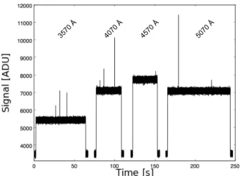
The data obtained from the photodiode, used to monitor the SCALA light level, consist of three parts: (1) a two second back-ground exposure; (2) a “light-on” exposure of variable length and (3) another two second background exposure. The two back-ground exposures, performed with the monochromator shutter closed, track the dark current of the photodiode and the back-ground ambient light, and their potential time variation.
As illustrated in Fig. 2, the calibrated photodiode continu-ously records data for each wavelength exposure, with a fre-quency set at 1 kHz. Laboratory tests were used to verify that the timescale for significant dark current variations is longer than the longest SCALA line exposure time, and that the dark current is smoothly varying. An average of the two background measure-ments is therefore a good estimate of the dark current that the photodiode experienced during the light exposure. This back-ground averaging method achieves a random error <0.2% for calibration of most wavelengths for nighttime photodiode data. The background subtraction procedure and its accuracy are fur-ther discussed in Sect. 7 and in K16, where daytime ambient light contamination is also discussed.
The shutter of the monochromator is the element ultimately determining the exposure time for each SCALA wavelength ob-servation. CLAP data are not only used as a light monitor but
3570 Å 4070 Å 4570 Å 5070 Å
Fig. 2.Example of the data obtained from one CLAP for a SNIFS blue-channel exposure. Notice the different exposure time for each wave-length, depending on the light level and SNIFS transmission, and also the presence of ∼2 s background exposures before and after observing each wavelength. The outliers in the data are cosmic rays, which are subsequently removed by the analysis software. The wavelengths ob-served are printed above the CLAP data for each exposure.
also as independent means to measure the exposure time, with a precision better then <0.01% for our shortest exposure times. With the 1 kHz sampling frequency of the CLAP, we are even able to measure the rising and falling ramp due to the opening and closure of the monochromator shutter.
4. System characterization
The calibration of the “telescope+ SNIFS” system requires a precise characterization of our instrument. We structured this in two steps: first the measurement of the response of each SCALA component individually in the lab, and second, the measure-ment of the fully integrated system. Consistency between the two approaches will verify that the SCALA output and moni-toring is understood at the component level. Any detected dif-ferences would focus attention on the types of changes that may need careful monitoring or remeasurement when using SCALA in situ. The two sets of measurements are detailed in Sects.4.1 and4.2, respectively. In Sect.4.3we discuss our ability to char-acterize the light output by SCALA, and how the light trans-mitted to the telescope by the 18 independent beams is scaled relative to the output of the beam monitored by the reference photodiode as function of wavelength.
4.1. Response of SCALA components
Laboratory measurements like those described in this section proved essential for selecting components able to produce con-sistency in the color output between the 18 SCALA beams. Good color uniformity is important because color differences between beams have the potential to introduce systematic errors if the reflectively of the primary mirror were also sufficiently non-uniform so as to reweight beams of different colors as seen by SNIFS.
Wavelength-relative throughput curves have been measured in a controlled laboratory environment for every single part of the system, including the mirrors, the ISs and the fiber bundle arms. These measurements used a monochromator and Xe lamp system separate from, but essentially identical to, the SCALA
monochromator and Xe lamp. Two lock-in amplifiers were used in combination with a chopper to amplify the signal received by model UV-035 EQC (not CLAP) monitoring and signal pho-todiodes. These measurements consist of ratios made using the same photodiode, at every wavelength, for both signal and mon-itoring systems and therefore the QEs of the photodiodes can-cel out. We kept the monitoring setup fixed when measuring each type of SCALA component. Since the small variations of the Xe lamp light level between measurements of the individual SCALA components are corrected by ratios of measurements made using the monitoring photodiode, the wavelength depen-dence of the component scanned by the monitoring setup also cancels out. The reference components (labeled as IS 1, Fiber 1 and Mirror 1, in Fig.3) were chosen to be those that were ulti-mately integrated to make the beam monitored by the reference CLAP when using SCALA in situ.
Our goal in the following sections is to compare the lab measurements with the commissioning measurements. However, the Xe lamp has bright emission lines longward of 7000 Å, and these are narrower than the resolution of the exit slit of the monochromator. These lines were found to cause too much vari-ability in the comparison between different sets of laboratory measurements since even tiny variations in wavelength repro-ducibility of the monochromator grating led to strong changes in the monochromator output. Therefore comparisons are pos-sible only below 7000 Å. The Xe lamp also has emission lines at 4500–5000 Å. However, as these lines are much weaker and introduce only modest added scatter (which we highlight in the relevant figures), the comparison data in this wavelength range can still be used.
4.1.1. Optical fibers
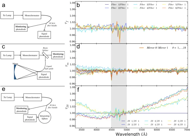
For the characterization of the optical fiber bundle arms, we im-plemented the measurements according to the setup shown in Fig.3a (upper left). The input end of the SCALA fiber bundle was mounted at the exit of the monochromator. Then the end des-ignated as the reference was monitored by the monitoring photo-diode while the signal photophoto-diode was used to measure the light from each of the remaining five fiber bundle arms. We cycled through the different fiber bundle arms until all five fiber bun-dle arms had been scanned in wavelength using a step of 30 Å. These relative responses are plotted in Fig.3b as τf. They have
been normalized at 5000 Å to aid in evaluating color trends. As can be seen, the fiber bundle arms are very similar, having rela-tive color trends smaller than 1%.
4.1.2. Mirrors
The reflectivities of the 18 mirrors were measured using the same lamp and monochromator system as above, but this time a beam splitter divided the light between the monitoring photodiode (al-ways the same) and the entrance of a liquid light guide. The exit of this guide illuminated a SCALA mirror, and the light was then focused on the other photodiode, as shown schemat-ically in Fig.3c. Each mirror was sequentially placed as shown in Fig. 3c and scanned in wavelength, without modifying the rest of the set-up. We scaled the signal photodiode measure-ments to the respective monitoring photodiode signal to correct for lamp variation between the individual measurements. In this way the wavelength trend of the unmodified part of the light path cancels out in the ratios. In Fig.3d we plot the ratios between the responses of the different mirrors with respect to that of the
Xe Lamp Monochromator Reference photodiode Signal photodiode SCALA fiber bundle Integrating Sphere
Xe Lamp Monochromator photodiodeReference
Signal photodiode Beam Splitter Mirror Liquid light guide Xe Lamp Monochromator Reference photodiode Signal photodiode SCALA fiber bundle Mirror #/ Mirror 1 # = 1,…,18 Monitoring Monitoring Monitoring Monitoring Monitoring Monitoring
a
c
e
b
d
f
Fig. 3.Left (panels a, c, e): set-up used in the laboratory to measure the corresponding quantities on the right side of the plot. Right (panels b, d, f): relative responses of the SCALA fibers (b), mirrors (d), ISs (f ), with respect to their reference component and normalized at 5000 Å for illustration purposes. The gray band delimits the region where the weak emission lines of the Xe lamp are located (4500–5000 Å).
reference mirror as τm, again, normalized at 5000 Å. The color
trend in these reflectivity comparisons is mostly gray, except for the shortest wavelengths where it is around 1%.
4.1.3. Integrating spheres
Finally, the integrating sphere responses were measured. We first mounted the input end of the SCALA fiber bundle at the exit of the monochromator. Then the end of one fiber bundle arm was connected to the IS entrance port and the signal photodi-ode was positioned immediately in front of one of the IS exit ports (Fig.3e). The monitoring photodiode was used to simulta-neously monitor the designated reference fiber bundle arm. For this series of measurements each IS was installed and measured in turn, without changing the rest of the set up. Care was taken to fix the IS positions with respect to the signal photodiode, and to not change any other elements, while cycling through each IS. In Fig.3f the responses of the integrating spheres, τIS, with
respect to one of them are shown, again normalized at 5000 Å. Here color trends of up to 8% are observed. This is likely due to the slight composition differences of the PTFE (Teflon) blocks from which they were machined. Fortunately, as we show in Sect.7.2, when we take this into account we see reproducible re-sults, and minimal systematic uncertainty from these chromatic differences.
4.2. Response of the fully integrated system
The second step of the SCALA system characterization is a mea-surement of the relative throughput, as a function of wavelength,
for each of the 18 beams in the assembled configuration. The precise characterization of the system can be ensured only if we know the behavior with wavelength of every SCALA beam.
4.2.1. Laboratory measurements
In the previous subsections we showed that all the relative re-sponses of SCALA components have different behaviors as functions of wavelength. The single component responses are now numerically combined to mimic the full system that was shown in Fig.1by calculating the quantity:
Pi, j,k(λ)= τfi(λ) · τISj(λ) · τmk(λ), (1)
where Pi, j,k(λ) is the relative response of one of the SCALA
beams when using the ith fiber bundle, jth integrating sphere and kth mirror, all taken with respect to the reference beam. The τ functions in Eq. (1) are those plotted on the right side of Fig.3, but in this case without normalization at 5000 Å. The sum over all 18 beams is used as an estimate of the total light expected to be produced by SCALA, and will be used in Sect.4.3.
4.2.2. In situ measurements
The light from SCALA as seen in the telescope focal plane con-sists of the sum of the flux reflected by the 18 mirrors. Now we show how to construct the analog of Eq. (1) for SCALA installed at the observatory. We express the wavelength dependence of the
SCALA light reproducibility, Es, as follows: Es(λc)= 1 + 18 X i=n=2 Ci(n)t (λc) · Dt(λc) Crn(λc) · Dr(λc) , (2)
where Cnr is the nth flux measurement by the reference CLAP
corresponding to the flux, Ci
t, measured by the test CLAP in the
ith beam for the SCALA line centered at λc. Dr and Dt are the
factors to convert the reference CLAP and the other CLAP mea-surements, respectively, from ADU to W, obtained by weighting the photodiode calibration curve – provided by the DICE team – by the SCALA line profile. Es is therefore the number of times
the light measured by the reference CLAP should be multiplied to represent the total SCALA output. If all beams were identical to the reference beam, Eswould be equal to 18 for every
wave-length. Here, we neglect the fraction of beam obscured by the photodiode as it is always obscured by the primary mirror mask. In order to measure the transmissions of all the beams for the in situ set-up we performed 17 independent sequences of SCALA monotonic scans in wavelength using one CLAP as ref-erence – always facing the same mirror – and manually moving the other CLAP from one mirror to another.
In order to reflect a collimated beam without being ob-structed by the IS, SCALA mirrors are mounted in an off-axis configuration. Due to this geometry, there is an illumination gra-dient across the reflected beam. This means that the sensitive area of the photodiode experiences a different amount of light depending on which part of the beam it samples. Thus, we took care to position a CLAP to always cover the same region of the SCALA beam that was being measured. We were able to achieve a reproducibility better than 0.7% in the wavelength range of interest (as will be shown in Sect. 7.3). Es has been measured
during the two commissioning phases in 2014 and 2015. 4.3. SCALA light reproducibility
The comparison between the three sets of measurements of the total light produced by SCALA provides two important pieces of information regarding our system: how well it is understood at the component level and its stability over time. This rests on comparing the calculated sum over the components of the 18 beams from Eq. (1) to the quantity in Eq. (2) measured in situ on the fully integrated system in 2014 and 2015.
4.3.1. Lab measurements vs. 2014 commissioning
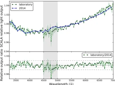
By selecting the appropriate IS, fiber bundle and mirror and by combining these 18 beam response functions according to Eq. (1), we can calculate the expected response of SCALA as fully integrated and operated at the telescope. The responses of ISs, mirrors and fiber bundles measured in the lab and plotted in Fig.3are each scaled by the respective IS, mirror or fiber bun-dle response of the reference beam, thus mimicking the in situ set-up wherein responses are measured relative to the reference CLAP. The sum over these 18 relative responses is shown with green squares in the top panel of Fig.4. This curve is compared with the 2014 measurements of the fully integrated system, as determined using Eq. (2) (blue circles). The measurements in this plot stop at 7000 Å since redward of this the laboratory tests used a Xe lamp whereas the in situ data used the halogen lamp. The measurements have been normalized to their average val-ues since we are only interested in comparing their color trend and not their absolute values. These averages are computed over
Fig. 4.Top panel: quantity Es. In green is the wavelength dependence of
the SCALA relative light output estimated from the laboratory measure-ments. In blue is that measured from the commissioning in May 2014. Both have been normalized with respect to their average to compare their color trend. Bottom panel: ratio between the laboratory measure-ment and the 2014 commissioning measuremeasure-ments. The dashed lines rep-resent the ±1% range around the averaged ratio of 1.000 (full line). The dotted lines are the measured standard deviation of 0.4%. The ver-tical gray band delimits the region where weak emission lines of the Xe lamp are located (4500–5000 Å). The measurements have been per-formed with the Xe lamp and therefore they only go up to 7000 Å.
the wavelength range shown in the plot, and equal 19.12 for the lab measurements and 18.95 for the 2014 in situ measure-ments. As can be seen in Fig. 4b, the ratio of the component-wise-combined measurements and the in situ measurements in 2014 does not show a color trend over the wavelength range where the two sets of measurements. The scatter in the ratio is 0.4%, which is within the expected errors (shown with a shad-owed area around the line). The color trend in the upper panel of Fig.4 is dominated by the relative transmissivity of the ISs, as shown in Fig.3and discussed in Sect.4.1.3. Those two mea-surements were separated by only 2 months, but in that time the system was shipped and reassembled. That it stayed so consis-tent is very impressive and encouraging. The agreement of the curves in Fig.4 together with the consideration that they have been measured with independent setups, proves that SCALA is a highly reproducible system (at least for the overlapping wave-length range). It also demonstrates the success of our method, whereby the wavelength behavior of the SCALA relative light output is reconstructed based on photodiode measurements taken with only two of the SCALA beams at any one time. From this we conclude that for SCALA we understand the per-component causes of the wavelength behavior, and can reproducibly mea-sure the system response.
4.3.2. Commissioning measurements in 2014 vs. 2015 By comparing in situ measurements taken over the year-long baseline between 2014 and 2015, we have detected a change in SCALA. Figure5 shows Es for 2014 (blue circles) and 2015
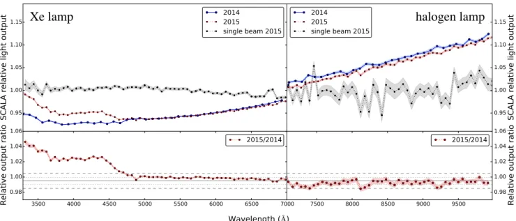
(red circles). A significant difference can be seen in the bluer wavelengths in the 2015 estimation (left panels). These curves are normalized with respect to their average values of 20.09 and 19.46 for the 2014 and 2015 measurements respectively, com-puted over the full wavelength range. The colored bands around
Xe lamp
halogen lamp
Fig. 5.The quantity Esis shown in the top panel for both figures, the SCALA relative light output from the commissioning in May 2014 is in
blue and the latest commissioning in May 2015 is in red. Both are normalized to their average values to compare only their color trend. One of the mirrors illuminated by the same IS as the reference for the 2015 SCALA relative efficiency measurements, normalized by its average value, is shown using solid black circles. Bottom panels: ratios between the two sets of commissioning measurements. The dashed lines represent the ±1% range around the averaged value computed for the measurements from 4700 Å to 10 000 Å, where a gray offset is present. The full line, around 0.995, is the average and the dotted lines span the standard deviation interval (±0.005). The quantities in the left panel refer to Esmeasured with
the Xe lamp while the right panel shows the measurements with the halogen lamp. the data points represent the statistical errors on the
measure-ments. They are larger on the right side of the plot due to the smaller statistics caused by the lower level of light produced by the halogen lamp. The coarser wavelength sampling of the curves in 2014 relative to 2015 is due to a reduced fraction of time devoted to the Es measurements. In 2015 we opted for a
more refined sampling and performed the measurements during three days.
One known difference is that the SCALA mirrors were cleaned before performing the measurements in 2015, and the reference mirror was cleaned more thoroughly compared to the others due to its easier accessibility. From this alone, a relative difference between the different beams and the reference beam is expected. Redward of 4700 Å the ratio between the responses for the two years is achromatic, and continues to be so beyond the lamp switch-over at 7020 Å (right panels of Fig.5). Over this wavelength range the overall mean ratio is 0.995 (full line) and the standard deviation of the ratio is 0.005 (dotted lines).
This change, at the blue wavelength end, might be due to a more accentuated degradation of the reference beam response with respect to the other beams. More specifically, a comparison between the responses of the two other beams belonging to the same IS as the reference beam do not show a deviation in the blue end, thereby excluding a relative degradation of the refer-ence CLAP with respect to the other CLAP. One of the beams illuminated by the same IS as the reference, normalized by its average value of 0.70, is plotted in Fig.5with solid black circles and the label “single beam 2015”. The fact that it is a smooth and mostly achromatic curve further suggests that the two CLAPs and the two mirrors did not degrade differently. Instead, a color trend appears when the other beams from the other five ISs and fiber bundle arms are included in the comparison (red curve in Fig.5). This suggests that the change occurred in the IS and/or fiber bundle arm of the reference beam with respect to the others. To explicitly test the reproducibility of our measurements, in 2015 we repeated the measurement of the relative responses of
one of the beams on the first and last days. The result of this test is discussed in Sect.7.3, where we find our measurements to be reproducible at wavelengths above 4700 Å, but that a 0.8% discrepancy exists blueward of this. This may be a partial con-tributor to the change seen between 2014 and 2015 for the bluest wavelengths shown in Fig.5.
Together, these results point to excellent reproducibility in the performance of SCALA redward of 4700 Å, and the need for further study of the behavior for the bluest 20% of the wave-length range.
5. “Telescope + SNIFS” calibration strategy
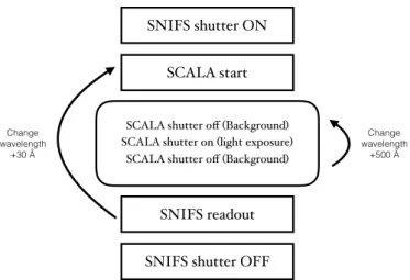
We now turn to the calibration of the telescope and instrument. A schematic example of the calibration strategy is shown in Fig.6. In this conceptual diagram the block that shows background and SCALA light exposures refers to measurements by the calibrated photodiodes, as previously discussed in Sect. 3. To minimize time spent on readout of the SNIFS CCDs, we observe SCALA at several well-spaced wavelengths per SNIFS exposure, using the monochromator shutter to control the exposure time for each wavelength. The SCALA line profile has a triangular shape with a FWHM of 35 Å. In K16 we verified that a separation of 500 Å between the wavelengths observed within one SNIFS exposure yields negligible cross-talk or overlap between adjacent wave-lengths or adjacent spaxels. Furthermore, we avoid crowded im-ages or long exposures, by limiting the maximum number of wavelengths per exposure to four for the blue channel calibra-tion (3300–5200 Å) and ten for the red (5000–10 000 Å). A typ-ical SNIFS exposure, after processing as in Sect.2.1, is shown in Fig.7 for an observation of SCALA by SNIFS in the blue channel. A SCALA observing sequence that calibrates the full SNIFS wavelengths range with a chosen wavelength sampling (from 30 Å on) therefore consists of multiple SNIFS exposures,
SNIFS shutter ON
SCALA start
SCALA shutter off (Background) SCALA shutter on (light exposure)
SCALA shutter off (Background)
Change wavelength
+500 Å
SNIFS readout
SNIFS shutter OFF
Change wavelength
+30 Å
Fig. 6.Data taking scheme for a full wavelength calibration scan with SCALA. The rounded SCALA box represents the measurements per-formed by the CLAPs, while the SNIFS boxes represent observations with the spectrograph. The arrows indicate the loops used to generate observations of multiple SCALA wavelengths per SNIFS exposure, and to interleave these exposures to obtain dense sampling in wavelength over the full optical range.
3570Å 4070Å 4570Å 5070Å
Fig. 7.Example of the wavelength-calibrated spectrum obtained from one of the spaxels of SNIFS for the blue channel. This is a typical ex-posure showing the 500 Å separation between the different wavelengths observed (the same as in Fig.2) and the nearly consistent number of electrons per wavelength due to a careful selection of the SCALA ex-posure time for each wavelength. The characteristic triangular shape and 35 Å FWHM of the SCALA line profile is also evident.
each containing four or ten monochromatic lines, depending on the SNIFS channel.
The exposure time for each wavelength observation was set such that the corresponding S /N > 100 per spaxel. The S/N depends on both the number of photoelectrons from the com-bined SCALA output beams, the telescope throughput, and the sensitivity of SNIFS at each wavelength. The resulting exposure times range from 30 s to 180 s. The overall time required for a complete “telescope+ SNIFS” calibration is 8 h. However, the flexibility of our acquisition software allows us to considerably reduce the exposure time for a calibration sequence, if desired. One can, for example, use larger wavelength steps within each SNIFS exposures, which offers the possibility to calibrate SNIFS more quickly. For example, calibration in steps of 150 Å can be
completed in less then 2 h. This option is very useful for test and commissioning runs, as well as for fast (and possibly daily) measurements of throughput.
6. Pilot observing run
During the 2015 commissioning, from June 3 to 7, we performed a series of SCALA measurements with SNIFS during night-time, using the newly-commissioned aperture mask. We alter-nated SCALA observations with standard star observations in order to check the stability of the “telescope+ SNIFS” calibra-tion from SCALA during the night. Due to non-photometric con-ditions and telescope issues, only the last night of observations, performed with an average seeing of 1.35 arcsec, was considered suitable for combining SCALA and standard star observations.
In the following subsections we detail our star/SCALA ob-servation strategy for this night (Sect.6.1) and show the resulting throughput measurement (Sect.6.2). Application of the SNIFS calibration to standard stars is on-going, so is not presented here.
6.1. Observation strategy
We subdivided the night into 5 sections. We initially performed a ∼2 h SCALA calibration sequence, starting from 3330 Å with steps of 180 Å, during evening twilight, when the influence of ambient light in the dome is small compared to full daytime light. Then we opened the dome and performed standard star ob-servations for ∼2 h. We closed the telescope dome and performed another SCALA calibration sequence with the same steps, but this time starting at 3390 Å. We resumed observing stars until the end of the night, and finally took a SCALA calibration sequence in the morning starting at 3450 Å. To ascertain the stability of the overall system during the night, e.g. SCALA alignment with the telescope and the “telescope+ SNIFS” throughput, a sub-set of nine wavelengths was reobserved during all three SCALA blocks during the night. We denote these monitoring sets of ob-servations as A, B and C.
Combining the SCALA calibration sequences performed during the night, provides us with 111 measurements of the in-strumental response giving a complete SNIFS calibration sam-pled at 60 Å intervals. The system stability can be examined by computing the ratios between the throughput of the reobserved wavelengths, A/B and C/B. From 4000 to 9000 Å, these two ra-tios are consistent with each other and centered around 1.001 with standard deviation of 0.003 (see Sect. 7.9). In the 3300– 4000 Å region, the morning run (C) shows a 2% offset. Note that these are upper limits to the system stability as the A surements were performed during evening twilight, the B mea-surements during night and the C meamea-surements were performed after sunrise in the morning. This results in different levels of ambient light in the dome, for which the software corrects using the CLAP background data segments, as shown in Fig.2.
6.2. Throughput measurement
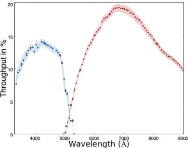
The throughput measurement is accomplished by comparing the observations of SCALA by SNIFS against those from the calibrated reference photodiode, according to the following equation: T(λc, spx) = R ISNIFS(λ, spx)E0(λ)dλ Cr(λc) · Dr(λc) · G Es(λc) , (3)
Fig. 8.Nighttime throughput, Tλi,spx, of the telescope plus SNIFS,
av-eraged over all SNIFS spaxels. The blue and red circles represent the throughput measured by illuminating the blue and red spectroscopic channels, respectively, and the telescope with SCALA. The colored bands indicate the throughput standard deviation between SNIFS spax-els, and are thus not an estimate of the throughput uncertainty.
where ISNIFS(λ, spx) is the SCALA line intensity centered at λc
observed by SNIFS in each spaxel, spx, in electrons and E0(λ) is the energy of the photon for the wavelength λ; Cr is the
inte-grated light measured by the reference CLAP (over the SCALA line exposure time); Dr is the factor to convert the reference
CLAP measurement from ADU to W, as in Eq. (2); Es(λc) is
the SCALA light output relative to the reference CLAP from the 2015 measurements as in Eq. (2) and shown in Fig.5 (with-out normalization this time); G is the geometrical factor that accounts for the different dimensions of the CLAP and SNIFS and also their different fields of view. The geometrical factor, G, is determined by multiplying the ratio of areas of the CLAP (5.8 × 5.8 mm) versus area of a SCALA mirror against the ra-tio of the solid angles of the SCALA beam (1◦) versus that of
a SNIFS spaxel. Once scaled for the SCALA mirror and CLAP area, the factor Cr(λc) · Dr(λc) · Es(λc) provides the total
illumi-nation generated by SCALA as function of wavelength.
From the average of Eq. (3) over all spaxels we obtain the mean throughput curve shown in Fig. 8. This curve has been measured by combining the three blocks of SCALA calibra-tion sequences performed during the same night, as explained in Sect.6.1.
Application of this throughput measurement to the computa-tion of the flux of a standard star is straightforward. The SNIFS optics reimage the telescope pupil onto the detector, thus, the fluxes from SCALA or from a standard star are extracted from the CCD detectors in an identical fashion when building a dat-acube. The datacube from SCALA is then used to flux-calibrate each wavelength of each microlens in the datacubes of standard stars; that is, it provides a surface-brightness calibration. The fi-nal reported stellar flux for each wavelength results from a point spread function (PSF) fit over the 6.400× 6.400 spatial extent of
the microlens array. For typical seeing experienced with SNIFS on Mauna Kea, the microlens array contains more than 99% of the light comprising the PSF model (Buton 2009). Therefore, the portion of the flux based on extrapolation of the PSF is quite small.
7. Systematics
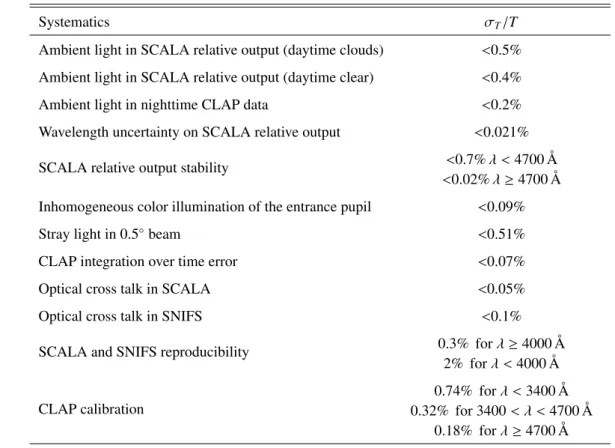
In this section we carefully examine the various sources of un-certainty. Some may be statistical, such as the repeatability blue-ward of 4700 Å, but we include them as systematics until more is known. The known or potential sources of systematic uncer-tainty are summarized in Table2. Some of these errors are cor-related because they are based on the same sets of calibration measurements and thus their statistical errors will be strongly correlated. Counting the statistical errors more than once would be incorrect. Thus, the net systematic uncertainty will be much less than the quadrature sum of the values listed in Table2. The full covariance matrix, required for the final calibration, will be presented by Küsters et al. (in prep.).
Of the measurements composing Eq. (3), the biggest con-tribution to the uncertainty is due to the Es. This particular set
of measurements has been performed under rather different con-ditions than the observations of SCALA by SNIFS, making it subject to several sources of contamination:
– since these measurements were made during daytime, they can have residual ambient light contamination (see Sect.7.1);
– since these measurements do not have associated SNIFS observations to provide precise wavelength measurements, we need to consider the uncertainty caused by the limit re-producibility of the monochromator wavelength setting (see Sect.7.2);
– reproducibility of the photodiode position for each mirror when cross-calibrating each beam (Sect.7.3).
In the following we start with these systematics, both for the nighttime and daytime measurements, and then consider the sys-tematics related to the other elements of Eq. (3). We also note that Esmeasurements have higher statistical uncertainties due to
their shorter exposure times.
7.1. Ambient light contamination
The throughput measurements derived using Eq. (3) were per-formed mostly during nighttime with the telescope dome closed. Ambient light contamination can, therefore, be neglected in the analysis of the calibrated photodiode data. On the other hand, Es
was measured during daytime and, therefore, dome light leaks could lead to varying levels of ambient light contamination.
During the day there are two cases that can occur: diffuse and scattered ambient light that smoothly drifts with time, and scat-tered ambient light that quickly varies on a timescale of seconds, e.g. due to clouds crossing the sky. Variations on timescales longer than individual SCALA line exposures can be accurately accounted for by interpolating the CLAP background measure-ments. For these cases the background measurements before and after the light exposure (Fig.2) are representative of the dark current and ambient light level during the light exposure.
The partly-cloudy daytime case is more complicated. To es-timate the uncertainty on background removal we have obtained a series of daytime (and nighttime) CLAP measurements with only ambient light, as shown in K16. We tested the precision of the background reconstruction by artificially dividing these data into background and signal segments, and measuring how well we retrieve the background. From such tests we find that a sim-ple linear interpolation of the background shows good results, with a reconstruction of high-frequency background variations
Table 2. Systematic uncertainties that contribute to the total uncertainty on the throughput measurements.
Systematics σT/T
Ambient light in SCALA relative output (daytime clouds) <0.5% Ambient light in SCALA relative output (daytime clear) <0.4%
Ambient light in nighttime CLAP data <0.2%
Wavelength uncertainty on SCALA relative output <0.021%
SCALA relative output stability <0.7% λ < 4700 Å
<0.02% λ ≥ 4700 Å Inhomogeneous color illumination of the entrance pupil <0.09%
Stray light in 0.5◦beam <0.51%
CLAP integration over time error <0.07%
Optical cross talk in SCALA <0.05%
Optical cross talk in SNIFS <0.1%
SCALA and SNIFS reproducibility 0.3% for λ ≥ 4000 Å
2% for λ < 4000 Å
CLAP calibration
0.74% for λ < 3400 Å 0.32% for 3400 < λ < 4700 Å
0.18% for λ ≥ 4700 Å
that is better than 6% of the faintest (longest exposure) line emit-ted by SCALA. However, as the Esdetermination relies on ratios
between simultaneous measurements from two different CLAPs and the background misestimates are strongly correlated, the er-ror on the signal ratio reconstruction is mostly compensated. The net error is of order of 0.5%.
Datasets for only a few mirrors exhibit such fast variations during periods when Esλi was being measured in 2015.
In K16 we showed that for diffuse and scattered ambient light that smoothly drifts with time, the background misestimate of the SCALA relative light output is less than 0.4% of the faintest line emitted by SCALA. As already mentioned, ambient light is not a concern during nighttime measurements, where CLAP dark current variations can be reconstructed to better than 0.2% of the faintest (longest exposure) line emitted by SCALA.
A possible way to further suppress this contamination, whether measurements are made during the day or night, would be to perform the SCALA wavelengths observations with ad-ditional background samples introduced during the light expo-sure meaexpo-surements. That is, closing the monochromator shutter during the light exposure would give a better sampling of pos-sible changes in ambient light, especially for long exposures. This would not increase the exposure times needed by SNIFS by much. By increasing the sampling frequency of the photodi-ode data, a constant statistical uncertainty could be maintained, as the error would be computed on a larger sample.
7.2. Wavelength uncertainty
Our calibration device produces monochromatic light through a monochromator, for which the stated wavelength reproducibil-ity is about 1 Å according to the manufacturer. For the SNIFS system throughput estimation we use the wavelength calibration
from SNIFS data to evaluate the central wavelengths observed, therefore this error does not directly appear in the systematics budget. It is present, though, in the determination of SCALA relative light output, Es, since in this case, to save time, we do
not obtain any associated SNIFS exposures.
We have used the SNIFS wavelengths calibration to ver-ify the stated wavelength precision by comparing the central SCALA wavelengths measured from a set of SNIFS exposures with those requested of the monochromator and recorded in the headers of the CLAP photodiode data. These follow a linear trend, which can be fit for the blue and red wavelengths as shown in Fig.9(panels a and d) together with their residuals (panels b and e). We find a residual trend after subtracting the linear fit to the data, with standard deviations of 1.51 and 1.01 Å for the blue and red channels, respectively. Under the assumption that the deviations are due to a stable mechanical effect, monochro-mator wavelength errors can be decreased further by subtracting the 20-point running average of the residuals. The standard devi-ation of these residuals is 1.39 Å, for the blue channel (Fig.9c), and 0.79 Å, for the red channel (Fig.9f). These reductions in the standard deviations have high statistical significance, so are not simply the results of random scatter. This combination of linear fits and running averages for the spectroscopic channel is used to fine-tune the monochromator wavelength in the determination of Es.
Such small errors in the wavelength estimates do not consti-tute an issue for the Esmeasurement. When recomputing Es
us-ing a wavelength that is artificially increased (or decreased) by one standard deviation, we find the same result within 0.021% (in the worst case).
Finally, we have compared multiple observations when the same wavelength was requested to the monochromator. These
R esi du al s - ru nn in g ave ra ge R esi du al s
Blue
a b c R esi du al s - ru nn in g ave ra ge R esi du al sRed
d e fFig. 9.Wavelengths measured using the SNIFS exposures for the blue channel (panel a) and the red channel (panel d) versus the ones re-quested to the monochromator, plotted together with the linear fit (black line). Panels b and e: residuals from the linear fits (blue squares) and running average of the residuals (red line), computed with an averaging window of 20 data points. The blue shaded region represents the stan-dard deviation interval of the data of ±1.51 Å (in panel b) and ±1.01 Å (in panel e). Panels c and f : results of subtracting the running averages from the residuals of the linear fits (blue squares). The blue shaded re-gion represents the standard deviation interval of the data of ±1.39 Å (in panel c) and ±0.79 Å (in panel f ).
are consistent with the monochromator wavelength reproducibil-ity stated by the manufacturer.
7.3. SCALA relative light output stability
We have tested the reproducibility of the SCALA relative light output, Es, by repeating the measurement of one of the
Fig. 10. Ratio, α/β, between repeated measurements of the same
SCALA beam is shown as black circles. The black line represents the average of 0.999 and the shaded gray region brackets the standard de-viation interval of ±0.8%. The vertical dashed line separates the data above and below 4700 Å. Redward of this the repeated measurements are highly reproducible, but blueward of this there are clear variations.
18 SCALA beams at the start and end of the four day calibration run. We denote these sets of CLAP ratios between the moving and reference photodiodes as α and β, respectively. The mean reproducibility is excellent, having a mean of 0.999 (blue line in Fig.10) and a standard deviation of 0.008. The measurements at the reddest wavelength range are noisier only because they have lower flux levels. These fluctuations are further suppressed when all 17 beams are combined. In regular nighttime observation we expose longer for wavelengths with lower intensity emission, and this maintains a constant S/N. When measuring the SCALA relative light output, such long exposure times are not feasible as the measurement has to be made 18 times (once for each non-reference beam+ the reproducibility sequence). For this test we used a constant exposure time of 5 s per wavelength.
As can be seen in Fig. 10, the ratio between sets α and β shows a 0.8% difference for blue wavelengths (<4700 Å), likely due to a change in the system on timescales of a few days. Rel-ative evolution of the IS and/or fiber bundle arm belonging to the reference projector module with respect to the other SCALA modules, as mentioned in Sect.4.3.2, is a possible cause. Mea-surements of the beams from the same reference module do not show this evolution, as visible from the plot of one of them in Fig. 5. Note that SCALA relative light output measurements were performed in a mixed order – not module by module – and the reference module beams were measured during the sec-ond day. To compute the contribution to the systematic error, we assume that this change is bracketed by the ratio of α to β, as β was the final measurement made and the nighttime measure-ments (for which we use the SCALA light output) were acquired just before the α data-set.
This systematic error is propagated to each of the SCALA beam measurements, except for the two beams that belong to the reference module and thus are illuminated by the same fiber bundle arm and IS. As each beam ratio has a similar amplitude, the total error on the SCALA relative light output is of the same order as the one from a single beam, <0.7%.