HAL Id: tel-02418618
https://tel.archives-ouvertes.fr/tel-02418618
Submitted on 19 Dec 2019
HAL is a multi-disciplinary open access archive for the deposit and dissemination of sci-entific research documents, whether they are pub-lished or not. The documents may come from teaching and research institutions in France or abroad, or from public or private research centers.
L’archive ouverte pluridisciplinaire HAL, est destinée au dépôt et à la diffusion de documents scientifiques de niveau recherche, publiés ou non, émanant des établissements d’enseignement et de recherche français ou étrangers, des laboratoires publics ou privés.
methodologies for trace elements pollution assessment in
different compartments of the marine environment
Anna Maria Orani
To cite this version:
Anna Maria Orani. Development and application of analytical methodologies for trace elements pollution assessment in different compartments of the marine environment. Other. Université Côte d’Azur, 2017. English. �NNT : 2017AZUR4112�. �tel-02418618�
ÉCOLE DOCTORALE SCIENCE FONDAMENTALES APPLIQUEÉS
Géoazur UMR 7329
Thèse de doctorat
Présentée en vue de l’obtention du
grade de docteur en Chimie
de L’UNIVERSITÉ COTE D’AZUR
par
Anna Maria ORANI
Développements analytiques pour la détermination des
concentrations et de l’origine des contaminants
inorganiques dans des environnements marins
Dirigée par Pr. Olivier THOMAS
et codirigée par Dr. Emilia VASSILEVA et Dr. Aurélie BARATS
Soutenue le 15 Décembre 2017 Devant le jury composé de :
Dr. Aurélie BARATS, Maître de conférences, Géoazur, Université Côte d’Azur co-directrice de thèse Prof. Ewa BULSKA, Chemistry Department, University of Warsow rapporteur
Prof. Veselin J. KMETOV, Analytical Chemistry Department, University of Plovdiv rapporteur
Prof. Christophe RENAC, Géoazur, Université Côte d’Azur examinateur, président du jury Prof. Olivier P. THOMAS, National University of Ireland Galway directeur de thèse
Development and application of analytical
methodologies for trace elements pollution assessment
in different compartments of the marine environment
AKNOWLEDGMENTS
First of all I would like to express my gratitude to Prof. Ewa Bulska, Prof. Veselin Kmetov, and Prof. Christophe Renac for their interest in my PhD work and for taking the time to review my thesis. I am confident that their suggestions will be of great help for my future.
This PhD comes to an end after a tortuous path, full of challenges but most importantly full of interesting experiences. A real life-changing adventure during which I have learnt a lot!
Many people helped me in this period, fighting for and with me and for this reason I will be forever grateful to each of them, starting from my supervisors:
-My PhD director Olivier Thomas, who accepted this role and never gave up even in the middle of many administrative challenges!
-My PhD co-director Emilia Vassileva, who encouraged me to start a PhD in the first place and with her precious teaching always supported my work and believed in me.
-My second PhD co-director Aurélie Barats, who helped and encouraged me even during the most difficult periods, with many advices and positive attitude.
Special thanks go to Prof Petko Mandjukov and Dr Irena Wysocka, for sharing their knowledge with me and for their crucial contribution to this PhD work and to Ms Sabine Azemard for her constant help. I would like to thank all the fellows and office mates I have been the pleasure to work with, in France and Ireland, which have contributed to accumulate many wonderful memories!
Je voudrais remercier toute la famille Calabro, pour m’avoir accueilli à bras ouverts ces dernières années et pour être toujours un gros point de référence, ma deuxième famille !
Ancora una volta vorrei ringraziare la mia meravigliosa famiglia e le mie fantastiche amiche che mi sono stati vicino (da lontano). Il loro sostegno è stato fondamentale in questi anni, e lo sarà per sempre. Voglio dedicare questa tesi a Kevin, che mi ha supportato (e sopportato) in questi anni, garantendomi amore incondizionato, condividendo con me le tante soddisfazioni ma soprattutto insegnandomi a non mollare e perseverare sempre!
PART I: GENERAL INTRODUCTION ... 11
1. Trace elements in the environment... 13
1.1. Trace elements in the aquatic system ... 13
1.2. Trace elements speciation ... 16
1.2.1. Arsenic ... 17
1.2.2. Mercury ... 20
1.3. Trace elements isotopes ... 22
1.3.1. Pb Isotopic ratios ... 24
2. Trace elements monitoring programs ... 26
2.1. Trace elements in sediments ... 27
2.1.1. Sediment components and classification ... 27
2.1.2. Factors affecting TE accumulation in sediments ... 29
2.1.3. TE monitoring in sediments ... 32
2.2. Trace elements in marine organisms ... 33
2.2.1. Bivalves ... 33
2.2.2. Sponges ... 35
3. Trace elements analysis ... 38
3.1. Atomic Absorption Spectrometry ... 40
3.2. Inductively Coupled Plasma Mass Spectrometry ... 41
REFERENCES ... 44
PART II: SCIENTIFIC PUBLICATIONS ... 69
FIRST BLOCK ... 71 Paper 1 ... 71 Paper 2 ... 81 Paper 3 ... 95 SECOND BLOCK ... 115 Paper 4 ... 115 Paper 5 ... 150 THIRD BLOCK ... 201 Paper 6 ... 201 Paper 7 ... 254
PART I: GENERAL INTRODUCTION
In this first part of the thesis, some general information is discussed. These concepts are useful for the
understanding of the general picture presented in this PhD.
The origin and fate of TE in different compartments of the aquatic system are presented as well as a
1. TRACE ELEMENTS IN THE ENVIRONMENT
The IUPAC Compendium of Chemical Terminology defines trace element as “any element having an average concentration of less than about 100 parts per million atoms or less than 100 µg g-1’’ (McNaught
and Wilkinson, 1997). Among TE, some are oligo elements and are thus considered essential for various biochemical and physiological functions within a certain range of concentrations. Metals/metalloids considered by World Health Organization to be essential for human health are: chromium, cobalt, copper, iron, molybdenum, selenium and zinc (WHO, 1996)(WHO, 1996).On the other hand, other TE are considered toxic at any concentration (Hg, Pb, Cd) (WHO/FAO/IAEA, 1996).
These elements are naturally present in the ecosystem because of natural processes such as weathering and erosion but also volcanic activity. Nevertheless, in the last decades, several anthropogenic activities have increased the loads of these elements in the environment (Bagul, 2015). Main anthropogenic sources of TE include metal mining, mineral processing, smelting, coal mining, power generation but also municipal waste incinerators, industrial waste of many types and petroleum utilization. Specifically, in coastal systems, the anthropogenic sources can be represented by building of infrastructure, land reclamation for port and industrial development, habitat modification, tourism and recreational activities (Rao et al., 2006). The levels of TE in the environment are thus dominated by several concomitant processes, related to the origin but also to the different fates of these components in through environmental compartments.
1.1.
Trace elements in the aquatic system
Trace elements have been transported along the hydrological cycle since the first occurrence of water on the planet. Water provides the medium for weathering of the continents as well as the medium for transport them in other environmental compartments (Salomons and Förstner, 1984). Along the way to the oceans, trace elements undergo different processes, due to environmental changes that affect their distribution in dissolved and particulate phases. TE under the form of particulates may accumulate in rivers and lakes and from there reach the coast through estuarine systems. Several important processes take place in the interfaces river/ocean as well as in the continental shelf. In these areas (often hosting harbors and industrial centers), TE from natural and anthropogenic origins are accumulated. Once the riverine or atmospheric TE loads have entered the oceans, they take part in an intricate group of geochemical processes, ultimately ending their path as
accumulated substance by marine sediments. An illustration of these complex patterns is shown in figure 1. The residence time of TE in aquatic environment varies from a few days (rivers and atmosphere) to several thousands of years (oceans) (Salomons and Förstner, 1984).
Figure 1. Movement of trace metals in the hydrological cycle. Copyright Springer
Intrinsic water characteristics such as physiochemical and biological properties have a great influence on the geochemical cycle of elements in the oceans (Elderfield, 2003). Trace elements can be found in the environment under the form of free cations (Mn+), which is the most bioavailable form
especially for aquatic organisms such as phytoplankton (Bruland and Lohan, 2003). Others are more often under the form of oxyanions, such as MoO42- and AsO42-. In aquatic ecosystems, trace elements are
very often bound to ligands. Most natural waters have a certain capacity to reduce the bioavailability, and thus the toxicity, of such elements, due to the presence of ligands complexing the free ions (Salomons and Förstner, 1984). Nevertheless, some of the complexes can, in turn, be bio-available, such as those accumulated by the marine biota (Vicente-Martorell et al., 2009; Strady et al., 2011). Water contamination can thus have a direct effect on the food chain as well as be biomagnified through it (Bocher et al., 2003; Majer et al., 2014). The understanding of TE cycle in the aquatic system is of prime
interest to address the right correction actions and help decision makers in the process of efficient restoration of natural conditions.
The behavior of trace elements in the water column is governed by several factors. Direct precipitation of dissolved elements is possible as a consequence of changes in physiochemical condition, such as pH, oxidation potential or concentrations of precipitating substances. These circumstances can occur as a consequence of water mixing processes, loss or addition of gasses as well as the mixing of water with solids (Rose and Hawkes, 1979). An example is the precipitation of U, V, Cu, Se, and Ag as metal or lower-valency oxide because of reduction usually caused by an encounter with organic matter or mixing with reducing waters or gases. The redox potential Eh thus plays a crucial role in the behavior
of trace elements in aquatic environments. In natural system, Eh is often a measure of total dissolved
oxygen, although other dissolved species can act as oxidizing (NO3-, SO42-) and reducing (Fe2+, Mn2+)
agents (Plant and Raiswell, 1983). The pH also influences the mineral dissolution and precipitation reactions, additionally affecting the complexing process. The speciation of many elements in the surface environment may be represented in Eh vs pH diagrams (Plant and Raiswell, 1983). An example is shown
in Figure 2.
Figure 2. Potential-pH diagram for Cu in water. Full lines separate the stability fields for copper species. The y-axis is the potential in Volts with respect to hydrogen electrode (Nolan and Cadien, 2012)
TE occurrence of TE in the particulate or dissolved phase of water affects directly their assimilation by organisms and thus their involvement in marine biogeochemical cycles. Additionally, their solubility is influenced by their source, so the way through which they reach the water column. For example, trace
elements having an urban source are more soluble than those derived from crustal weathering (Chester et al., 1993). It is possible to distinguish three main groups on trace elements, depending on their behavior all along the water column, as shown in Figure 3 (Bruland and Lohan, 2003):
• Conservative (or bio-unlimited) elements: low affinity with particles and long residence time; their concentration does not change with depth (e.g., Cs, Rb, Mg)
• Nutrient elements: show lower concentration on the surface and higher in the bottom of water columns, as a result of plankton uptake and incorporation on the surface (e.g., Cd, Cr, Cu, Ag, As, Ba, etc.)
• Scavenged elements: have a high affinity for particles and they are rapidly sorbed onto particles and liberated to the sediments. Therefore, their concentration is lower in the bottom of water column
Figure.3. Classification of major and trace elements according to their behavior in the water column (adapted from Nozaki, 2001)
1.2.
Trace elements speciation
As already mentioned, trace elements can have variable toxicity which often depends on their chemical forms. As a consequence, the bulk concentration of the element is often not sufficient information for the assessment of its real toxicity (Chai et al., 2004). Consequently, in the last decades,
researches have been focusing on the analysis of chemical species of several TE to evaluate their impact on the environment (Sánchez Uría, 1998; Leermakers et al., 2005; Semeniuk et al., 2016). Among toxic elements, arsenic and mercury are two of the most studied elements regarding chemical speciation in environmental samples.
1.2.1. Arsenic
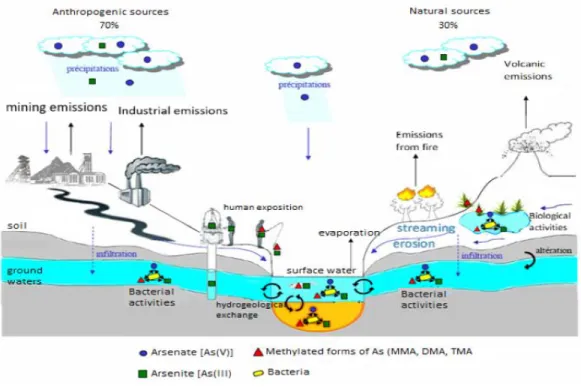
Arsenic (As) is classified as metalloid as it presents characteristics of both, metallic and non-metallic element (Phillips, 1990). It is associated with igneous and sedimentary rocks, particularly with sulfidic ores as it is strongly chalcophile. Several anthropogenic activities such as metals and alloys manufacturing, petroleum refining and burning of wastes and fossil fuels, have contributed to a strong legacy of As pollution throughout the world (Melamed, 2005). Several As-containing compounds are produced by industry and have been used to manufacture products for agricultural applications such as insecticides, herbicides, and fungicides. Numerous species of As can occur in the environment and the interconversion of species from toxic to less harmful and vice versa is possible as a consequence of some physical-chemical changes such as biological activity, changes in redox potential, or pH. To determine the actual risk represented by this element in the environment, a proper study should include identifying and quantifying both the total quantity of arsenic and the specific chemical forms present in the sample (Gong, 2002).
Figure 4. Structures of the principal As compounds in the marine environment (Leermakers et al., 2006)
In the environment, arsenic occurs usually under inorganic species, and rarely under organic ones (Figure 4). The main inorganic species are found under two oxidation states: arsenite As(+III) and arsenate As(+V), as the oxyacids (H3AsO3 and H3AsO4). In many environments (under neutral conditions),
As(+V) is often deprotonated as an arsenate oxyanion (H2AsO4- or HAsO42-); in contrast, As(+III) remains
predominantly in its neutral form as H3AsO3. Arsenate oxyanions and the neutral arsenite constitute the
main targets for field analytical assays (Melamed, 2005). Inorganic As species are found in water and soils and in small quantities in living organisms where rather organoarsenic species dominate. Some biological processes (mainly due to bacterial activities) can also promote the oxidation or the reduction of inorganic As (Anderson et al., 1992; Santini et al., 2004; Silver and Phung, 2005; van den Hoven and Santini, 2004). Usually freshwaters and ground waters scarcely contain organic As species such as methylarsonate (MMA, CH3AsO3H2) and dimethylarsinate (DMA, (CH3)2AsO2H) (Bednar et al., 2004;
Bohari et al., 2001; Martinez-Bravo et al., 2001). Organic As species (methylated species and arsenosugars) usually occur in biological organisms (particularly in marine ecosystems). Arsenobetaine (AsB) is usually the dominant As species occurring in fishes and seafood, but other methylated
compounds are also found in marine biota (Nam et al., 2010; Grotti et al., 2010). Biological processes promoted by some microorganisms or bacteria enhance the methylation of inorganic species in organic ones, such as MMA, DMA, trimethylarsine [TMA, (CH3)3As] (Bentley and Chasteen, 2002; Cullen and
Reimer, 1989; Irgolic and Stockton, 1987). Arsenic is essential for some organisms, e.g., 12 to 25 μg of total As per day is required by humans, but it is also toxic at low and high concentration (WHO, 2006). Chronic As exposure increases the risk of cancer and skin pigmentation. Arsenic has great notoriety as a poison, though there are great differences in the toxicity of different arsenic compounds. Arsenic occurs as organic and inorganic species, and it can have different oxidation states (-III, 0, +III and +V). Its toxicity also depends on its valence and speciation, inorganic species being by far the most toxic species (Table 1).
Table 1. Experimental LD50 (median lethal dose) for some As compounds (adapted from Leermakers et al., 2006 and Levy, 1946) Arsenic species LD50 (g/kg) Arsine (AsH3) 0.003 Arsenite As(+III) 0.014 Arsenate As(+V) 0.020 TeMA 0.89 DMA 1.2 MMA 1.8 Arsenocholine >6.5 TMAO 10.6 Arsenobetaine >10.0
Most cases of arsenic human toxicity have been associated with exposure to inorganic arsenic. Inorganic trivalent arsenite As(+III) is 2–10 times more toxic than inorganic pentavalent arsenate As(+V) (Goyer, 2001). By binding to thiol or sulfhydryl groups on proteins, As(+III) can inactivate over 200 enzymes. This mechanisms is the likely mechanism responsible for arsenic’s widespread effects on different organ systems (Tchounwou et al., 2012). The acute toxicity of As(+V) is related to its ability to replace phosphate, which is involved in many biochemical pathways (Goyer, 2001; Hughes, 2002). Arsenic toxicity is much higher in inorganic forms than organic species of arsenic (Table 1). The major metabolic pathway for inorganic arsenic in humans is methylation. Most of the mammalian species methylate inorganic arsenic (Vahter, 1994). Inorganic arsenic is metabolized by a sequential process involving a two-electron reduction of inorganic pentavalent arsenic to inorganic trivalent arsenic, followed by oxidative methylation to pentavalent organic arsenic (Thomas et al., 2001). The reduction can occur non-enzymatically in the presence of a thiol such as glutathione (GSH) (Delnomdedieu et al.,
1994; Scott et al., 1993). However in human livers, some specific enzymes have been isolated, suggesting that the reduction occurs using enzymatic reaction (Radabaugh and Aposhian, 2000; Zakharyan et al., 2001). The species produced as a result of these reactions are then expelled along with urine.
Biogeochemical processes regulating As speciation is the aquatic environment are summarized in Figure 5. Biological activities, weathering, and volcanic activities on one hand and anthropogenic activities on the other, are responsible for the emission of inorganic As into the atmosphere, from where it is redistributed on the earth’s surface by rain and dry fallout (Cullen and Reimer, 1989).
Figure 5. Global arsenic geo-cycle (Bossy, 2010). Black and blue arrows represent arsenic emissions in the atmosphere and its entrance back in surface/ground waters
1.2.2. Mercury
Mercury (Hg) is non-essential and highly toxic trace element. This metal has a very different chemistry from its group and period neighbors, and it is the only metal liquid at room temperature. Mercury naturally occurs in the environment although it is considered rather rare chalcophile element. The principal mineral is cinnabar (HgS), along with the metacinnabar group of minerals; other primary
Hg minerals include native mercury, corderoite Hg3S2Cl2 and livingstonite HgSb4S8. Most mercury is
derived by natural sources but its biogeochemical cycles is disrupted by anthropic inputs as several human activities have contribute to increase its environmental input since the industrial revolution (Wu et al., 2006; Chen et al., 2013; Lamborg et al., 2014). Anthropogenic sources of mercury come from metal production, chlor-alkali, and pulp industries, waste handling and treatment, and coal, peat, and wood burning (Lindqvist et al., 1991).
Mercury occurs in the environment under three principal forms: Hg(0), inorganic Hg and organic forms such as methyl mercury (MeHg). Hg coming from natural and anthropogenic sources is principally emitted in the atmosphere, where its global cycle (Figure 6) is largely controlled by oxidation–reduction reactions. For instance, it can easily oxidize into soluble (inorganic) Hg2+ which in turn can deposit on
water and soil surfaces. A small fraction of mercury in natural waters is converted to organic forms such as methylmercury (CH3Hg+) and dimethylmercury [(CH3)2Hg], by bacterial action in anoxic environments.
Metallic Hg is relatively inert and not readily taken up by organisms, but it is volatile and its vapor is toxic. Inorganic forms such as HgCl2 are also considered toxic especially for long-term exposure (Lohren
et al., 2015). Fat-soluble organic forms (especially MeHg) accumulate in the biota via the food chain (up to several mg kg-1), resulting in human exposure through consumption of fish (Morel et al., 1998). This
compound is considered the most toxic form of mercury since it causes serious central nervous system dysfunctions (Harada, 1995). Additionally, contrary to other trace elements efficiently accumulated by organisms, Hg is bio-magnified through the food chain, meaning that the highest concentrations of this element are found in the highest levels of the food chain. Hg(0) and Me2Hg are not bioaccumulated by
organisms because they are not reactive and thus not retained by plankton in the first place (Morel et al., 1998). On the other hand, Hg(II) is efficiently retained by microorganisms but not efficiently transferred to other organisms through food chain in comparison to MeHg (Mason et al., 1996) as it probably happens when considering other trace elements. In 2013, a multilateral environmental agreement known as Minamata convention, has been promoted by UNEP and it addresses the adverse effects of mercury through practical actions to protect human health and the environment from anthropogenic emissions and releases of mercury and its compounds (Briant et al., 2017).
Figure 6. Mercury cycling and methylation in the aquatic environment. (Morel et al., 1998). SRB stands for Sulfate Reducting Bacteria. MerA and MerB are enzymes involved in the hydrolysis of MeHg and reduction of Hg(II) respectively (Morel et al.,
1998)
1.3.
Trace elements isotopes
Many elements exist in nature with different isotopes, i.e., atoms of the same element which differ from each other only in their number of neutrons. Generally speaking, it can be stated that all elements have an isotopic composition stable in nature. However, there are some reasons why this isotopic composition may show some variation. One of this reason is the presence, among the isotopes, of radiogenic nuclides. Such nuclides are produced as a result of radioactive decay. The additional production of this radiogenic isotope can have a pronounced effect on the final isotopic composition of a given element. Other phenomena responsible for a change in isotopic composition are interaction with cosmic rays, mass-dependent and mass-independent mass fractionation and the presence of extraterrestrial material (Vanhaecke and Degryse, 2012).
As already stated, some elements show natural variation in their isotopic composition as a consequence of the presence, among its isotopes, of radiogenic nuclides (Ault et al., 1970). A radiogenic nuclide is continuously produced as long as the parent radionuclide is available, leading to an increase of its relative abundance with respect to other isotopes of the same element. The presence of one radiogenic isotope within the same element affects the general isotopic composition and the relative abundance of other isotopes. Mass fractionation is related to the fact that different isotopes can participate with different efficiency to chemical and physical processes. These differences in efficiency are related to slight differences in equilibrium for each different isotopic molecule (thermodynamic effect) or in the rate with which the isotopes participate in a process or reaction (kinetic effect) (Vanhaecke and Degryse, 2012). As a result, the isotopic composition of such element will be different at the end of the process in comparison to the isotopic composition at the beginning of it. These effects need to be considered when measurements of isotopic ratios are performed. Most of the time the phenomenon of mass fractionation shows linear dependency with the mass of the isotope: but for some elements it constitutes a hot topic of research (Vanhaecke and Degryse, 2012).
When measuring isotope ratios by ICP-MS, the effect known as mass discrimination has to be taken into consideration. As a result of differences in the efficiency of ion extraction, transmission and detection as a function of analyte mass, an isotope ratio measured with ICP-MS may show significant bias with respect to the corresponding true value (Vanhaecke et al., 2009). This effect is constant and needs to be corrected during the measurement session. For this purpose, several correction models have been developed, often involving a mathematical correction based on the measurement of a certified external isotopic standard (e.g. NIST 981 or NIST 982). Another method involves the use of an internal standard, with similar mass to the analyte, directly added in the sample to be analyzed. For example, in Pb isotopic analysis, a Tl standard is added to the sample solution and the bias between the measured 203Tl/205Tl and the corresponding true value is used to determine the mass discrimination per
mass unit, which is in turn used to correct the Pb ratio data (Vanhaecke et al., 2009).
The measurement of isotopic ratios finds application for numerous elements, especially in provenance studies. Sr, Pb, Nd and U are only few examples of elements used for this application, measurable by ICP-MS (Debord et al., 2017; Kingson et al., 2017; Vio et al., 2018).
1.3.1. Pb Isotopic ratios
Lead is perhaps the most popular among elements partly radiogenic accessible via ICP-MS. It has four stable isotopes, three of which are radiogenic. The decay chain of 238U (t
1/2=4.468 x 109 years), 235U
(t1/2=0.407 x 109 years) and 232Th (t1/2=14.010 x 109 years) finally results in 206Pb, 207Pb and 208Pb
respectively. 204Pb is the only natural isotope, and its abundance is constant since the formation of the
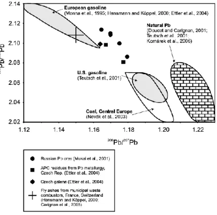
solar system (Komárek et al., 2008). As a consequence, the final Pb isotopic composition depends on the original U/Pb and U/Th elemental ratios, becoming characteristic of a particular geographical location. For this reason, Pb isotope ratios find application in provenance studies in several fields (Sjåstad et al., 2011; Nakata et al., 2015; Dudás et al., 2016; Shepherd et al., 2016; Sjåstad et al., 2016). In environmental science, the use of Pb isotope ratios is a well-known tool, helping scientist to determine the actual presence of Pb pollution and to track the source of anthropogenic inputs. There is a substantial difference between isotopic composition of crustal Pb and that in ores. Pb isotope ratios analysis provides thus an excellent tool to distinguish between local Pb and Pb pollution derived from ores (e.g., anti-knock compounds added to petrol or for industrial use) (Monna et al., 1995; Bollhöfer and Rosman, 2000; Bollhöfer and Rosman, 2001). In environmental samples such as aerosol, sediments and snow, the final isotopic composition is the result of natural and one or more anthropogenic inputs. A way to verify such a possibility is to plot the results in the so called three isotope graph (Figure 7), which is a graphical representation of two different ratios with a common term e.g 208Pb/204Pb vs 206Pb/204Pb.
Figure 7. Example of three-isotope graph showing the isotopic composition of different sources of Pb, based on 206Pb/207Pb vs 208Pb/206Pb (Komárek et al., 2008)
If the results will fall in a mixing line (linear trend) in this diagram, it means that Pb origins from two sources, which are the two end members of the mentioned line. With this representation, the contribution of the 2 sources can be calculated (Komárek et al., 2008). If three end members contribute to the final isotopic composition, the results in the three isotopes graph will plot in a triangular field, delimited by lines connecting the ratios of the three end-members. In such and more complex case, the determination of the single contribution is rather complicated (Vanhaecke and Degryse, 2012). A popular plot in environmental studies is the 207Pb/206Pb versus 208Pb/206Pb, which often shows a linear
trend that can be interpreted as a simple mixture of two Pb sources. Ellam (2010) recently demonstrated that this type of representation could lead to the erroneous conclusion since the linear trend in such representation is inevitable and thus it is not suitable in the case of multiple source mixing. A more reliable test for multiple mixing models can be obtained by plots involving 206Pb/204Pb, 207Pb/204Pb, and 208Pb/204Pb, which highlights the importance of 204Pb isotope. The limitation of this
approach arises from the difficult determination of 204Pb using ICP-MS, as it is the least abundant isotope
(about 1.4% natural abundance) and it is affected by 204Hg isobaric interference.
2. TRACE ELEMENTS MONITORING PROGRAMS
Environmental monitoring describes the processes and activities that are put in place in order to assess the quality of the environment. All monitoring strategies and programs have reasons and justifications which are often designed to establish the current status of an environment or to establish trends in environmental parameters. The ecological, economic and social importance of marine ecosystems being undeniable, a well-planned approach of managing the marine space is essential to achieve sustainability (Jonathan and Gobert, 2016). In parallel with growing concern for environmental conditions, several ocean monitoring programs have been introduced, at national and international levels (Kennish, 1994). Environmental assessment programs have a crucial role in the management of pollution sources and the preservation of marine habitats. The piece of coasts to be managed may be under actual pressure, such as eutrophication and pollution, or it may be under threat of pressure from some proposed development. Historically, most of the water quality investigations have attempted to assess trace elements in aquatic systems by direct analysis of water samples. Many studies have dealt with the determination of total and dissolved TE concentrations through the analysis of filtered and non-filtered water (Cidu and Frau, 2009; Bu et al., 2017). Concentration associated with suspended particulate matters (SPM) is usually indirectly determined as the difference between results obtained by non-filtered water and filtered one. In most of aquatic systems, TE concentrations in SPM are much higher (several order of magnitude) than those in the water samples. Some of the most toxic trace elements (e.g., Hg, As, Cd, Pb and Zn) are strongly associated with sediments and plankton which means that their distribution, mobility and bioavailability in the aquatic ecosystem cannot be solely evaluated by their determination in water (Horowitz, 1991). In Europe, the recent Environmental Quality Standard Directive 2008/105/EC (EQSD, 2008) marked an important step in the use of sediments and biota in environmental monitoring programs, in the frame of Water Framework Directive 2000/60/EC (WFD). Analysis of TE in sediments and biota is widely recognized as an effective approach in water-quality monitoring to provide baseline regional values for local monitoring, for describing the actual contamination levels as well as to identify areas of particular concern (Carere et al., 2012). Most of the toxic substances listed in the principal environmental ranking, accumulate in both sediments and biota.
Is therefore of crucial importance to include sediments, suspended or bed sediments, and biota in a proper environmental monitoring program.
2.1. Trace elements in sediments
Since sediments can act as reservoirs for many trace elements, they are often included in the planning and design of environmental monitoring (Carere et al., 2012; Quevauviller, 2016). One of the great application of sediment analysis in monitoring programs is related to the capability of this final sink to accumulate trace elements and thus providing an historical record of contamination; this property being often observed in sediment cores (Kljaković-Gašpić et al., 2008; Karbassi et al., 2005; Sun et al., 2012; Vallius, 2014). Additionally, under changing environmental and physiochemical conditions (e.g. pH, dissolved oxygen, bacterial actions), TE bound to sediments can be released in the water column, increasing their harmful effect in the environment and food chain (Le Pape et al., 2012; Tripti et al., 2013; Joung and Shiller, 2016).
2.1.1. Sediment components and classification
Marine sediments have very heterogeneous composition, depending on their origin and their geographical localization. The accumulation of TE in sediments depends directly on the nature of sediments. Three main types of sediments can be distinguished based on sources and components (Fütterer et al., 2006): (1) lithogenous (terrigenous or volcanogenic) sediments, transported and dissolved into the oceans as detrital particles; (2) biogenous sediments, formed directly by accumulation of skeletal parts of marine organisms; and (3) hydrogenous sediments, which precipitate directly out of solution as new formations.
Terrigenous material can be transported for several hundreds of kilometers in the form of weathered minerals, by wind. The latter only transport particles of fine grain size, such as silt and clay. Clay minerals constitute up to 50% of entire terrigenous sediments and they are of special importance because of their capability to absorb and release ions (Fütterer et al., 2006). Despite all regional variabilities, the clay mineral composition is rather constant, including only a few basic minerals (Table 2). Regarding the biogenic sediments, they can be considered as all solid hard materials formed in the biosphere. The amount of carbonate deposited in the oceans today is almost entirely derived from biogenic processes. Despite the great variability of marine organisms, only a small group produces hard parts which can contribute to sediment formation in substantial amount. Relevant for sediment formation are only carbonate minerals in the form of aragonite, Mg-calcite and calcite, as well as
biogenic opal in the form of amorphous SiO2·nH2O. Hydrogeneous sediments represent a negligible
contribution to sediment classification, in comparison with previous types. They are mostly formed as direct inorganic precipitates from seawater, like sodium chloride.
Table 2. Mineralogy of main lithogeneous components (adapted from Fütterer et al., 2006)
Principal minerals Idealized composition
Quartz SiO2
Calcite CaCO3
Dolomite (Ca,Mg)CO3
Feldspars KAlSi3O8 – NaAlSi3O8 –CaAl2Si2O8
(repeating units)
Muscovite KAl2[(AlSi3)O10](OH)2
Clay minerals
Kalonite Al2Si2O5(OH)4
Mica group
X2Y4–6Z8O20(OH, F)4
X=K, Na, Ca; Y=Al, Mg, Fe; Z=Si, Al
Chlorite (Mg3-yAl1Fey)Mg3(Si4-xAl)O10(OH)8
Smectite group
e.g. Montmorillonite Na0.33(Al1.67Mg0.33)Si4O10(OH)2•nH2O
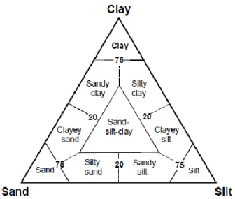
Sediments are also classified according to: (1) the area of their deposition, distinguishing shallow-water deposits, terrigenous deposits in shallow and deep shallow-water close to land and pelagic deposits in deep waters (Fütterer et al., 2006); or (2) the distribution of the grain size. Sediments displays a great variety of grain sizes, from very coarse sand or gravel to very fine-grinded material. The Udden-Wentworth scale pinpoints four major categories, based on the grain size (Udden-Wentworth, 1922): gravel (>2 mm), sand (2 mm-63 µm), silt (63 µm – 3.9 µm), clay (<3.9 µm). Plotting the percentage of these categories in a three-plot diagram results in a graphic classification of terrigenous sediments based on grain size distribution, as shown in Figure 8.
Figure 8. Ternary diagram of sand-silt-clay grain-size distribution showing principal names for terrigeneous sediments (from Fütterer et al., 2006
2.1.2. Factors affecting TE accumulation in sediments
A number of geochemical factors should be considered in the understanding of trace elements behavior in sediments. These factors help in the investigation of TE transport and environmental effects. The identification and quantification of these factors is often called partitioning, and divided into physical and chemical. Physical partitioning involves parameters such as grain size, surface area, magnetic properties etc. while chemical partitioning refers to the determination of chemical components such as carbonates, clay minerals, organic matter, silicates etc. These two types of partitioning are in fact strongly correlated to each other (Horowitz, 1991).
2.1.2.1. Physical factors
The principal physical parameter influencing TE chemistry in sediments is recognized to be the grain size (Thorne and Nickless, 1981; Horowitz and Elrick, 1987). There is a very strong correlation between decreasing grain size and increasing TE concentrations. Fine grained sediments, because of their large surface areas, are the main sites for collection and transport of TE. Nevertheless, TE accumulate on coarse material as well, including sand, but the highest concentrations are usually found in fine particles (Horowitz, 1991). In order to mitigate differences due to grain size, it is possible to perform a normalization with respect to this parameter. A recent study has examined the efficiency of normalization using the <63 µm fraction as normalizing parameter, showing that the possibility to
misinterpretation is quite high. The reason is that this fraction is unlikely to accurately embody the clay content, which represents a major factor in TE adsorption in sediments (Szava-Kovats, 2008). The correlation between grain size and TE content was observed in a broad range of sizes such as <16, <70, <125 µm among others (Beeson, 1984; Horowitz and Elrick, 1987). Additionally different tendency can be observed for different elements, i.e. different slopes when the element concentration is plotted against percentage of fine grain-sized portion of the sediment. The element distribution in different granulometric fractions of the sediment can be very specific and characteristic, thus allowing the differentiation of samples from diverse origins.
The surface area, reported in area per mass, is another very important physical parameter to be considered. It is strongly correlated with grain-size (it increases with decreasing in grain size) but it also depends on chemical composition. This parameters is very important since the majority of processes through which TE are collected, concentrated and retained in sediment fall into the general category of “surface reactions”. It follows that materials with large surface areas are those mainly involved in TE chemistry (Horowitz, 1991). The main process involved in TE collection is the adsorption, which is the condensation of constituents on the surface of another material. Materials with high surface areas can be seen as mechanical substrates upon which the inorganic particles can concentrate without involving chemical reactions. The more the surface area increases the more the capacity of these materials to adsorb TE improves. The surface areas of some substances are shown in Table 3.
Table 3. Surface areas of some materials with diameters <2 µm (data from Forstner and Wittmann, 1981, table from Horowitz, 1991)
Material Surface area (m2/g)
Calcite 12.5 Clay minerals Kaolinite 10-50 Illite 30-80 Montmorillonite 50-150 Iron hydroxide 300 Organic Matter 1900
2.1.2.2. Chemical factors
Several chemical processes govern the chemistry of TE in sediments. Adsorption, precipitation and co-precipitation, organometallic bonding, cation exchange are some of the main chemical processes affecting TE association with sediments or TE release from sediments.
Most of TE behave as cations and are readily sorbed and released on and from surfaces of materials with net negative charge, such as clay minerals, iron and manganese hydroxides and organic matter. This process is called cation exchange and it occurs thanks to the sorptive capacity of different anionic sites such as SiOH, Al(OH)2, AlOH (clay minerals) and -COOH or –OH groups (from organic matter) among
others (Forstner and Wittmann, 1981). The cation exchange capacity (CEC) determines the ability of a material to hold cations, and it has be proven to be correlated with grain size and surface area. Some of the materials with the highest CEC are manganese hydroxide, humic acids and iron hydroxide (Horowitz, 1991). Bearing in mind the strong relation between physical and chemical properties, a number of compounds and substances most important in TE behavior in sediments can be identified. These materials (or geochemical substrates) are characterized by large surface areas, high CEC and they are mostly concentrated in the finer size fractions.
• Fe and Mn oxides are well known for acting as excellent TE scavengers in solutions (Gadde and Laitinen, 1974), they are mostly found in sediments under the form of nodules, micro-nodules and coating. They have been proven to be important concentrators of TE in aquatic systems (Jones and Browser, 1987; Forstner, 1982; Horowitz and Elrick, 1987).
• Organic matters (OM), generally named humic substances (humic acids, fulvic acids, humins) are well known for concentrate TE in soils and sediments (Hirner et al., 1990; Rieuwerts et al., 1998). The capacity of organic matter to concentrate TE varies with the constituent and the type of OM but also to the stability of the TE-organic compound formed. The concentration of aquatic organic matter is indicated measuring the total organic carbon. Negative or no-correlation between OM and some TE were also reported in the literature (Wang and Qin, 2006) showing a very variable interaction which might depends on the source (natural or anthropogenic) of both, OM and TE (Wang, 2008).
• Clay minerals are the main components of fine-grained sediments, characterized by large surface areas per unit mass. They are considered to be the major reasons for enrichment of TE in sediments. The actual role of clays in TE transport and accumulation depends on a number of factors, such as valence of TE, ionic radium, type of mineral (Förstner et al., 1989). It has been proposed that clay minerals might simply provide a mechanical substrate for other materials, such as OM and second minerals, and the latter carry out the actual concentration of TE (Horowitz and Elrick, 1987; Horowitz, 1991).
2.1.3. TE monitoring in sediments
Several trace and major elements have been analyzed in sediment samples in many parts of the world as a mean to provide environmental assessment. Considering that TE natural occur in sediments as primary components of minerals, it is often needed to set a background local level in order to be able to determine whether a high concentration is due to natural or anthropogenic input. It is rather difficult to set a “normal” trace elements concentration, as the natural background play an important role and the concentration ranges can be very wide for the majority of elements, even in pristine areas. For instance concentrations between 1.4-4.9, 673-5075 and 55-389 mg kg-1 for Cd, Cu and Co respectively in
sediments from the Tigris River (Varol, 2011); Vallius et al. (2007) reported values between 7.3-19.1 and 46-83 mg kg-1 for As and Cr respectively in surface sediment from the Finnish coast of the Baltic Sea
while Parra et al. (2015) measured concentrations between 41-1476, 8-17, 6-15, 17-36, 9-20 mg kg-1 for
Cu, Ni, Co, Pb and As respectively in marine sediments from Chile.
The “quantification” of sediment pollution thus needs to be assessed after the evaluation of the extent of TE naturally present in the considered area. For this purpose a chemical normalization is often performed, with respect to reference elements such as Fe and Al (Abrahim and Parker, 2008; Karbassi et al., 2007) but also Mn, Ti and Sc (Zahra et al., 2014; Salati and Moore, 2010) and Li (Aloupi and Angelidis, 2001). The background (BG) concentration can be taken from reported natural abundances in the earth crust or taking as a reference the TE concentration measured in a proved uncontaminated place form the same area of study. Geochemical normalization has extensively been used to calculate enrichment and to reduce heavy metal variability caused by grain size and mineralogy of sediments (Zahra et al., 2014). Using both, background concentrations and normalizing elements, some parameters such as Enrichment Factors, Geoaccumulation Indices, Metal Pollution Indices and Pollution Load indices can be calculated in order to evaluate the extent of metal contamination in the sediments. the results are then evaluated following specific criteria (Guan et al., 2016).
The application of such parameters is nowadays very often used in monitoring studies involving lake, river and marine sediments ad proved to be useful tool in TE pollution assessment. For instance Guan et al. (2016) found rather high Co concentrations in river sediments from the Yellow river (max 339 mg kg -1) but being the BG level around 280 the final enrichment was not considered substantial.
mg kg -1 respectively. As a result the calculated parameters revealed significant anthropogenic influence
for Cu (and other elements) but not for Co.
This approach has also been used for the study of sediment core samples, in order to evaluate a possible TE enrichment during the history, evaluating the vertical variation. In this case the BG value is often taken from the deepest sediment layer collected in the studied area (Veerasingam et al., 2015).
Nevertheless even though a high concentration of TE might not reflect anthropogenic influence it can still represents a threat for other compartments of the environment, adversely affecting for example the aquatic organisms. In order to evaluate such a possibility, sediment quality assessment guidelines are very useful to screen sediment contamination by comparing sediment contaminant concentration with the corresponding quality guideline (Macdonald et al., 1996). Quality guidelines and threshold values for marine sediments (but also for water and some biota) are provided by national and international institution such as EPA (Environmental Protection Agency).
2.2. Trace elements in marine organisms
TE accumulation by living organisms is based on the fundamental characteristics of living cells to take up elements from a solution against a gradient of concentration. This is perhaps most obvious for marine (or generally aquatic) organisms which obtain their nutrients directly from water (mollusks, algae, sponges for instance) (Bowen, 1966). Several studies have been published on the use of different biota and marine organisms to monitor TE in the ecosystem. Aquatic biota represent an incredible source of diversity in their biochemical adaptations to the environment and they are of increasing interest to scientists for several applications (Carpenè et al., 2017). Generally the selected organisms need to have some characteristics, such as being representative of the water body, accumulating one or more priority substances, being sampled on a regular basis without endangering the population of the organism itself. Additionally an adequate amount of sample needs to be available for chemical analysis (AMPS Expert Group, 2005).
2.2.1. Bivalves
Among marine organisms, mollusks such as oysters, mussels, scallops, clams and snails have been often used in monitoring TE contamination in the marine environment. These organisms are known for accumulating toxic elements. Since some of them are consumed as seafood in many countries, they can present a tangible risk for human health (He and Wang, 2013). In terms of human consumption, oysters are often the most important farming species, followed by clams, mussels and scallops. Bivalves have
been also employed as biomonitors of TE pollution in coastal environments because of their widespread distribution (Wang and Lu, 2017). Wide surveys such as the US Mussel Watch Program were put in place, involving the measurement of TE and other contaminants in different species of mussels and oysters and providing a database with results from long term studies (Cantillo, 1998).
Oysters are known to especially accumulate great amounts of Zn and Cu, both essential elements for these organisms. The accumulation varies according to oyster species and elemental availability. Cu and Zn concentrations in oysters collected in relatively clean places were reported to be around 50-100 and 500-2000 µg g-1 respectively (Baudrimont et al., 2005; Wang et al., 2011; Ochoa et al., 2013).
However, very high concentrations of these two elements (>10000 µg g-1) were found in China and
Australia in ecosystems known contaminated by Zn and Cu due to industrial releases (Weng and Wang, 2014 ;Birch et al., 2014). An interesting study recently investigated the Cu and Zn speciation in oysters, finding out that the excess of these elements is “stored” in the organisms tissue in O- and N- complexes, as a way of detoxification (Tan et al., 2015). It has also been reported that Ni, Cr and Pb do not concentrate at such high extent in these organisms, never reaching values reported for Cu and Zn (Wang and Lu, 2017). Pb concentrations reported for oysters are generally lower than 4 µg g-1 , but there were
a few cases where Pb tissue concentrations were high (e.g., up to 58.2 µg g-1 in Persian Gulf, (Heidari et
al., 2013), suggesting a potential Pb contamination in the region. Ni is not often reported but it is generally found in quite low concentration (2-4 µg g-1), except for a study of Weng and Wang, 2014 in
which concentrations up to 43 µg g-1 are reported for oysters from Jiuzhen, China.
Mussels have also been extensively used in TE monitoring studies but again, as for oysters, limited studies have been focused on the comparison of accumulation properties for different species of mussels (Wang and Lu, 2017). Mussels are often used as biomonitors of Cd contamination as they present a response in their accumulation proportional to the external concentration. Nevertheless, Cd is more efficiently removed from mussel’s tissue compared to oyster (Wang and Lu, 2017). Cd concentrations in mussels are usually lower than 2 µg g-1but some high concentrations (>60 µg g-1) were
found in the Gulf of Maine (USA) by Chen et al. (2016). In contrast to oysters, mussels are known to regulate their Cu and Zn tissue concentrations. The values reported for mussels are thus generally lower that those reported for oysters for these two elements. In this regards, bivalves show different accumulation properties and such characteristics have to be taken into considerations when these organisms are used as biomonitors of TE pollution. Among bivalves, clams are generally less studied but
they are considered to have a behavior similar to mussels, with respect to TE accumulation (Wang and Lu, 2017).
Marine organisms have a crucial role in the conversion of TE chemical forms. As already seen in previous paragraphs, the mobility and toxicity of some TE and their bio-availability depends on their chemical forms. The conversion of a given species from a chemical form to another one, can happen as a result of biochemical process, e.g. within the organism’s tissue. For example inorganic mercury is transformed into organic mercury compounds by aquatic micro-organisms and accumulates in the food chain (Hartwig and Jahnke, 2012). The organic mercury compounds, of which methyl-mercury is the most common, are of special concern because of their great toxicity (Coulibaly et al., 2016) since they accumulate in living organisms and damage their central nervous system (Lauwerys et al., 2007). Hg, especially mono methyl-Hg, is also recognized to be biomagnified through the food chain. In this context, it is not surprising that several studies have been focusing on Hg speciation analysis in marine organisms (Leermakers et al., 2005; Spada et al., 2012; Azemard and Vassileva, 2015; Krata et al., 2016; Lang et al., 2017). On the contrary, other elements such as arsenic are transformed in less toxic species by the action of living organisms, as illustrated in paragraph 1.2.1. This is probably the most evident characteristic that differentiates As and Hg, and highlights the important role of biological processes in the aquatic environment.
2.2.2. Sponges
Sponges (Phylum Porifera) are an aquatic filter-feeding group of animals. The group consists of about 15000 species distinguished in three classes (Hooper and van Soest, 2002): the glass sponges (Class Hexactinellida)
• the calcareous sponges (Class Calcarea) • the demosponges (Class Demospongiae)
Adult sponges come in a variety of colors, sizes and shapes including arborescent (tree-like), flabellate (fan-shaped), caliculate (cup shaped), tubular (tube shaped), globular (ball shaped), and amorphous (shapeless) among others. Sponges occupy both freshwater and marine environments, from shallow to abysmal depths, and are common in coral reef, mangroves, and seagrass ecosystems. Some years ago a study proved the ancient origin of sponges, which were shown to be the most primitive metazoans (Clark, 1968). The ancient origin of sponges was also proved by the existence of a poriferan fossil record going back to the Early Vendian (~580 Mya) (Li et al., 1998), and by sponge biomarker
record going back to the Cryogenian period (~750 Mya) (Love et al., 2009). Sponges represent a very important component of the benthic community, and their role in the marine ecosystem is of crucial importance for other organisms such as corals (Wulff, 2001; Diaz and Rutzler, 2001). Sponges have shown to be able to enhance coral survival, to have an important role in carbon and nitrogen cycles in the ocean (Bell, 2008) and to provide habitat for other organisms.
In environmental chemistry, sponges can be used as bioindicators of marine pollution but, studies focusing on sponges are limited in comparison to other marine organisms, such as mussels, oysters, clams. Recently these organisms gained scientists attention as possible biomonitors of TE contamination since they are abundant and widespread, long-living, sessile, and easily sampled and they have shown high tolerance for several pollutants. Additionally sponge communities can remain stable for long time periods, making them suitable model organisms for long and short-term monitoring studies. Sponges are filter feeding organisms, capable to pump very high quantities of seawater (100-1200 mL h-1 g-1).
These filtering capacity are larger than most of other marine organisms (Olesen and Weeks, 1994) such as bivalves (Negri et al., 2006; Gentric et al., 2016). Sponges have also shown a high capacity for TE accumulation in a large time scale (Patel et al., 1985; Padovan et al., 2012) and revealed high tolerance for several pollutants (de Mestre et al., 2012; Batista et al., 2014). They can be considered as ‘‘biological particle traps’’ as they are able to concentrate a wide range of pollutants from both the suspended and dissolved phases, often showing high bio-concentration factors (Berthet et al., 2005; Cebrian et al., 2003). The detection of large quantities of TE in sponges suggests the existence of detoxification systems (Aly et al., 2013). All these characteristics make them suitable as a model organisms for monitoring studies, and their use as TE biomonitors has been proposed in several areas (Negri et al., 2006; Venkateswara Rao et al., 2009; Illuminati et al., 2016). Sponges have also been reported as efficient environmental remediators of different toxic compounds such as the bacterium Escherichia coli (Milanese et al., 2003) and the lindane, an organochlorine pesticide (Aresta et al., 2015). These characteristics, combined with recent interests in sponges as a source of novel pharmaceuticals and bioactive compounds (Anjum et al., 2016; Laport et al., 2009), indicate the possibility for a self-financing remediation program (Gifford et al., 2007).
A common way to evaluate the organisms’ capability to quantitatively accumulate TE is the calculation of bioaccumulation and bioconcentration factors (BAF and BCF). Specifically BAF and BCF are calculated as the ratios between contaminant’s concentrations found in the organism and the corresponding concentration found in water and sediment, respectively (Gobas, 2001).
Most of TE have been shown to be highly accumulated in several sponges species, showing higher BCF >1. The differences in TE accumulation among sponges seem to be strictly dependent on both, the species and the considered element. Among TE, Cu and Zn are usually highly accumulated in sponges because of their essential role: required for sponges growth (Cebrian et al., 2007; Mayzel et al., 2014). The range of their concentrations can be very wide depending on sponge specie and element availability in the environment. For example, Cu and Zn were reported to range between 0.2 and 19 mg kg-1 and 2
and 1397 mg kg-1 respectively in sponges from Southeast Brazil (Batista et al., 2014). Arsenic was also
shown to be highly accumulated in different species of sponges, proving its important role in sponge’s biological processes. High As concentrations were reported in sponges: higher than 100 mg kg-1 by Pan
et al. (2011), but also higher than those usually reported for fishes and other marine organisms such as algae and shellfish (Llorente-Mirandes et al., 2010). Cd was also recognized to be accumulated in sponges: e.g. in all the 16 sponge species analyzed by Mayzel et al. (2014) (BCF up to 60), or in different species of Antarctic sponges analyzed by Negri et al. (2006) and Bargagli et al. (1996). Other elements such as Mo, Ag, Cr and Pb are also often included in studies involving sponges, showing very variable accumulation properties, depending on the species. For example, Gentric et al (2016) reported values up to 12, 1.2, 6.2 and 6.8 mg kg-1 for Cr, Mo, Ni and Pb, consistently higher than a specie of oyster collected
from the same place. Pan et al. (2011) measured TE in different sponges and sediments from Red Sea, showing bioconcentration factors up to 74, 22, 3, 56 and 5 for Cd, Zn, Ag, Cu and As respectively. A particular behavior was observed in the specie Acanthella acuta with regards to Ag, showing very high concentrations in sponge tissue as well as a longer detoxification process (Genta-Jouve et al., 2012).
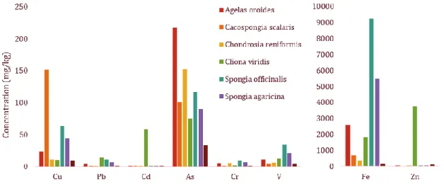
Figure 9. Comparison of TE measured in six sponges species (Cacospongia scalaris, Spongia officinalis, Spongia agaricina,
Agelas oroides, Chondrosia reniformis Nardo and Cliona viridis) and a common mussel (Mytilus galloprovincialis). Adapted from
Perez et al., 2003.
In conclusion, several properties make sponges good models for biomonitor TE pollution in coastal ecosystems. Among TE, Cu and Zn seem to be better accumulated in oysters and mussels. Sponges have shown to be better accumulators of other elements such as As, Ag and Ni.
3. TRACE ELEMENTS ANALYSIS
As a consequence of the increasing interest in TE analyses in different matrices, several techniques have been developed in the last decades. The main challenges are linked to the need for precise and accurate determination of these low-level analytes occurring usually in complex matrices with particular chemical and physical features. Accurate TE determination in environmental samples is of primary interest, as national, European and international legislations have reduced the maximum concentration of several analytes in different environmental samples. A variety of techniques based on different principles can be applied : electroanalytical methods, atomic spectrometry, X-ray and nuclear techniques (Brown and Milton, 2005).
Atomic spectrometry techniques, such as Atomic Absorption Spectrometry (AAS), Inductively Coupled Plasma Atomic Emission Spectrometry (ICP-AES) and Inductively Coupled Plasma Mass Spectrometry (ICP-MS) are very sensitive and capable of determining several elements within a limited amount of sample in a few minutes. These methodologies are extremely useful for the determination of
total amount of TE in environmental samples (Bermejo-Barrera et al., 1996; Damiano et al., 2011; Barats et al., 2014; Wysocka and Vassileva, 2016; Wang et al., 2017). The atomic spectrometric techniques used in this study (AAS and ICP-MS) imply the atomization and ionization of the samples, and their analysis according to their interaction with electromagnetic radiation or their mass (Brown and Milton, 2005). Very often the analysis of environmental samples by AAS and ICP-MS implies a sample preparation step: e.g., microwave digestion and solid-liquid extraction. This step might be responsible for systematic bias due to analyte loss, contamination, variability in analyte recovery. This preparation can represent a significant contribution to the total uncertainty (Barwick and Ellison, 1999). The increasing need for reliable data on TE concentration in a variety of environmental matrices has led to the production of several Certified Reference Materials (CRMs) used to assess the quality of the analytical method both in the development and in the application stages. The use of CRMs, when available, is especially needed when sample preparation is needed, to verify the correctness of the procedure and to identify the source of possible errors related to recovery and contaminations. The use of procedural blanks is also of crucial importance for the assessment of the method quality and to check possible contaminations occurring during the sample preparation.
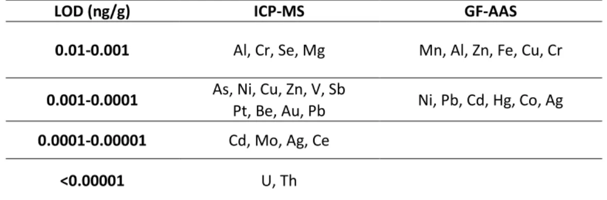
Graphite furnace (GF) AAS is often directly compared with ICP-MS in the literature (Ndung’u et al., 2003). Table 4 shows a comparison between typical Limits of Detection (LOD) of these techniques. ICP-MS is a more sensitive analytical technique, with the great advantage to be multi elemental, while AAS is a mono-elemental technique.
Table 4. Comparison of approximate LOD between ICP-MS and GF-AAS (Adapted from Brown and Milton, 2005)
LOD (ng/g) ICP-MS GF-AAS
0.01-0.001 Al, Cr, Se, Mg Mn, Al, Zn, Fe, Cu, Cr
0.001-0.0001 As, Ni, Cu, Zn, V, Sb Ni, Pb, Cd, Hg, Co, Ag Pt, Be, Au, Pb
0.0001-0.00001 Cd, Mo, Ag, Ce
<0.00001 U, Th
3.1. Atomic Absorption Spectrometry
AAS is particularly indicated for the measurement of major elements. It can be used with Flame (F-AAS) or Graphite Furnace (GF-AAS or ET-AAS) atomizers. F-AAS typically works with liquid, and it is relatively inexpensive and simple to operate. It requires a large sample volume (around 10 mL). This analytical method is not indicated for some refractory elements such as Zr, As and Se, since the flame working temperature are not sufficiently high, but it is particularly indicated for the measurement of major elements in sediment and soil samples previously mineralised, e.g. in sediments such as Fe, Zn and Mn (10-10000 mg Kg-1) (Loring and Rantala, 1992). GF-AAS exibits LOD typically 10-100 times lower
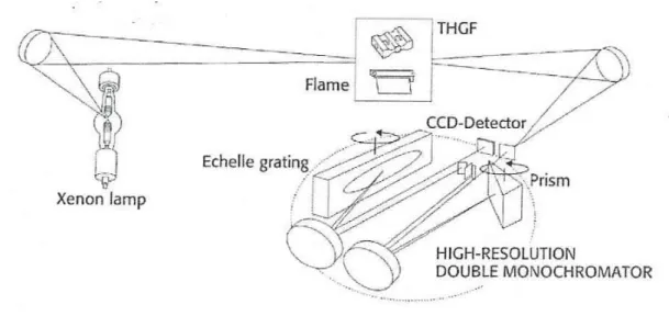
compared to F-AAS (Brown and Milton, 2005). The atomization takes place in a graphite furnace at higher temperature than atomization in the flame and the samples can be liquid or solid. Solid Sampling (SS) GF-AAS is very promising and finds already several application (Belarra et al., 2002). Since the sample preparation step is not necessary, the risk of contamination and losses of analyte are removed. Relatively small quantities of solid (50-500 mg) may be analysed. Many of the interferences from which GF-AAS used to suffer (mostly associated with the sample matrix) can now be overcome with a combination of background correction and matrix modification (Brown and Milton, 2005). Another advantage of the use of (SS) GF-AAS is the possibility to work with fast programs, in which drying and pyrolisis steps are drastically shortened or even eliminated (Mandjukov et al., 2015). This aspect not only represents an advantage since it reduces the analysis time, but it also reduces the possibility of analyte losses, especially for volatile elements such as Hg and As. The recent introduction in the market of instruments equipped with High Resolution Continuos Source (HR-CS) and a charged coupled device (CCD) array detector has allowed several limitation due to classical line sources (LS) to be overcome (Figure 8). The continuous background covering the spectral range observed by the array detector is corrected automatically using correction pixels on both sides of the analytical line. In difference, the structured background can be corrected using reference spectra and a least-squares algorithm (Welz et al., 2007). In such configuration, it is possible to monitor not only the absorbance over time, as in classic LS AAS but a 3D information is also provided, about absorbance over time and over wavelength. This helps in avoiding interferences and generally in the method development stage.
Figure 10. Representation of optical system in HR-CS-AAS (Analytic Jena, ContrAA 600)
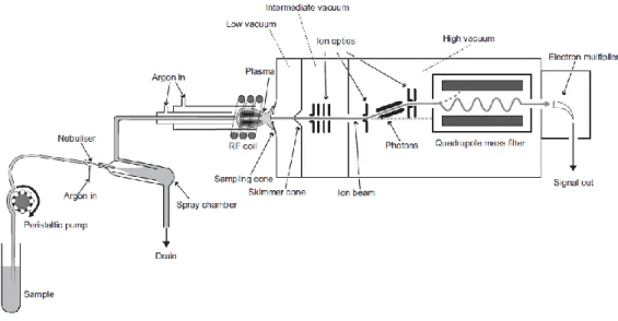
3.2. Inductively Coupled Plasma Mass Spectrometry
Since its introduction in the market more than 30 years ago, ICP-MS has been gaining popularity among the techniques for TE determination for several reasons. First of all, in comparison with AAS, it can detect multiple elements in a few minutes single run. Additionally, its detection limits are close to or below the ng L-1 or the part per trillion (ppt) for most of the elements in the periodic table. Furthermore,
ICP-MS gives the opportunity to perform isotopic analysis, opening to a larger application field in comparison to other techniques. Most of the elements in the periodic table are measurable by ICP-MS, with some exceptions (e.g. F, H, He, Ar). There are some different configuration commercially available which can differ in the design of specific parts such as the introduction system (nebulizer and spray chamber), the interface and the mass analyzer. The working principle of this technique includes the introduction of a liquid sample, usually through a peristaltic pump, into a nebulizer where it is converted in fine aerosols with an argon gas (Thomas, 2003). The fine aerosol is separated from the rest of the sample and carried through an injector to the plasma thanks to an Ar flux of 1 L min-1. The Ar plasma is
formed inside a quartz torch by the interaction of an intense magnetic field (produced by a radio frequency generator) on a tangential flow of Ar gas. In this condition, the Ar is ionized and when a spark act as a source of electrons, a very high-temperature (about 10000K) plasma discharge is formed. The plasma is responsible for atomization and further ionization of the analytes of interest. The energy available in an Ar plasma is about 15.8 eV which is sufficient to ionize most of the elements in the periodic table (Thomas, 2003).