HAL Id: hal-01995328
https://hal.archives-ouvertes.fr/hal-01995328
Submitted on 11 Feb 2019
HAL is a multi-disciplinary open access archive for the deposit and dissemination of sci-entific research documents, whether they are pub-lished or not. The documents may come from teaching and research institutions in France or abroad, or from public or private research centers.
L’archive ouverte pluridisciplinaire HAL, est destinée au dépôt et à la diffusion de documents scientifiques de niveau recherche, publiés ou non, émanant des établissements d’enseignement et de recherche français ou étrangers, des laboratoires publics ou privés.
To cite this version:
Bruno Bachelet, Philippe Mahey, Rogério Rodrigues, Luiz Fernando Soares. Elastic Time Computa-tion for Hypermedia Documents. VI Brazilian Symposium on Multimedia and Hypermedia Systems (SBMìdia), Jun 2000, Natal, Brazil. pp.47-62. �hal-01995328�
Elastic Time Computation for Hypermedia Documents
Bruno Bachelet* Philippe Mahey* Rogério Rodrigues+ Luiz Fernando Soares+
*{bachelet, mahey}@isima.fr
LIMOS, CNRS ISIMA, Université Blaise Pascal
+{rogerio, lfgs}@inf.puc-rio.br
Departamento de Informática PUC-Rio
Abstract
This paper presents a new elastic time algorithm for adjusting hypermedia document presentation in order to avoid temporal inconsistencies. The algorithm explores the flexibility offered by some hypermedia models in the definition of media object duration and uses this flexibility for choosing the objects to be stretched or shrunk in such a way that the best possible quality of presentation is obtained. Our proposal is based on the “out-of-kilter” method for minimum-cost flow problems and it seems to offer more flexibility to model real-life applications in comparison with other previous proposals based on the simplex method.
1. Introduction
This paper focuses on the coupling issues between the specification and presentation phases of a hypermedia system. More precisely, it aims at defining tools for elastic time computation. Elastic time computation, as formerly named by [KiSo95], tries to adjust document presentation in order to guarantee its temporal consistency. The goal is accomplished by stretching and shrinking the ideal duration of media objects. Of course, elastic time computation is only meaningful when hypermedia systems are based on document models that provide flexibility in the definition of media object presentation characteristics. Usually, the duration flexibility specification contains some kind of cost information that gives the formatter, that is, the machine responsible for controlling the document presentation, a metric for maximizing the global quality of the presentation, while obeying other criterion, such as trying to minimize the number of objects that will be stretched or shrunk. Besides the difficulty of modeling such problem in real-life situations, where a user interaction induces non deterministic data or where the definition of the quality measure depends on multi-criterion analysis, we must also keep in mind that the algorithms should run in very short execution time.
Some proposals for elastic time computation have been addressed in the literature [BuZe93a, KiSo95, SaLR99]. However, Firefly [BuZe93a] and Isis [KiSo95] have limited their study to simplified academic models which lead to small-scale linear programs solved by the simplex method. Furthermore, the algorithms are suitable only for compile time, that is, before the beginning of the document presentation. Madeus formatter [SaLR99] presents a solution for runtime adjust (adjustments during presentation), but it is based on a greedy approach, ignoring any cost specification to improve the document quality. In this paper, we propose a new algorithm based on the “out-of-kilter” method for minimum-cost flow problems [Fulk61], which allows much more flexibility to model real-life applications. The algorithm is validated in the deterministic case with general convex cost functions, being suitable for both compile time and runtime.
The paper is organized as follows. Sections 2 and 3 present the general ideas about specification and formatting of a complex hypermedia document. Then, in Section 4, we present the temporal graph and the minimum-cost tension problem which underlies the decision model. We describe and justify the use of the out-of-kilter algorithm, focusing on the possibility of distributing the computation among the document objects. Indeed, each arc of the temporal graph is individually forced to optimality, which induces a high degree of flexibility to recover a sub-optimal solution when some unpredictable event affects the precompiled presentation.
2. Temporal specification in hypermedia documents
The presentation specification of a hypermedia document is accomplished by the definition of its basic elements (text, audio, video, etc.) and their spatial and temporal relationships. The basic elements, usually called media objects or content nodes, have as main attributes the content to be presented (often a reference to the content) and some additional parameters that define the object presentation behavior (e.g., duration, spatial characteristics, anchors, etc.). Relationships among media objects are usually specified by links, compositions, or both, depending on the conceptual model in use. Examples of the use of compositions can be found in the parallel and sequential elements of SMIL [W3C98], in Isis primitives [KiSo95] and in the parallel and sequential contexts of NCM [Soar00]. Examples of the use of links can be found in HTML hyperlinks, NCM spatio-temporal links [Soar00, SoRM00], in timed Petri net transitions of OCPN [LiGh90] and TSPN [DiSé94], and in Firefly temporal point nets [BuZe93a].
In spite of how they are specified, temporal relations can be classified into: causal relations and constraint relations. Causal relations, also known as event-based relations, are based on conditions and actions. They define actions that must be fired when some conditions are satisfied. An example of causal relation is: “when video A presentation finishes, stop playing audio B”. Constraint relations specify restrictions that must be satisfied during a presentation, without any causality. An example of constraint relation is: “video A and audio B must finish their presentations at the same time”. Although similar, the former example (causal relation) does not ensure that both media objects will be entirely played. If A finishes its presentation first, B presentation will be interrupted. On the other hand, the latter example (constraint relation) specifies that the presentations should finish at the same time and in a way that both media objects have all their content presented. It is worth mentioning that this constraint must be satisfied if and only if both media objects are presented simultaneously (only the presentation of A or only the presentation of B also satisfies the constraint relation).
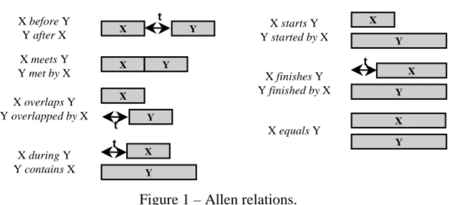
Both kinds of relations are important to hypermedia presentation modeling. Models based only on temporal constraints do not capture the causality intrinsic to hypermedia scenarios and can lead to specification ambiguities. For instance, let us take the meet constraint relation of Allen [Alle83], exemplified in Figure 1. Just specifying that a media object X meets another media object Y does not let one know if the end of X causes the start of Y, if the start of Y causes the end of X, or if the end of X should coincide with the start of Y, without any causal relationship. On the other side, models purely based on causal relations do not allow an author to specify, for example, that two media objects should finish their presentation simultaneously, both having their content entirely presented, as previously exemplified.
t X Y X Y X before Y Y after X X meets Y Y met by X t X Y X overlaps Y Y overlapped by X t X Y X during Y Y contains X X Y X starts Y Y started by X X finishes Y Y finished by X X Y t X equals Y X Y
Figure 1 – Allen relations.
Models based only on causal relations cannot generate temporal inconsistencies. However, they can lead to spatial inconsistent specifications, for example, resource contention. In these models, it is also possible to have actions ignored during the presentation (e.g., to finish a media object that is no more being presented), as well as unreachable actions (those whose conditions will never be satisfied)1. On the other side, models with constraint relations can have temporal inconsistencies. For these models, it is important to verify whether all constraints can be satisfied. From now on, this paper always assumes hypermedia models with both causal and constraint relations.
Regarding temporal consistency checking, it is desirable to have models that allow the specification of a flexible duration for media object presentation, taking advantage of the fact that several media can be temporally stretched or shrunk, without impairing human comprehension. Instead of taking an inflexible ideal duration specification that can lead to inconsistencies, now it is possible to present a consistent document, even with some loss of presentation quality. However, with the introduction of flexibility, besides verifying the temporal consistency of a document, it will be necessary to find the best media object duration value that satisfies all given temporal constraints and leads to the best possible presentation quality of the whole document. Obviously, temporal inconsistent documents may still exist, since the range of adjustments is usually limited.
The basic unit for specifying relationships among media objects defines the hypermedia model granularity. We follow the definitions used in Pérez-Luque and Little’s Temporal Reference Framework [PéLi96] and call the basic unit for defining relationships an event. An event is an occurrence in time that can be instantaneous or can occur over some time period. We classify events into three types. A presentation event is defined by the presentation of a media object as a whole or some part of its content. Analogously, a selection event is defined by the selection of part or the entire content of a media object. Finally, an attribution event is defined by the changing of an attribute value of a media object. Note that the start or end of a presentation event is also an event, in this case, an instantaneous event.
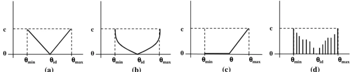
Models that support presentation flexibility should define duration as cost functions. The idea is to allow an author to specify a function “duration versus cost”, where minimum, ideal and maximum values are defined for the duration of each presentation event that constitutes the object presentation. Figure 2 shows examples of cost functions. Intuitively, these functions give the cost for shrinking or stretching the duration from an ideal value, where the ideal value
is given by the function minimum point2. It is also important to allow duration to be specified not only by real values, but also by unpredictable values. Media objects that are presented until some external action interrupt them and media objects that finish their presentations by themselves but in some instant not known a priori are examples of events with unpredictable duration. θθθθmin θθθθmax 0 c θθθθid θθθθmin θθθθmax 0 c θθθθ θθθθmin θθθθmax 0 c θθθθid 0 c θθθθmin θθθθid θθθθmax (a) (b) (c) (d)
Figure 2 – Examples of cost functions. a) Continuous linear function with one ideal value (θid). b) Continuous non-linear function with one ideal value (θid). c) Continuous linear function with multiple ideal values ([θmin,θ]).
d) Discrete function with one ideal value (θid).
Based on cost minimization, it is important to implement algorithms that compute, for each event, the expected duration that offers the best presentation quality for the whole document. This computation mechanism is called elastic time computation in [KiSo95] and is the focus of this paper. The next section comments issues related to hypermedia formatters, emphasizing when the elastic time computation should be done. Before, however, we must define some concepts that will be necessary:
i) An event E1 is said to be predictable in relation to another event E2 when it is possible to
know, a priori, E1 expected start time in relation to E2 occurrence. Note that a constraint
relationship between two events does not make them predictable in relation to each other. ii)We define a relatively predictable temporal scenario (RPTS) as a sequence of related event
occurrences in time. An event E pertains to an RTPS if it is predictable in relation to at least one event of the same RTPS, or if there is at least one event in this RTPS that is predictable in relation to E.
3. Hypermedia formatter
The formatter is responsible for controlling the document presentation based on its specification and on the platform (or environment) description. Usually, the formatter builds an execution plan (a schedule) to orchestrate the presentation. We can divide the formatter into two main phases [BuZe93b], concerning the moments where schedule calculation and consistency check can be done: before the document presentation and during the document presentation. Considering the first phase, we can further divide it into two other phases: during and after the authoring process. Hence, we split the formatter into three main elements. The
pre-compiler performs formatting tasks during authoring phase. The compiler is responsible
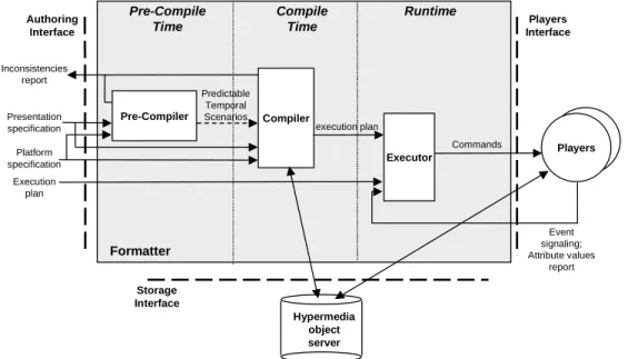
for building the execution plan from an entire document specification and a platform description, before the beginning of its presentation. The executor controls the document presentation and updates the execution plan at runtime. Figure 3 illustrates the hypermedia formatter architecture formed by these three main elements and places the formatter in a hypermedia system environment.
As mentioned, the pre-compiler is indeed a support to the authoring environment. Its main function is to check the temporal and spatial consistency of each RPTS of a document. The pre-compilation is an incremental compilation done during authoring time. It can help the author finding errors, giving an instantaneous feedback whenever any inconsistency is detected, like mismatched time relationships (temporal inconsistency), or conflicts in a device use (spatial inconsistency) in an abstract and ideal platform. Pre-compiler computation can also be stored in order to decrease the time spent by the compiler elastic time calculation.
Pre-Compiler Compiler Executor Event signaling; Attribute values report Execution plan Players Interface Commands execution plan Presentation specification Formatter Runtime Compile Time Pre-Compile Time Hypermedia object server Storage Interface Platform specification Authoring Interface Inconsistencies report Predictable Temporal Scenarios Players
Figure 3 - Hypermedia formatter architecture.
The compiler is responsible for building the execution plan from a complete document presentation specification and a platform description. The compiler should obtain all existent
RPTSs and compute, for each event in each RPTS, the expected duration that leads to a
maximum quality of presentation warranting the document temporal and spatial consistency. Based on the first media object (presentation event) to be presented, the compiler obtains the
RPTS that contains this event and transforms it in the document absolutely predictable temporal scenario (APTS). This procedure is similar to the Firefly formatter proposal
[BuZe93a].
Another important task that should be done by the compiler is to evaluate, from the platform specification, the preparing duration of each presentation event. The idea is to estimate the time to pre-fetch the media object content in order to minimize the delay between the start action and the effective start of the presentation of a media object content. We will not consider pre-fetch computation and heuristics in this paper.
The executor main functions consist in instantiating players to present media objects, interacting with the instantiated players to be notified when event state changes (e.g., start to be presented, finish to be presented, start to be selected, finish to be selected, etc.) and issuing messages to the instantiated players when actions must be executed (e.g., pause, resume, change rate, etc.). When any event state change notification is sent by a player, the executor checks if the signalized occurrence starts a new RPTS. If so, the executor merges the RPTS with the APTS. In any case, the expected times in the execution plan are checked to see if some adjustment is needed. Adjustments may be done through messages sent to controllers,
telling them, for example, to increase or decrease the presentation rate.
Our final goal is to define a method for elastic time computation for pre-compile, compile and execution time. We are interested not only in minimizing the cost of shrinking and stretching, but also in:
1. Minimizing the number of objects that will have events with expected duration different from ideal duration (if there is more than one optimal choice).
2. Choosing the fairest solution that spreads changes in the ideal duration across the objects, in the case that there is more than one solution that satisfy the previous goal.
3. Minimizing the total cost of shrinking and stretching, given a fixed duration for the whole document presentation.
4. Finding the shortest and longest possible duration for the document.
5. Evaluating new ranges for which the temporal consistency of the document is valid, when a media object begins to be presented. This will be very important to help the executor in adjusting object duration on-the-fly.
During runtime, mismatches3 are detected only when portion of the document has already been presented. This delay in detection limits the ability of the executor to smooth out mismatches. During compile time the possible mismatches can be smoothed out improving the appearance of the resulting document. However, only at runtime, unpredictable behavior can be handled. These are the reasons why we need a formatter supporting both compile time and runtime adjustments. Another important issue is that when runtime mismatches cause adjustments in event duration, the expected duration of the subsequent events should be recomputed, since the calculus made at compile time is no more valid. The formatter should run again the elastic time algorithm, now considering the exact duration of the already presented events and the real-time computation requirement. Thus, we also have as a goal: 6. Finding an algorithm that can take profit of the results computed before happening the
mismatch, in order to improve the calculus performance that must be done on-the-fly. The real time calculus may require heuristics, since the optimum calculus can be very expensive. The study of heuristics for elastic time computation at runtime was left as a future work.
This paper is the first step towards our final goals. Here some simplifications are made, as explained in the next section.
4. Elastic time computation
This section presents a graph-theoretical model and a specific algorithm to compute the event optimal duration with respect to some quality criterion and considering some simplifying hypotheses. Our computational approach aims at increasing progressively the sharpness of the model to cope with more realistic situations as described as our final goals at the end of Section 3. We first define the temporal graph, which is used to model the predictable temporal
3 We say that a mismatch occurs when the expected time for an event occurrence, defined by the formatter, is no
scenarios defined in Section 2. Our model was inspired by the early work of Buchanan and Zellweger [BuZe93a]. We suppose that all events are predictable so that the model is completely deterministic4. Algorithmic issues are then discussed to solve the optimization problem as a minimum-cost tension problem in a directed graph with convex arc-separable cost functions. We propose here an adaptation of the ‘out-of-kilter’ method to solve real instances in reasonable time.
4.1 The temporal graph
The basic model is a directed graph G=(X,U), where X is the set of nodes and U the set of arcs (let n= X and m=U ). Nodes represent instantaneous events (the start or end of a presentation event), and arcs represent the precedence relations between these events. Head and tail nodes are added to connect all nodes with no predecessor or successor, respectively, in order to represent the start and the end times of the temporal scenario. Except for the head outgoing arcs, each arc is assigned a cost function. The function defines a feasibility interval
[
min max]
, uu θ
θ , containing an ideal length
θ
ˆu and is supposed to be convex on the feasibility interval.When two or more arcs are incident to a common node, synchronization constraints occur which correspond in terms of graph theory to the existence of cycles made of two directed paths. A graph which represents these synchronization constraints will be called a temporal
graph.
4.1.1 From the author’s specification to the graph representation
We must first observe that, with the temporal graph, we do not intend to model the whole author’s specification. Only the main part of the temporal constraints will be represented. Here are some examples of how to model author’s specification by the temporal graph:
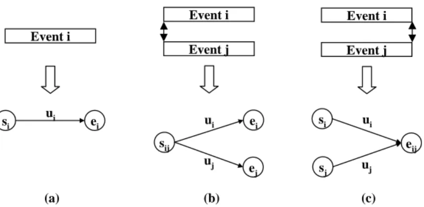
• Let i be a presentation event, as defined in Section 2 and presented in Figure 4a. In the temporal graph, i is modeled by two nodes, si and ei, that represent the start (si) and end
(ei) of the event i occurrence. Note that some actions, like the preparation (pre-fetch) of the
event, are not considered here. An arc ui is also created to model the duration of event i.
The cost function related to this duration is then assigned to ui.
• Consider now two presentation events, i and j, that must start at the same time, as shown in Figure 4b. In the temporal graph, i and j are modeled as above, but the nodes si and sj
are merged to be a single node sij.
• Similarly, if i and j are two presentation events that must end at the same time, as illustrated in Figure 4c, the nodes ei and ej are merged to be a single node eij.
Note that the resulting graph can be a multigraph. Indeed, two events specified with the same starting and ending time will be represented by two arcs with the same source and target nodes.
4
The algorithm we present should be applied in each predictable temporal scenario independently. We left as a future work the problem of handling unpredictable events and efficient merging the relatively predictable temporal scenarios with the absolutely predictable temporal scenario.
Event i si ui ei Event i sij ei ui Event j ej uj Event i si eij ui Event j uj sj (a) (b) (c)
Figure 4 –Temporal graph representation for authors’ specification.
We will now recall some definitions which are useful for the description of the mathematical model (all related notions can be found in [AhMO91]). Given a graph:
i. A cycle is a chain of arcs with a start node coinciding with the end node and an arbitrary direction. For instance, an elementary cycle is the one formed by two paths with the same source and target nodes.
ii. A cocycle is associated with a cutset of the graph that partitions the nodes into two disjoint subsets. The cocycle is the set of arcs that connects one subset of nodes to its complement.
iii. A flow is a vector of values assigned to each arc, such that the flow conservation law is satisfied at each node (thus, the algebraic sum of the flow values on a cocycle is necessarily zero).
iv. Potential is a value assigned to a node.
v. A tension is a vector of values assigned to each arc, such that each tension value of an arc is the difference between the potential of its end nodes (thus, the algebraic sum of the tension values on a cycle must be necessarily zero).
Back to the temporal graph, if an initial date
π
0is arbitrarily assigned to the head node, we can assign a dateπ
i to each node i, which we call the potential of the node. The duration of an object associated to a given arc u=(i,j) can be seen to be the difference of the potentials of its end points. This is indeed the definition of a tension vector on the graph, i.e. such thati j
u
π
π
θ
= − on each arc u. The problem is then a minimum-cost tension problem on the temporal graph [BeGh62]. Using vectorial notation and the incidence matrix of the graph, i.e. the(
m×n)
matrix A with elements aiu equal to -1 (if u goes out of node i), +1 (if u goes intonode i) and 0 (for all other rows), the problem is simply:
Minimize ( u)
ucu
θ
∑
Subject to
θ
= ATπ
,θ
min ≤θ
≤θ
maxNote that the problem can be modeled without introducing potential variables, but we need to know a priori all the synchronization cycles. If S is the arc-cycle matrix where each column is the incidence cycle vector, then θ =ATπ ⇔STθ =0. We can thus introduce flow vectors on the temporal graph which are indeed orthogonal to the tension vectors, i.e. which are linear combinations of the cycle vectors: ϕ =Sδ . The interpretation of these flows comes out of the
general optimality conditions for the minimum-cost tension problem:
( )
u u uc' θ =ϕ on each arc, such that θumin <θu <θumax
( )
0'u u − u ≥
c θ ϕ on each arc, such that θu =θumin
( )
0'u u − u ≤
c θ ϕ on each arc, such that θu =θumax
Thus, the flow value is the marginal cost of the decision on the arc (positive for stretching, negative for shrinking and zero for keeping the object duration with its ideal value). The above conditions are often called the kilter conditions for arc u [Fulk61]. An immediate consequence is that, if two arcs belong to the same paths in the same cycles, i.e. if they belong to a common sequence of presentation with no synchronization constraint between them, they have the same marginal cost.
4.2 Feasibility issues
In the deterministic case, a feasible schedule is characterized by the following conditions. For each synchronization cycle consisting of two paths p and p’, we have:
≤ ≤
∑
∑
∑
∑
∈ ∈ ∈ ∈ p u u p u u p u u p u u max ' min ' max minθ
θ
θ
θ
Consequently, the flexibility interval for a given cycle (p,p’) is
{
} {
}
[
max]
' max min ' min , min , ,max
θ
pθ
pθ
pθ
p , where θpstands for the total path duration. The aboveconditions guarantee that these intervals are non empty.
Finding out an initial feasible tension is by itself an interesting issue. It should be used at real-time presentation when some unspecified event affects the predefined schedule. A very simple and efficient algorithm can be used to solve that problem. It starts with a null tension and, for each arc u, where θu ≤ au, a cocycle containing u can be found, for which the tension can be
increased without making any other arc incompatible. The maximum increasing value is determined and applied to this cocycle. If θu is still inferior to au, another cocycle is searched
to increase the tension of u, else it goes on with another incompatible arc.
4.3 An out-of-kilter algorithm to solve the tension problem
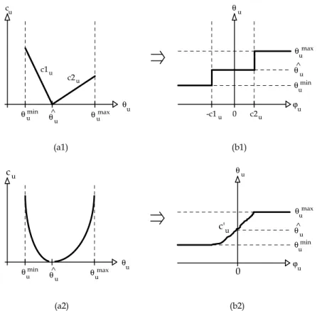
We will now present an adaptation of the out-of-kilter method [Fulk61], first applied to minimum cost tension problems by Pla [Pla71] in the linear case. Polynomial and strongly polynomial algorithms have been recently studied [Hadj96], but their performance in the convex case are still too slow for our purpose. The out-of-kilter algorithm is a primal-dual method which updates tensions and flows, iteratively, until optimality is reached. The main advantage is that the computations are distributed among the arcs, allowing much more flexibility than direct methods. The key tool is the kilter curve which represents the local optimality condition on a specific arc. We consider here two kinds of costs: piecewise linear costs (Figure 5a1) and convex smooth costs (Figure 5a2).
(a1) (b1) ^ θ c ϕ θ 0 u u u u c2u -c1u c1u c2u θ θmin max θumax θumin u u θu ^ θu c 0 u c'u (a2) (b2) u u ϕu θ u max θumin θu θ θmin θ^ max θu u ^ θu
Figure 5 – a*) Cost functions. b*) Kilter curves. *1) Piecewise linear. *2) Convex smooth.
Consider now the kilter curve of an arc u relating its tension θu with its flow ϕu. For the linear
cost, it is represented by Figure 5b1 and for the convex cost, it is shown by Figure 5b2. In both cases, it is said that an arc u is in-kilter if the pair (θu ; ϕu) lies on the curve, else the arc is said
out-of-kilter. We can easily prove that if all the arcs of the graph are in-kilter, then the tension is minimum (see the optimality conditions in Section 4.1). So, all the difficulty is to bring all arcs on the kilter curve. We first explain how to perform that for piecewise linear costs. Then, we detail it for the convex costs. This solution strategy is inspired in [Pla71] and [Hadj96] to solve the minimum cost tension problem with linear costs.
4.3.1 Piecewise-linear costs
First, we classify the arcs of the graph into 4 categories: 1. the arcs that are below the kilter curve,
2. the arcs that are above the kilter curve,
3. the arcs that are on a horizontal part of the kilter curve, 4. the arcs that are on a vertical part of the kilter curve.
For the arcs of category 1, their tension must be increased or their flow must be decreased in order to improve their position towards the kilter curve. For the arcs of category 2, their tension must be decreased or their flow must be increased. In categories 3 and 4, the arcs are in-kilter. For the arcs of category 3, only their flow can be modified without making them out-of-kilter. For the category 4, only their tension can be modified.
Following the seminal work of Fulkerson [Fulk61], we can set that:
• for an arc u of category 1, we can find either a cycle containing u for which the flow can be decreased, or a cocycle containing u for which the tension can be increased;
• for an arc u of category 2, we can find either a cycle containing u for which the flow can be increased, or a cocycle containing u for which the tension can be decreased.
These statements allow us to present the following algorithm that improves the position of an arc to its kilter curve:
algorithm improveArc: if (u is black) then
find a cycle γ to decrease the flow of u or a cocycle ϖ to increase the tension of u;
if (cycle found) then
find λ the maximum value the flow on γ can be decreased; ϕ = ϕ – λγ;
else (cocycle found)
find µ the maximum value the tension on ϖ can be increased; θ = θ + µϖ;
end if;
else /* u is blue */
find a cycle γ to increase the flow of u or a cocycle ϖ to decrease the tension of u; if (cycle found) then
find λ the maximum value the flow on γ can be increased; ϕ = ϕ + λγ;
else (cocycle found)
find µ the maximum value the tension on ϖ can be decreased; θ = θ - µϖ;
end if; end if;
Then we propose the following method to make all the arcs in-kilter, what determines the minimum cost tension. It just applies the previous algorithm successively and repeatedly upon each arc of the graph until all the arcs are in-kilter:
algorithm linearInKilter: make θ compatible;
ϕ = 0;
while (an arc u is out-of-kilter) do for all arc u do
if (u out-of-kilter) then improveArc(u); end for;
end while;
4.3.2 Convex Costs
The method is a bit different for the case of general convex costs. Indeed, we previously saw that, to improve an arc, either the tension or the flow of other arcs are modified, but never both of them at the same time, because it is very difficult to manage this case. However, we sometimes need to move an already in-kilter arc along the kilter curve. As the kilter curve is no more made of horizontal and vertical lines, we should modify at the same time the tension and the flow of such arcs. To avoid that, we approximate the kilter curve by a staircase curve. We use the method presented for the linear costs to bring all the arcs on their approximate
kilter curve and then we improve the approximation of the curve. The procedure is repeated until we obtain the desired precision. It is recommended to start with a weak approximation and then progressively improve it instead of directly starting with a sharp approximation. We outline below the algorithm for this method where p is the precision:
algorithm convexInKilter:
ε = 0.1 x sup {bu – au, u in U};
while (ε > p) do
make all the arcs in-kilter with the ε precision; /* Uses the linearInKilter algorithm. */
ε = sup{0.1ε,p}; end while;
5. Computational results
We present now computational results obtained by the out-of-kilter algorithm. First, we analyze the results for the case of piecewise costs and then for the case of convex costs. In both cases, solution times are expressed in seconds. They came from tests on a RISC 6000 166 MHz biprocessor under an AIX Unix operating system. We used the C++ language and its object-oriented facilities to code the algorithms. For the different methods, we consider the operation of finding a cycle or a cocycle as a single operation. For the CPLEX software, an iteration is one iteration of the SIMPLEX method. Finally, all the results (time and number of iterations) are averaged on series of 10 tests upon randomly generated problems. We then compare these results with results on more organized graphs called series-parallel graphs.
Number of Nodes Number of Arcs CPLEX Iterations CPLEX Time In-Kilter Iterations In-Kilter Time 50 100 62 0.3 150 0.2 50 200 135 0.6 271 0.5 50 300 198 0.9 374 0.8 50 400 254 1.3 482 1.2 50 500 277 1.6 595 1.6 100 200 143 0.6 286 0.7 100 400 323 1.4 532 1.9 100 600 424 2.3 749 3.2 100 800 512 3.1 958 4.3 100 1000 603 4 1166 5.6 500 1000 1152 7.6 1365 15 500 2000 2129 22 2609 45 500 3000 3034 42 3760 77 500 4000 3387 57 4831 114 500 5000 3687 72 5930 152 1000 2000 2642 30 2601 58 1000 4000 5012 118 5125 171 1000 6000 6143 195 7433 309 1000 8000 7034 269 9690 458 1000 10000 7407 304 11988 610
Table 1 - Maximum Tension = 1000
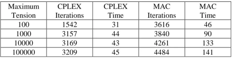
The results of the algorithm for two-piecewise linear costs are compared with the resolution of equivalent linear programs. The software used to solve them was CPLEX 6.0. The time values presented gather both the resolution time of CPLEX and the time needed to generate the linear program. Table 1 shows the evolution of the resolution time when the graph dimension is increasing. Table 2 shows the effect of the tension scale on the resolution time.
Maximum Tension CPLEX Iterations CPLEX Time MAC Iterations MAC Time 100 1542 31 3616 46 1000 3157 44 3840 90 10000 3169 43 4261 133 100000 3209 45 4484 141
Table 2 - Number of Nodes = 500, Number of Arcs = 1000
We can observe that cpu times with the out-of-kilter algorithm are roughly twice bigger than with CPLEX. This is in fact rather encouraging as our method does not include all the heavy data structure machinery which makes CPLEX one of the most efficient LP code on the market. Furthermore, our tool is very flexible and easy to implement into the hypermedia formatter which is far to be the case of CPLEX. Finally, we have shown that our algorithm is able to manage non linear costs functions. We have used CPLEX as a reference to compare optimal solutions of the large-scale graphs and to evaluate the numerical behavior of the proposed algorithm which appears to be quite competitive.
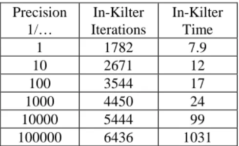
We used the convex function ku
(
θ
u −θ
ˆu)
2on each arc u to test the out-of-kilter method on convex costs. Table 3 shows the evolution of the resolution time when the graph dimension is increasing. Table 4 shows the effect of the precision on the resolution time. We can see that when the precision becomes very small, the time to solve the problem grows exponentially. We suppose that it is partially due to the computer limitation to represent real numbers. However, the number of iterations seems linear when the precision decreases. That means that cycles and cocycles are harder to find when the precision is too small.Number of Nodes Number of Arcs In-Kilter Iterations In-Kilter Time 50 100 846 2.4 50 200 2124 7 50 300 3493 14 50 400 4796 20 50 500 6299 31 100 200 1764 7.7 100 400 4482 24 100 600 7376 53 100 800 10637 95 100 1000 13216 128 500 1000 10627 305 500 2000 28518 1024 500 3000 47612 2078 500 4000 69458 3780 500 5000 60308 1794 1000 2000 22845 1810 1000 4000 62956 1111 1000 6000 105908 1287 1000 8000 156715 1919 1000 10000 195051 1981 Table 3 - Precision = 1/1000
Precision 1/… In-Kilter Iterations In-Kilter Time 1 1782 7.9 10 2671 12 100 3544 17 1000 4450 24 10000 5444 99 100000 6436 1031
Table 4 - Number of Arcs = 100, Number of Nodes = 400
The previous results were obtained on randomly generated graphs. Beside that, we have investigated the class of series-parallel graphs, because they bear many common features with the hypermedia temporal graphs. Indeed, these latter graphs get their particularities from the existence of parallel paths between synchronization nodes and the cycles formed by these paths are nothing but elementary series-parallel graphs. Formally, a series-parallel graph is a graph which cannot be reduced to a complete graph of 4 nodes (the K4 clique). More intuitively, these are the graphs which can be constructed by iterative applications of the two basic operations:
• Sequential splitting: an arc is separated into two consecutive arcs by the introduction of an intermediate node.
• Parallel splitting: an arc is substituted by two parallel arcs with the same end points.
The complete numerical study about the method behavior on these graphs cannot be reproduced here (see [BaHL00]), but the conclusions are quite promising. We understood that the temporal graphs we have to model are some simple extensions of series-parallel graphs. For this kind of graphs, the computational times are distinctly lower (by an order of magnitude) than for general graphs. Moreover, these graphs seem to be easier to solve when discrete objective functions are used. For instance, we may try to minimize the number of objects which have to be moved from their ideal status. This problem is in general an NP-complete problem, which can be approximately solved by relaxation and branch-and-bound methods. However, these approaches are still too time-costly to be useful for decisions at execution time. On the other hand, they can be composed with the continuous cost function when the problem has multiple optimal solutions. That situation typically occurs when the cost is piecewise linear while a unique optimum is obtained with strongly convex functions.
6. Final Remarks
In order to solve the elastic time computation in hypermedia document formatting, we proposed a new algorithm to solve the minimum-cost tension problem. The algorithm appears to be competitive, even when the arc costs are piecewise linear. The distribution of computation among the arcs of a temporal graph turns the approach attractive for the on-the-fly readjustments of the schedule. Even if the introduction of unpredictable events turns the optimization problem helpless, some simulation tools may try to identify the critical sub-paths of the presentation graph.
Series-parallel graphs appear to be a nice tool to help building and optimizing the temporal graphs. These graphs have been widely studied in the graph theory literature [Duff65], but it is, to our knowledge, the first time they are analyzed in this context.
We can now return to the six goals presented in Section 3 to discuss directions for future work. The first goal is an NP-Complete problem, requiring the use of heuristics and approximations, which is a research already under development in our group. However, we are also investigating a polynomial solution using the series-parallel graph approach. With our results we can conclude that the second goal can easily be reached for continuous cost functions. However, for discrete functions it is also an NP-Complete problem that must be investigated. The third goal is naturally reached by our temporal graph, by adding two nodes
N1 and N2 and three arcs: the first linking N1 to N2 and having the desired presentation
duration, and the other two linking the head node to N1 and N2 to the tail node, respectively.
The fourth goal was also solved by our temporal graph. To obtain the minimum and maximum possible duration for a given presentation, the idea is similar to the previous one, but now, instead of fixing the N1 to N2 arc duration, one should set its feasibility as indeterminate. From
our point of view, the fifth and sixth goals present indeed the hardest issues to be solved. As aforementioned, the distribution of computation among the arcs of a temporal graph turns the approach attractive for the on-the-fly schedule readjustments. The problem solution, however, remains as a goal for future work.
References
[Alle83] Allen J. “Maintaining Knowledge About Temporal Intervals”, Communications of the
ACM, vol. 26, no 11, 1983, pp. 832-843.
[AhMO91] Ahuja R.K., Magnanti T.L., Orlin J.B.; “Network Flows”, Prentice-Hall, 1991.
[BeGh62] Berge C., Ghouila-Houri A. “Programmes, Jeux et Réseaux de Transport”, Dunod ed., 1962.
[BaHL00] Bachelet B., Huiban G., Lalande J.F. “Calcul des temps élastiques sur des graphes séries-parallèles”, Res. Rept LIMOS, 2000.
[BuZe93a] Buchanan M.C., Zellweger P.T. “Automatically Generating Consistent Schedules for Multimedia Documents”, Multimedia Systems, Springer-Verlag, 1993.
[BuZe93b] Buchanan M.C., Zellweger P.T. “Automatic Temporal Layout Mechanisms”, ACM
International Conference on Multimedia, California, USA, 1993, pp. 341-350.
[DiSé94] Diaz M., Sénac P. “Time Stream Petri Nets, a Model for Timed Multimedia Information”, Proceedings of the 15th International Conference on Application and Theory of Petri
Nets, Zaragoza, 1994, pp. 219-238.
[Duff65] Duffin R.J. “Topology of series-parallel graphs”, J. Math. Anal. Appll. 10, 1965, pp. 303-318.
[Fulk61] Fulkerson D.R. “An out-of-kilter method for minimal cost flow problems”, SIAM J. on
Applied Math. 9, 1961, pp. 18-27.
[Hadj96] Hadjiat M. “Problèmes de tension sur un graphe – Algorithmes et complexité”, PhD
Thesis, Université de Marseille, 1996.
[KiSo95] Kim M., Song J. “Multimedia Documents with Elastic Time”, Proceedings of ACM
Multimedia’95, San Francisco, USA, November 1995.
[LiGh90] Little T., Ghafoor A. “Synchronization and Storage Models for Multimedia Objects”,
IEEE J. Selected Areas of Commun., vol. 8, no. 3, 1990, pp. 413-427.
[PéLi96] Pérez-Luque M., Little T. “A Temporal Reference Framework for Multimedia Synchronization”, IEEE Journal on Selected Areas in Communications (Special issue:
[Pla71] Pla J.M. “An out-of-kilter algorithm for solving minimum-cost potential problems”,
Mathematical Programming, 1971, pp. 275-290.
[SaLR99] Sabry-Ismail L., Layaïda N., Roisin C. “Dealing with uncertain durations in synchronized multimedia presentations”, Multimedia Tools and Applications Journal, Kluwer Academic Publishers, 1999.
[Soar00] Soares L.F. “Modelo de Contextos Aninhados Versão 2.3”. Technical Report of
TeleMidia Lab, Departamento de Informática, PUC-Rio, Rio de Janeiro, Brazil, January 2000.
[SoRM00] Soares L.F., Rodrigues R., Muchaluat-Saade D. “Authoring and Formatting Hypermedia Documents in the HyperProp System”, to appear in the Special Issue on Multimedia Authoring and
Presentation Techniques of the ACM/Springer-Verlag Multimedia Systems Journal, 2000.
[W3C98] “Synchronized Multimedia Integration Language (SMIL) 1.0 Specification”. W3C