Data-driven optimization and analytics for operations management applications

(1)

Data-driven optimization and analytics for operations

management applications

by

Joline Ann Villaranda Uichanco

Submitted to the Sloan School of Management in partial fulfillment of the requirements for the degree of

Doctor of Philosophy in Operations Research at the

MASSACHUSETTS INSTITUTE OF TECHNOLOGY September 2013

c

Author . . . . Sloan School of Management

August 1, 2013

Certified by . . . . Georgia Perakis William F. Pounds Professor of Management Professor of Operations Research and Operations Management Thesis Supervisor Certified by . . . . Retsef Levi J. Spencer Standish (1945) Professor of Management Associate Professor of Operations Managementat Thesis Supervisor

Accepted by . . . . Dimitris Bertsimas Boeing Professor of Operations Research Co-director, Operations Research Center

(2)

(3)

Data-driven optimization and analytics for operations management applications

by

Joline Ann Villaranda Uichanco

Submitted to the Sloan School of Management on August 1, 2013, in partial fulﬁllment of the

requirements for the degree of

Doctor of Philosophy in Operations Research

Abstract

In this thesis, we study data-driven decision making in operation management contexts, with a focus on both theoretical and practical aspects.

The ﬁrst part of the thesis analyzes the well-known newsvendor model but under the assumption that, even though demand is stochastic, its probability distribution is not part of the input. Instead, the only information available is a set of independent samples drawn from the demand distribution. We analyze the well-known sample average approximation (SAA) approach, and obtain new tight analytical bounds on the accuracy of the SAA solution. Unlike previous work, these bounds match the empirical performance of SAA observed in extensive computational experiments. Our analysis reveals that a distribution’s weighted mean spread (WMS) impacts SAA accuracy. Furthermore, we are able to derive distribution parametric free bound on SAA accuracy for log-concave distributions through an innovative optimization-based analysis which minimizes WMS over the distribution family.

In the second part of the thesis, we use spread information to introduce new families of demand distributions under the minimax regret framework. We propose order policies that require only a distribution’s mean and spread information. These policies have several attractive properties. First, they take the form of simple closed-form expressions. Second, we can quantify an upper bound on the resulting regret. Third, under an environment of high profit margins, they are provably near-optimal under mild technical assumptions on the failure rate of the demand distribution. And finally, the information that they require is easy to estimate with data. We show in extensive numerical simulations that when profit margins are high, even if the information in our policy is estimated from (sometimes few) samples, they often manage to capture at least 99% of the optimal expected profit.

The third part of the thesis describes both applied and analytical work in collaboration with a large multi-state gas utility. We address a major operational resource allocation problem in which some of the jobs are scheduled and known in advance, and some are unpredictable and have to be addressed as they appear. We employ a novel decomposition approach that solves the problem in two phases. The ﬁrst is a job scheduling phase, where regular jobs are scheduled over a time horizon. The second is a crew assignment phase, which assigns jobs to maintenance crews under a stochastic number of future emergencies. We propose heuristics for both phases using linear programming relaxation and list scheduling. Using our models, we develop a decision support tool for the utility which is currently being piloted in one of the company’s sites. Based on the utility’s data, we project that the tool will result in 55% reduction in overtime hours.

Thesis Supervisor: Georgia Perakis

(4)

Professor of Operations Research and Operations Management Thesis Supervisor: Retsef Levi

Title: J. Spencer Standish (1945) Professor of Management Associate Professor of Operations Managementat

(5)

Acknowledgments

There are many people I would like to thank who have helped and supported me in my Ph.D. journey, which culminates with this thesis.

I dedicate this thesis to my mother, Jocelyn, who has sacriﬁced so much throughout the years and who has raised two children despite personal diﬃculties. Without her, I would not be where I am. Through her example, she has taught me tenacity, resilience, and strong values. I also thank my brother, Joseph, who I know I can count on in times of trouble.

I send my heartfelt thanks to my two fantastic research advisors, Retsef and Georgia, who I have known since my Masters program at MIT. I could not have had better advisors. My Ph.D. journey has had many emotional highs and lows which I could not have weathered without them. They have given me mentorship, moral support and encouragement. I also thank my Masters advisors, Karthik Natarajan and Melvyn Sim, who still remain my mentors.

I would like to send special thanks to Steve Graves and Melvyn Sim for participating in my thesis committee.

Thanks to employees at National Grid, whose help was valuable in writing my thesis. Thanks to Mallik Angalakudati, Sid Balwani, Jorge Calzada, Bikram Chatterjee, and Nick Raad.

I thank all the friends that I made throughout the past ﬁve years. I am grateful for the friendship I have found in Ilke Kalcioglu, who has been my roommate for two years and who remains like a sister to me. I thank Ruben Lobel for also being supportive and being such a good friend. Special thanks also goes to Sun Wei, who is also like a sister and who never fails to give advice when I need it.

I thank my good friends, Chaitanya Bandi, Ozan Candogan, Mihalis Markakis, and Yehua Wei, who were in the academic job search with me. I’m glad we went through this process together. I wish them all the best for the future.

I’m grateful for my friends from the ORC. I’m grateful to Ta Chiraphadhanakul, Cristian Figueroa, and Matthieu Monsch for the times we spent studying for Quals, having dinner at Pad Thai Cafe, and watching movies during our ﬁrst few years. Thanks to the rest of my classmates, Dimitrios Bisias, Michael Frankovich, Zach Leung, Xin Lu, Anna Teytelman, Eric Zarybnisky, and Yuan Zhong.

Thanks to Jason Acimovic, Kostas Bimpikis, Shi Cong, Doug Fearing, Dan Iancu, Ilan Lobel, Nikos Trichiakis and Gerry Tsoukalas, who graduated before me but who all have still supported me.

I also thank the friends I made at the ORC, Ross Anderson, Fernanda Bravo, Andre Calmon, Maxime Cohen, Adam Elmachtoub, Matthew Fontana, Paul Grigas, Vishal Gupta, Shubham Gupta, Swati Gupta, Kris Johnson, Nathan Kallus, Phil Keller, John Kessler, Jonathan Kluberg, Angie King, Maokai Lin, Will Ma, Allison O’Hair, Eric Robinson, Joel Tay, Leon Valdes, and Nataly Youssef. I’m glad for all the memories we’ve made throughout

(6)

the years of INFORMS, ISMP and MSOM trips, of barbecues, parties and concerts, of camping trips, of C-Functions, of Thirsty Ear karaoke nights, and of many others.

Thanks to my friends outside of the ORC, who have shared experiences with me and who have also been good emotional support. Thanks to Burak Alver, Doug Clendenin, Laura Kligler, Roza Mahmoodian, Karen Nadua, Ferron Ocampo, Nestor Precioso, Nikolas Pyrgiotis, Val San Antonio, Yannis Simiakis, and Melis Tanner, and Derek Yao.

Finally, I am grateful for the ORC Co-directors, Dimitris Bertsimas and Patrik Jaillet, who have truly been committed to the welfare of the students and the Center. Also, thanks to the amazing ORC administrative staﬀ, Andrew Carvalho, Paulette Mosley, and Laura Rose.

(7)

List of Figures

2-1 The intervals S_ϵLRS and Sϵf of a newsvendor cost function C. . . . 24

2-2 Probability density function and cost function (b = 5, h = 5) for a uniform and normal distribution. . . 29 2-3 Marginal beneﬁt of additional data as a function of the sample size. . . 37 3-1 Regret function under a normal and a uniform distribution when β = 0.5. 48 3-2 Actual relative regret of partial information policies plotted against the proﬁt

margin β. . . . 50 3-3 Actual relative regret of partial information policies plotted against the proﬁt

margin β. . . . 51 4-1 Historical distribution of the number of emergencies in a given yard for April. 71 4-2 Current system: Actual crew-hours worked in April 2011 in an average-sized

yard. . . 73 4-3 Relative MIP gap in Gurobi’s branch and bound. . . 77 4-4 Cost diﬀerence between rolling horizon job scheduling model and perfect

hindsight model. . . 83 4-5 An example of a dynamic assignment . . . 90 4-6 Overtime hours saved by dynamic reassignment . . . 90 4-7 Hypothetical scenario: Crew-hours worked if optimization model is used to

schedule jobs. . . 92 4-8 Workable jobs queue over one simulated month with 50% service level. . . 94 C-1 Upper bound for a log-concave distribution with _b+hb quantile q∗. . . 130 C-2 Regression analysis to estimate relationship between bias of ∆n and AMS

value ∆F(β). . . . 130

C-3 Probability density functions of demand distributions used in experiments. 131 C-4 Probability density functions of demand distributions used in experiments. 132

(12)

(13)

List of Tables

2.1 Theoretical bounds and actual empirical performance of SAA. . . 26

2.2 Regression analysis of ϵ = CNk . . . 30

2.3 Regression analysis of ϵ = C{∆(q∗)f (q∗)}k . . . 31

2.4 Sample size equating marginal cost to estimated marginal beneﬁt of addi-tional sample. . . 36

3.1 Fraction (%) of sample-based conﬁdence intervals that contain the true spread. . . . 57

3.2 Average relative regret (%) of policies using sample estimates of AMS infor-mation. . . 59

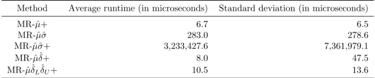
3.3 Average run times of each method . . . 61

3.4 Average relative regret (%) of policies using sample estimates of information under high proﬁt margins (β = 0.9, 0.95). . . . 62

3.5 Average relative regret (%) of policies using sample estimates of information under extremely high proﬁt margins (β = 0.99, 0.995). . . . 63

3.6 Maximum regret achieved by SAA policy out of familyDµ,δ,+, which includes the distribution used to generate the samples. . . 64

4.2 Maximum work hours in diﬀerent scenarios under optimal assignment and assignment based on average number of leaks. . . 85

4.3 Expected maximum hours worked under the optimal crew assignment and the assignment from Algorithm Stoch-LPT. . . 87

4.4 Eﬀect of service levels on average workable jobs inventory, backlogged jobs, and overtime crew-hours for one simulated month. . . 94

4.5 Total expected overtime crew-hours for diﬀerent expertise factors. . . 95

4.6 Simulation results for increasing supervisor presence in the ﬁeld. . . 97

4.7 Projected ﬁnancial impact of business process changes in a hypothetical util-ity with a $3.5 billion annual operating proﬁt. . . 98

D.1 Range of critical fractile values where Assumption 2.4.1 holds. . . 134

D.2 Average errors (%) with samples from an exponential distribution. . . 134

(14)

D.4 Average errors (%) with samples from a Pareto distribution. . . 135

D.5 Average errors (%) with samples from a Beta distribution. . . 136

D.6 Average errors (%) with samples from a mixed normal distribution. . . 136

D.7 Regression analysis to estimate relationship between bias of ∆n and sample size n. . . . 137

D.8 Theorem 3.2.2: Optimal primal and dual solutions when z≤ y ≤ w . . . . 137

D.9 Theorem 3.2.2: Optimal primal and dual solutions when z≤ w ≤ y . . . . 137

D.10 Theorem 3.2.2: Optimal primal and dual solutions when y≤ z ≤ w . . . . 138

D.11 Theorem 3.2.2: Optimal primal and dual solutions when y≤ w ≤ z . . . . 138

D.12 Theorem 3.2.2: Optimal primal and dual solutions when w≤ z ≤ y . . . . 138

D.13 Theorem 3.2.2: Optimal primal and dual solutions when w≤ y ≤ z . . . . 139

D.14 Theorem 3.2.2: G(z; y) . . . 139

D.15 Theorem A.3.1: Optimal primal and dual solutions when z≤ y ≤ w . . . . 140

D.16 Theorem A.3.1: Optimal primal and dual solutions when z≤ w ≤ y . . . . 140

D.17 Theorem A.3.1: Optimal primal and dual solutions when y≤ z ≤ w . . . . 141

D.18 Theorem A.3.1: Optimal primal and dual solutions when y≤ w ≤ z . . . . 142

D.19 Theorem A.3.1: Optimal primal and dual solutions when w≤ z ≤ y . . . . 143

D.20 Theorem A.3.1: Primal and dual solutions when w≤ y ≤ z . . . 143

D.21 Theorem A.3.1: G(z; y) when µ− (1 − β)δU < 0 . . . 144

D.22 Theorem A.3.1: G(z; y) when µ− (1 − β)δU ≥ 0 . . . 145

D.23 Durations of standard jobs. . . 146

D.24 Probability distributions of number of gas leaks. . . 146

D.25 Optimal crew assignment with leak distribution 1. . . 147

D.32 Crew assignment using Algorithm Stoch-LPT with leak distribution 1. . . 154

(15)

Chapter 1

Introduction

In managing the operations of a ﬁrm, decisions often have to be made in an environment having some underlying uncertainty. Some examples include inventory management, supply chain coordination, revenue management, and workforce management. In this thesis, we discuss decision making in operations management contexts under uncertainty, with a focus on both theoretical and practical aspects.

In the ﬁrst part of the thesis, we make the assumption that the probability distribution of the underlying uncertainty is not known as part of the input. This is particularly relevant in real-world applications since the decision maker does not have a complete description of the underlying uncertainty.

In Chapter 2, we consider the well-known newsvendor model, however the only infor-mation available is a set of independent samples drawn from the demand distribution. We consider the well-known sample average approximation (SAA) approach, but there is a cost associated with the sampling process. Gathering more samples incurs a sampling cost. On the other hand, gathering less samples incurs an inaccuracy cost. The sample size must be carefully chosen to balance the cost tradeoﬀs involved with sampling. We model inaccuracy cost as the expected penalty, where a ﬁxed penalty is incurred in the event that the relative regret of the SAA quantity exceeds a threshold. We obtain new tight analytical bounds on the probability of this event which match the empirical performance observed in ex-tensive computational experiments. Unlike previous work, this bound reveals the weighted

mean spread (WMS) as an underlying property of the demand distribution which impacts

the accuracy of the SAA procedure. Furthermore, we are able to derive a bound indepen-dent of distribution parameters based on an innovative optimization-based analysis which minimizes WMS over a distribution family.

In Chapter 3, we study a minimax regret approach to the newsvendor problem. Using a distribution statistic, called absolute mean spread (AMS), we introduce new families of demand distributions under the minimax regret framework. We propose order policies that require only a distribution’s mean and information on the AMS. Our policies have several attractive properties. First, they take the form of simple closed-form expressions. Second,

(16)

we can quantify an upper bound on the resulting regret. Third, under an environment of high profit margins, they are provably near-optimal under mild technical assumptions on the failure rate of the demand distribution. And finally, the information that they require is easy to estimate with data. We show in extensive numerical simulations that when profit margins are high, even if the information in our policy is estimated from (sometimes few) samples, they often manage to capture at least 99% of the optimal expected profit.

In the second part of the thesis, we demonstrate using a real-world example how analytics and optimization is used for decision-making in a gas utility.

In Chapter 4, we describe a project which addresses a major operational resource allo-cation challenge that is typical to the industry and to other appliallo-cation domains. We study the resource allocation problem in which some of the tasks are scheduled and known in advance, and some are unpredictable and have to be addressed as they appear. The utility company has maintenance crews that perform both standard jobs (each must be done before a speciﬁed deadline) as well as repair emergency gas leaks (that occur randomly throughout the day, and could disrupt the schedule and lead to signiﬁcant overtime). The goal is to perform all the standard jobs by their respective deadlines, to address all emergency jobs in a timely manner, and to minimize maintenance crew overtime.

We employ a novel decomposition approach that solves the problem in two phases. The ﬁrst is a job scheduling phase, where standard jobs are scheduled over a time horizon. The second is a crew assignment phase, which solves a stochastic mixed integer program to assign jobs to maintenance crews under a stochastic number of future emergencies. For the ﬁrst phase, we propose a heuristic based on the rounding of a linear programming relaxation formulation and prove an analytical worst-case performance guarantee. For the second phase, we propose an algorithm for assigning crews to replicate the optimal solution structure.

We used our models and heuristics to develop a decision support tool for the utility which is currently being piloted in one of the company’s sites. Using the utility’s data, we project that the tool will result in 55% reduction in overtime hours.

(17)

Chapter 2

The data-driven newsvendor

2.1 Introduction

In the classical newsvendor problem, a retailer plans to sell a product over a single period to meet a stochastic demand with a known distribution (Zipkin, 2000). She needs to commit to a stocking quantity before observing the actual demand at the end of the sales period. The retailer incurs an underage cost for each unit of unsatisﬁed demand, and an overage

cost for each unsold unit of product at the end of the period. The goal of the retailer is to

choose an order quantity that minimizes the expected cost. The basic assumption of the newsvendor model is that the demand distribution is known.

In reality, managers need to make inventory decisions without having complete knowl-edge of the demand distribution. Often, the only information available comes from a set of demand data. Nonparametric data-driven heuristics are a class of heuristics that as-sume the demand data is a random sample drawn from the unknown demand distribution. Typically, these data-driven heuristics are more accurate as the sample size increases. If there is no cost incurred for gathering samples, then it is better to gather as many demand samples as possible. However, in some realistic settings, there is a cost associated with the

data-collection or sampling process. Gathering more samples incurs a sampling cost. On

the other hand, gathering less samples incurs an inaccuracy cost. The sample size must be carefully chosen to balance the cost tradeoﬀs involved with sampling. In this chapter, we analyze the cost tradeoﬀs under the popular nonparametric data-driven heuristic called

sample average approximation (SAA) (Homem-De-Mello, 2000; Kleywegt et al., 2001). The

SAA heuristic minimizes the cost averaged over the empirical distribution induced by the sample, instead of the true expected cost that cannot be evaluated.

In our model, let D be the stochastic single-period demand. Let C(q) denote the ex-pected underage and overage cost of an inventory level q. If the true distribution of D is known, then the optimal newsvendor quantity q∗= minq≥0C(q) is a well-speciﬁed quantile

of the distribution (sometimes called the critical quantile). In our setting, the distribution of D is unknown, but a random sample of size N drawn from the unknown distribution is

(18)

available. Let ˆQN denote the SAA solution, which is stochastic since its value depends on

the random sample. We assess the accuracy of the SAA solution by comparing its expected cost C( ˆQN) against the optimal expected cost C(q∗). The diﬀerence, C( ˆQN)− C(q∗), is

often called the error (or the regret ) of ordering the SAA solution. The regret normalized by C(q∗) is referred to as the relative regret.

Let θS(N ) denote the sampling cost of a sample of size N . For instance, θS(N ) may

be linear and increasing in the sample size: θS(N ) = ρN , where ρ > 0 is the cost

in-curred for each demand data. Let θI(N ) denote the inaccuracy cost of the SAA solution.

There are multiple ways to deﬁne the inaccuracy cost θI depending on the speciﬁc problem

context. Suppose a penalty K is incurred whenever the relative regret of the SAA solu-tion exceeds a speciﬁed threshold ϵ. In this chapter, we choose to model the inaccuracy cost of sampling as the expected penalty incurred by ordering the SAA solution. That is,

θI(N ), E ( K· 1_[_{C( ˆ}_Q N)>(1+ϵ)C(q∗)] ) = K· Pr ( C( ˆQN) > (1 + ϵ)C(q∗) )

, where 1[A] is the indicator function of event A; it takes a value of 1 if event A occurs and zero otherwise.

The optimal choice of the sample size N minimizes the total cost θS(N )+θI(N ). Solving

this requires evaluating θI or, equivalently, having a probabilistic understanding of the

relative regret of the SAA heuristic, (C( ˆQN)−C(q∗))/C(q∗), as a function of the sample size.

In this work, we provide an entirely new optimization-based analysis that: (i) Obtains tight analytical probabilistic bounds on SAA accuracy that match the empirical performance. As a result they can be used to accurately estimate the value of additional samples; and (ii) Highlights several new important properties of the underlying demand distribution that drive the accuracy of the SAA heuristic.

2.1.1 Contributions and Insights

Our work has multifold contributions and provides several important insights:

Informative probabilistic bound. We derive a new analytical bound on the

proba-bility that the SAA solution has at most ϵ relative regret. This bound depends only on the sample size, the threshold ϵ, the underage and overage cost parameters, as well as a newly introduced property of the demand distribution called weighted mean spread (WMS). To the best of our knowledge, the WMS is an entirely new concept first introduced in this thesis. The absolute mean spread (AMS) at x, ∆(x), is the difference between the conditional ex-pectation of demand above x and the conditional exex-pectation below the x (Definition 2.4.1). The WMS at x is simply the AMS weighted by the density function value, i.e. ∆(x)f (x). Our analysis shows that the WMS is the property that drives the accuracy of the SAA method. Specifically, the probability that the SAA solution has a relative regret greater than ϵ decays exponentially with a constant proportional to ∆(q∗)f (q∗). Thus, the SAA procedure is more likely to be have smaller regret if samples are drawn from a distribution with a large value for ∆(q∗)f (q∗).

Tight probabilistic bounds. Regression analysis demonstrates that the probabilistic

(19)

quantify the accuracy gained from obtaining additional samples. This is especially valuable in settings where data-collection incurs a cost. Thus, we are able to characterize the optimal sample size that balances the sampling cost and inaccuracy cost.

Probabilistic bounds for log-concave distributions. The new notion of WMS is used to develop a general optimization-based methodology to derive tight probabilistic bounds for the accuracy of the SAA method over any nonparametric family of distributions. This is done through a specified optimization problem that minimizes the WMS, ∆(q∗)f (q∗), over the family of distributions. We are able to solve this problem in closed form for the important family of log-concave distributions, providing a tight lower bound on ∆(q∗)f (q∗) of all log-concave distributions. As a consequence, we obtain a uniform probabilistic bound for the accuracy of the SAA solution under any log-concave demand distribution. This bound is independent of distribution-specific parameters, and only depends on the sample size, the regret threshold, and the underage and overage cost parameters. (Note that many of the common distributions assumed in inventory and operations management are log-concave, e.g., normal, uniform, exponential, logistic, chi-square, chi, beta and gamma distributions.) The new bound is significantly tighter than the bound in Levi et al. (2007). The methodology we developed could potentially be used to derive probabilistic bounds for SAA accuracy under other distribution families. We believe this is a promising future research direction.

Comparing SAA vs. traditional fitting approaches. Finally, we conduct an extensive computational study comparing the accuracy of the SAA method against the naive (but commonly used in industry) approach that first fits the samples to a specified distribution and then solves the newsvendor problem with respect to that distribution. The comparison is made based on the average relative regret each method incurs. To implement the fitting approach, we used the distribution-fitting software EasyFit to find the distribution that best describes the samples from its database of more than 50 distributions. We investigate the effect of the sample size and the effect of sampling from nonstandard demand distributions on the magnitude of the relative regret. In most cases, even when the critical quantile is high, the errors of the SAA method are on par or dominate those of the distribution fitting approach. Moreover, when the samples are drawn from a nonstandard distribution (e.g., mixed normals), the distribution fitting method results in huge errors compared to the SAA method.

2.1.2 Literature Review

There exists a large body of literature on models and heuristics for inventory problems that can be applied when limited demand information is known. One may use either a

paramet-ric approach or a nonparametparamet-ric approach. A parametparamet-ric approach assumes that the true

distribution belongs to a parametric family of distributions, but the speciﬁc values of the parameters are unknown. In contrast, a nonparametric approach requires no assumptions regarding the parametric form of the demand distribution. The following are some

(20)

exam-ples of parametric approaches. Scarf (1959) proposed a Bayesian procedure that updates the belief regarding the uncertainty of the parameter based on observations that are col-lected over time. More recently, Liyanage & Shanthikumar (2005) introduced operational

statistics which, unlike the Bayesian approach, does not assume any prior knowledge on

the parameter values. Instead it performs optimization and estimation simultaneously. In another recent work, Akcay et al. (2009) propose fitting the samples to a distribution in the Johnson Translation System, which is a parametric family that includes many common distributions. Besides SAA, the following are other examples of nonparametric approaches proposed in previous work. Concave adaptive value estimation (CAVE) (Godfrey & Powell, 2001) successively approximates the objective cost function with a sequence of piecewise linear functions. The bootstrap method (Bookbinder & Lordahl, 1989) estimates the crit-ical quantile of the demand distribution. The infinitesimal perturbation approach (IPA) is a sampling-based stochastic gradient estimation technique that has been used to solve stochastic supply chain models (Glasserman & Ho, 1991). Huh & Rusmevichientong (2009) develop an online algorithm for the newsvendor problem with censored demand data (i.e., data is on sales instead of demand) based on stochastic gradient descent. Another nonpara-metric method for censored demand is proposed by Huh et al. (2008), based on the well-known Kaplan-Meier estimator. Robust optimization addresses distribution uncertainty by providing solutions that are robust against different distribution scenarios. It does this by allowing the distribution to belong to a specified family of distributions. Then one can use a max-min approach, attempting to maximize the worst-case expected profit over the set of allowed distributions. Scarf (1958) and Gallego & Moon (1993) derived the max-min order policy for the newsvendor model with respect to a family of distributions with the same mean and variance. Another robust approach attempts to minimize the worst-case “regret” (or hindsight cost of suboptimal decision) over the distribution family. Some recent works using a minimax regret criterion include Ball & Queyranne (2009); Eren & Maglaras (2006); Perakis & Roels (2008); Levi et al. (2013b).

In general, the sample average approximation (SAA) method is used to solve two types of stochastic optimization problems. The first type of problems are those that are computa-tionally difficult even though the underlying distribution is known (e.g. two-stage discrete problems where the expectation is difficult to evaluate due to complicated utility functions and multivariate continuous distributions). In this case, sampling is used to approximate the complicated (but known) objective function. The resulting sample approximation leads to a deterministic equivalent problem (e.g. an integer program) that is finite, though pos-sibly with a large dimension due to the number of samples. Some analytical results about probabilistic bounds for SAA accuracy have been derived for two-stage stochastic integer programs (Kleywegt et al., 2001; Swamy & Shmoys, 2005; Shapiro, 2008). It was shown by Kleywegt et al. (2001) that the optimal solution of the SAA problem converges to the true optimal value with probability 1. They also derive a probabilistic bound on the SAA accuracy that depends on the variability of the objective function and the size of the feasible

(21)

region, however they observe it to be too conservative for practical estimates. In this ﬁrst type of problems, understanding the accuracy of SAA is importance since the sample size directly inﬂuences the computational complexity of the problem.

The second type of problems SAA is used to solve are problems whose objective functions are easy to evaluate if the distribution is known (like for the newsvendor problem), however the complication is that the distribution is unknown. Sampling is used to estimate the unknown distribution. The problem we are dealing with in this chapter falls under this second category of problems. If there is an explicit cost for sampling, the accuracy of the SAA solution as a function of the sample size needs to be understood to determine the tradeoff between sampling cost and inaccuracy cost. The accuracy of the SAA solution for the newsvendor problem is analyzed by Levi et al. (2007) who derive a probabilistic bound on its relative regret. This probabilistic bound is independent of the underlying demand distribution, and only depends on the sample size, the error threshold, and the overage and underage cost parameters. Since it applies to any demand distribution, it is uninformative and highly conservative. It is uninformative since it does not reveal the types of distributions for which the SAA procedure is likely to be accurate. It is conservative because, as we demonstrate in computational experiments later in this chapter, the probabilistic bound in Levi et al. (2007) does not match the empirical accuracy of the SAA seen for many common distributions. Since it is not tight, this probabilistic bound is of limited value in a setting where data-collection incurs a cost. We show later in Section 2.6 that the analysis of Levi et al. (2007) greatly underestimates the benefit of gathering additional samples. Similar to the probabilistic bounds derived for the first type of problems using SAA, our probabilistic bounds are distribution-specific. However, unlike those bounds, our bounds are tight. Since the demand distribution is unknown, we use an optimization-based framework to derive probabilistic bounds for SAA accuracy that do not depend on any distribution-parameters.

Other works have analyzed the regret of a nonparametric data-driven heuristic under

censored demand data. When data is censored, the choice of the inventory level aﬀects the

demand data for the next period. Thus, the problem of choosing inventory levels is an online convex optimization problem, because the objective function is not known, but an iterative selection of a feasible solution yields some pertinent information. Since the choice of the current period’s solution inﬂuences the next period’s information, the choice of the sample size is not the critical factor; rather, the critical issue is the design of an online policy to ensure that the regret diminishes over time. Recent results in online convex optimiza-tion propose algorithms with convergence of O(1/√N ) for the expected regret averaged

over N periods for perishable inventory (Flaxman et al., 2005). Huh & Rusmevichientong (2009) propose an online algorithm for nonperishable inventory which achieves the same convergence rate. The convergence rate can be improved to O(log(N + 1)/N ) when the probability density function f has a nonzero lower bound on an interval containing q∗ (Huh & Rusmevichientong, 2009). In contrast with these works, the focus of our chapter is on

(22)

the case of uncensored demand. Therefore, since the choice of the inventory level does not aﬀect the next period’s data, the accuracy of the heuristic only depends on the regret of the current period. Moreover, the focus of our chapter is bounding the probability that the

relative regret exceeds a small threshold, rather than the more conservative expected relative

regret criterion. Finally, we observe if we were concerned with the regret (rather than the

relative regret) of the SAA solution, then the probability bound on the SAA solution having

regret exceeding ϵ decays exponentially with a constant proportional to f (q∗). Therefore, as with Huh & Rusmevichientong (2009), if a nonzero lower bound on f (q∗) exits, then a probability bound independent of the distribution can be derived. However, since our chapter is concerned with relative regret, the probability bound decays with a constant of ∆(q∗)f (q∗). As we show in the chapter, the task of ﬁnding a uniform lower bound for ∆(q∗)f (q∗) is achievable for the class of log-concave distributions.

Finally, our results are also related to quantile estimation literature. This is because the SAA solution for the newsvendor problem is a particular sample quantile of the empirical distribution formed by the demand samples. The confidence interval for the quantile esti-mator are well-known (Asmussen & Glynn, 2007). However, unlike in quantile estimation, the accuracy of the SAA solution does not depend on the absolute difference between the true quantile and the quantile estimator. Rather it depends on the cost difference between the true quantile and the estimator Thus, in our work, we find a relationship between the two types of accuracies.

2.1.3 Outline

This chapter is structured as follows. In §2.2, we describe the data-driven single-period newsvendor problem. We also discuss a general setting where data-collection incurs a cost linear in the sample size. §2.3 brieﬂy discusses the analysis of Levi et al. (2007). §2.4 contains the main theoretical contributions of this work. In §2.6, we revisit the problem of choosing a sample size to balance the marginal cost and beneﬁt of sampling. Finally, in§2.7, we perform computational experiments that compare the performance of the SAA approach to other heuristic methods. Unless given, the proofs are provided in Appendix B.

2.2 The Data-driven Newsvendor Problem

In the newsvendor model, a retailer has to satisfy a stochastic demand D for a single product over a single sales period. Prior to observing the demand, the retailer needs to decide how many units q of the product to stock. Only then is demand realized and fulﬁlled to the maximum extent possible from the inventory on hand. At the end of the period, cost is incurred; speciﬁcally, a per-unit underage cost b > 0 for each unit of unmet demand, and a per-unit overage cost h > 0 for each unsold product unit. The goal of the newsvendor is to minimize the total expected cost. That is,

min

q≥0 C(q), E

[

(23)

where x+, max(0, x). The expectation is taken with respect to the stochastic demand D, which has a cumulative distribution function (cdf) F .

Much is known about the newsvendor objective function and its optimal solution (see Zipkin 2000). In particular, C is convex in q with a right-sided derivative ∂+C(q) = −b +

(b + h)F (q) and a left-sided derivative ∂₋C(q) = −b + (b + h) Pr(D < q). The optimal

solution can be characterized through ﬁrst-order conditions. In particular, if ∂₋C(q) ≤ 0

and ∂+C(q)≥ 0, then zero is a subgradient, implying that q is optimal (Rockafellar, 1972).

These conditions are met by

q∗ , inf { q : F (q)≥ b b + h } ,

which is the _b+hb quantile of D, also called the critical quantile or the newsvendor quantile. The basic assumption of the newsvendor problem is that there is access to complete knowledge of F . If the cdf F of the demand is unknown, then the optimal ordering quantity

q∗ cannot be evaluated. Let {D1, D2, . . . , DN} be a random sample of size N drawn from

the true demand distribution, and let{d1, d2, . . . , dN} be a particular realization. Instead of

optimizing the unknown expected cost, the SAA method optimizes the cost averaged over the drawn sample:

min q≥0 ˆ CN(q), 1 N N ∑ k=1 ( b(dk− q)++ h(q− dk)+ ) . (2.1)

Based on the particular sample, the empirical distribution is formed by putting a weight of _N1 on each of the demand values. Note the function ˆCN is the expected cost with respect to

the empirical distribution. Hence, the optimal solution to (2.1) is the _b+hb sample quantile. Formally, we denote the empirical cdf as ˆFN(q) , _N1

∑N

k=11_[Dk_≤q_{]. Let} QˆN denote the

optimal solution to the SAA counterpart with a sample of size N . Thus, ˆQN is the _b+hb

quantile of the random sample: ˆ QN , inf { q : ˆFN(q)≥ b b + h } . (2.2)

Note that ˆQN is a random variable since its value depends on the particular realization of

the random sample.

The SAA procedure is more accurate if the sample size N is large. With a larger sample size, the _b+hb sample quantile, ˆQN, is a closer approximation to the true _b+hb quantile, q∗.

However, we consider in this work the setting where there is a tradeoﬀ between having too few samples and too many samples. Thus, the choice of the sample size needs to be made carefully. In particular, for some constant ρ > 0, we denote by θS(N ) = ρN the

sampling cost incurred from choosing a sample size N . We denote by θI(N ) the inaccuracy

cost incurred from a sample size N , where θI(N ) = K · Pr

(

C( ˆQN) > (1 + ϵ)C(q∗)

) for some ϵ > 0. Note that θI represents the expected penalty from ordering the SAA solution

(24)

Figure 2-1: The intervals S_ϵLRS and Sϵf of a newsvendor cost function C. C S S ε ε LRS q (1+ε)C(q*) C C ~ S S ε ε f q q − − q (1+ε)C(q*)

Note: S_ϵLRS is deﬁned in (2.3); Sϵf will be deﬁned in Section 4 in (2.6)

if a penalty of K is incurred whenever the relative regret of the SAA solution exceeds a threshold ϵ. We are interested in ﬁnding the sample size N for which θS(N ) + θI(N ) is

minimized. This can only be accomplished by developing a probabilistic understanding of how the relative regret of the SAA solution, (C( ˆQN)− C(q∗))/C(q∗), is inﬂuenced by the

sample size. In the next section, we discuss a probabilistic bound due to Levi et al. (2007). Sections 2.4 and 2.5, we introduce a novel asymptotic analysis of the SAA procedure which results in a tighter probabilistic bound. Armed with this analysis, we will again revisit the problem of sample size selection in Section 2.6.

2.3 Distribution-Free Uniform Probability Bounds

As a background for the new analysis discussed in Section 2.4, the bound of Levi et al. (2007) (referred to as the LRS bound) will be discussed ﬁrst. As part of the discussion, it will be shown that in fact their bound can be improved.

The SAA solution is called ϵ-optimal if its relative regret is no more than ϵ. Let us denote the interval consisting of all ϵ-optimal quantities as Sϵ, where Sϵ, {q : C(q) ≤ (1+ϵ)C(q∗)}

(see Figure 2-1). Levi et al. (2007) use the left and right one-sided derivatives of C, denoted by ∂₋C and ∂+C, to deﬁne the following interval:

S_ϵLRS , { q : ∂₋C(q)≤ ϵ 3min(b, h) and ∂+C(q)≥ − ϵ 3min(b, h) } , (2.3)

and then show that S_ϵLRS ⊆ Sϵ (see left plot of Figure 2-1). Note that SϵLRS consists of all

points for which there exists a subgradient with magnitude bounded by ₃ϵmin(b, h). Using large deviations results, specifically the Hoeffding inequality (Hoeffding, 1963), Levi et al. (2007) derive a bound on the probability that the SAA solution ˆQN solved with

(25)

depends on N , γ, and the cost parameters b and h. Note that when γ = ϵ₃min(b, h), the property is equivalent to ˆQN ∈ SϵLRS. Then using the fact that SϵLRS ⊆ Sϵ, they obtain the

following theorem.

Theorem 2.3.1 (LRS bound (Levi et al., 2007)). Consider the newsvendor problem with

underage cost b > 0 and overage cost h > 0. Let ˆQN be the SAA solution (2.2) with sample

size N . For a given ϵ > 0, ˆQN ∈ SϵLRS and C( ˆQN)≤ (1 + ϵ)C(q∗) with probability at least

1− 2 exp ( −2 9N ϵ 2 ( min{b, h} b + h )2) . (2.4)

By using the Bernstein inequality (Bernstein, 1927), we are able to prove a tighter bound than (2.4). Unlike the Hoeﬀding inequality, the Bernstein inequality uses the fact that we seek to estimate the speciﬁc _b+hb quantile. The proof is provided in Appendix B.

Theorem 2.3.2 (Improved LRS bound). Consider the newsvendor problem with underage

cost b > 0 and overage cost h > 0. Let ˆQN be the SAA solution (2.2) with sample size N .

For a given ϵ > 0, ˆQN ∈ SϵLRS and C( ˆQN)≤ (1 + ϵ)C(q∗) with probability at least

1− 2 exp ( − N ϵ2 18 + 8ϵ · min{b, h} b + h ) . (2.5)

The improved LRS bound (2.5) depends on min(b,h)_b+h rather than on (

min(b,h)

b+h

)2 . This is signiﬁcant because in many important inventory systems, the newsvendor quantile _b+hb is typically close to 1, reﬂecting high service level requirements. Thus, _b+hh is close to zero, resulting in a very small value for min(b,h)_b+h . Hence, the improved LRS bound gives a

significantly tighter bound on probability of an ϵ-optimal SAA solution. As an illustration,

consider the SAA method applied to a newsvendor problem in which the service level increases from 95% to 99%. In order to maintain the likelihood of achieving the same accuracy, the LRS bound suggests that the sample size needs to be increased by 25 times. In contrast, the improved LRS bound suggests that the accuracy is maintained by a sample size that is only ﬁve times as large.

The analysis of Levi et al. (2007) yields a probability bound that is general, since it applies to any demand distribution. However, it is uninformative in that it does not shed light on relationship between the accuracy of the SAA heuristic and the particular demand distribution. Furthermore, the LRS bound is very conservative. We demonstrate this empirically through the following experiment. Draw 1000 random samples, each with a sample size of N = 100, from a particular distribution. The respective SAA solutions

{ˆq1

100, . . . , ˆq1001000} are computed, where ˆq100i is the SAA solution corresponding to random sample i. We note that although the samples are drawn from speciﬁc distributions, the SAA solution is computed purely based on the resulting empirical distribution. The respective

(26)

Table 2.1: Theoretical bounds and actual empirical performance of SAA.

Distribution ϵ = 0.02 ϵ = 0.04 ϵ = 0.06 ϵ = 0.08 ϵ = 0.10

Uniform Emp conf 81.8% 93.7% 96.6% 99.0% 98.9%

(A = 0, B = 100) NLRS 1,088,200 395,900 209,200 154,300 97,800

Nf 956 692 544 428 416

Normal Emp conf 75.8% 89.7% 94.7% 97.3% 99.4%

(µ = 100, σ = 50) NLRS 958,830 339,630 186,370 125,390 109,210

Nf 3,812 2,676 2,184 1,940 2,096

Exponential Emp conf 69.6% 84.4% 91.5% 94.0% 98.2%

(µ = 100) NLRS 855,280 292,090 162,120 102,130 88,560

Nf 1,472 996 824 684 736

Lognormal Emp conf 75.1% 90.5% 96.5% 98.2% 98.7%

(µ = 1, σ = 1.805) NLRS 945,890 348,880 207,670 137,190 94,680

Nf 1,272 932 824 720 616

Pareto Emp conf 79.1% 92.6% 98.0% 98.1% 99.5%

(xm= 1, α = 1.5) NLRS 1,025,400 377,500 236,400 135,600 112,600

Nf 1,152 840 780 592 612

a_{“Emp conf” refers to the empirical conﬁdence, or the fraction of random samples where}

the SAA procedure achieves relative regret less than ϵ.

relative regret of the SAA solutions are{ϵ1, . . . , ϵ1000} where ϵi , C(ˆqi100)−C(q∗)

C(q∗) . We refer to the fraction of sets that achieve a relative regret less than the target ϵ to be the empirical

confidence. Using Theorem 2.3.1, we can calculate the minimum sample size predicted

by the LRS bound to match the empirical confidence level. If this LRS sample size is significantly greater than 100, then this would imply that the LRS bound is very loose (i.e., conservative) since the same accuracy and confidence probability can be achieved with a smaller number of samples.

Table 2.1 summarizes the results of the outlined experiment for a newsvendor critical quantile of 0.9. Rows labeled NLRS correspond to the LRS sample size. One can see from

the table that if, for example, the SAA counterpart is solved with samples drawn from a uniform distribution, the relative errors are less than 0.02 in 81.8% of the sets. However, to match this same error and conﬁdence level, the LRS bound requires 1,088,200 samples. This is almost a thousand times as many samples as the 100 used to generate this conﬁdence probability. We can observe that this large mismatch between the empirical SAA accuracy and the theoretical guarantee by the LRS bound prevails throughout various target errors

ϵ and distributions.

One way to understand why the LRS bound is conservative is to observe that the interval

S_ϵLRS is typically very small relative to Sϵ (see the left plot of Figure 2-1). Naturally, the

probability of the SAA solution falling within S_ϵLRS can be signiﬁcantly smaller than the probability of it falling within the larger interval Sϵ.

(27)

2.4 New Approximation to the S

ϵ

Interval

In this section, we shall develop a tighter approximation of Sϵ. Speciﬁcally, we develop an

informative probabilistic bound on the relative regret of the SAA solution that identiﬁes the important properties of the underlying demand distribution that determine the procedure’s accuracy.

Suppose the demand is a continuous random variable with a probability density function (pdf) f , which we assume to be continuous everywhere. (Later in §5, we will show that this assumption is automatically satisﬁed under some simple conditions.) Let ˜C be the

second-order Taylor series approximation of C at the point q = q∗, where q∗ is the optimal newsvendor quantile. Note that since a pdf exists, the cost function is twice diﬀerentiable. It is straightforward to verify that

˜ C(q), bh b + h∆(q ∗_{) +}1 2(b + h)(q− q ∗₎2_{f (q}∗_), where ∆ is the absolute mean spread operator deﬁned below.

Deﬁnition 2.4.1 (Absolute Mean Spread (AMS)). Let D be a random variable. We

define the absolute mean spread (AMS) at x as ∆(x), E(D|D ≥ x) − E(D|D ≤ x).

Observe that ∆(q∗) is simply equal to b+h_bh C(q∗). Consider an approximation to Sϵ using

a sublevel set of ˜C (see the right plot of Figure 2-1): Sf_ϵ ,

{

q : ˜C(q)≤ (1 + ϵ) ˜C(q∗) }

. (2.6)

The superscript f is to emphasize that the interval is deﬁned by the particular distribution

f . The two endpoints of Sϵf are:

q, q∗− √ 2ϵ bh (b + h)2 ∆(q∗) f (q∗), q, q ∗₊ √ 2ϵ bh (b + h)2 ∆(q∗) f (q∗). (2.7) It is clear from Figure 2-1 that Sϵf is not necessarily a subset of Sϵ. However, by imposing

a simple assumption on the pdf, we can guarantee that Sϵf ∩ [q∗,∞) is a subset of Sϵ.

Assumption 2.4.1. The cost parameters (b, h) are such that f (q) is decreasing for all

q≥ q∗.

Observe that ˜C matches the ﬁrst two derivatives of C at the point q = q∗. Moreover,

C′′(q) = (b + h)f (q) and ˜C′′(q) = (b + h)f (q∗). Thus, Assumption 2.4.1 implies that ˜C

increases faster than C over the interval [q∗,∞). That is, ˜C(q)≥ C(q) for each q ∈ [q∗,∞),

implying that Sϵf ∩ [q∗,∞) is a subset of Sϵ. Hence, under Assumption 2.4.1, if an order

quantity q falls within Sϵf ∩ [q∗,∞), then this implies that q ∈ Sϵ or, equivalently, C(q)≤

(1 + ϵ)C(q∗).

For distributions that are unimodal or with supportℜ+, when the newsvendor quantile

b

(28)

summarizes the range of _b+hb values for which Assumption 1 holds under common demand distributions. In many important inventory systems, the newsvendor quantile is typically large, so Assumption 2.4.1 would hold in a broad set of cases.

Recall that Theorems 2.3.1 and 2.3.2 give lower bounds on the probability that the SAA solution (i.e., the _b+hb sample quantile) lies in S_ϵLRS, implying that it is ϵ-optimal. However, in our new analysis, the SAA solution is ϵ-optimal if it lies in the interval Sϵf and if it is

at least as large as q∗. Therefore, instead of taking the _b+hb sample quantile, we bias the SAA solution by a small amount. Later in Theorem 2.4.1, we prove a lower bound on the probability that this biased SAA solution lies in Sϵf∩ [q∗,∞), implying that it is ϵ-optimal.

Recall that ˆFN is the empirical cdf of a random sample of size N drawn from the demand

distribution D. For some α≥ 0, deﬁne ˜ Qα_N , inf { q : ˆFN(q)≥ b b + h + 1 2 α b + h } . (2.8)

Note that ˜Qα_N is a random variable since its value depends on the particular realization of the random sample. The following theorem states that for an appropriately chosen bias factor α, the probability that ˜Qα_N is ϵ-optimal can be bounded. The proof is found in Appendix B.

Theorem 2.4.1 (Distribution-dependent bound). Consider the newsvendor problem with

underage cost b > 0 and overage cost h > 0. Let ˜Qα_N be defined as in (2.8), with α =

√

2ϵbh∆(q∗)f (q∗) + O(ϵ). Under Assumption 1, for a given ϵ > 0, ˜Qα N ∈ S

f

ϵ ∩ [q∗,∞) and

C( ˜Qα_N)≤ (1 + ϵ)C(q∗) with probability at least 1− 2U(ϵ), where

U (ϵ)∼ exp

(

−1

4N ϵ∆(q

∗_{)f (q}∗₎)_{, as ϵ}_{→ 0.} _(2.9)

Note that we say that g1(x)∼ g2(x) as x→ 0 if limx→0g_g1₂(x)_(x) = 1. Thus, in an asymptotic

regime as ϵ→ 0, the probability bound in Theorem 2.4.1 only depends on the distribution through the quantity ∆(q∗)f (q∗). In particular, the data-driven quantity ˜Qα_N is more likely to be near-optimal when the sample is drawn from a distribution with a high value for ∆(q∗)f (q∗). Next, we further formalize this insight through the following deﬁnition. Deﬁnition 2.4.2 (Weighted Mean Spread (WMS)). Let D be a random variable. We

define the weighted mean spread (WMS) at x as ∆(x)f (x).

From this point onward, any references to the AMS or the WMS are with respect to the

b

b+h quantile of the demand distributions, i.e., ∆(q∗) or ∆(q∗)f (q∗), respectively.

We brieﬂy discuss the intuition behind the dependence of the bound ˜Nf on the weighted

mean spread. The AMS ∆(q∗) can be thought of as a measure of dispersion around q∗. Note that the slope C′(q) =−b + (b + h)F (q) is zero at q∗. How fast the slope changes depends on how fast the distribution changes around the neighborhood of q∗. In other words, a

(29)

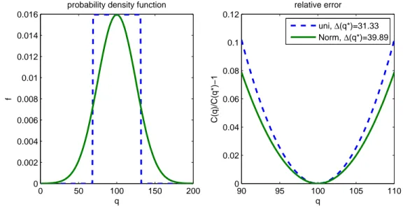
Figure 2-2: Probability density function and cost function (b = 5, h = 5) for a uniform and normal distribution. 0 50 100 150 200 0 0.002 0.004 0.006 0.008 0.01 0.012 0.014 0.016

probability density function

q f 90 95 100 105 110 0 0.02 0.04 0.06 0.08 0.1 0.12 q C(q)/C(q*)−1 relative error uni, ∆(q*)=31.33 Norm, ∆(q*)=39.89

distribution whose mass is concentrated around q∗ (i.e., has a small AMS) has a steeper cost function C around q∗. This is illustrated in Figure 2-2. The left plot shows the pdf of a Normal and a uniform distribution. The right plot shows the relative error (as a function of

q) when b = h = 5 and the optimal order quantity is 100 units for both distributions. The

uniform distribution, which has a smaller AMS, has a steeper error function. The decision of ordering 110 units has a larger relative error under the uniform distribution. On the other hand, the size of the conﬁdence interval for the quantile estimator of q∗ is inversely proportional to f (q∗) (Asmussen & Glynn, 2007). Thus, if f (q∗) is large, less samples are needed for the quantity ˜Qα_N to be close (in absolute terms) to q∗. In many distributions the absolute mean spread ∆(q∗) and the density value f (q∗) exhibit an inverse relationship. Therefore, a large weighted mean spread ∆(q∗)f (q∗) corresponds to a distribution for which this inverse relationship is balanced.

Recall the empirical experiment in§2.3 that produced Table 2.1. The experiment drew 1000 random samples, each with a sample size of N = 100, from a particular distribution. For each of these 1000 sets, the SAA solution was computed and its relative error is noted. (For these experiments, we simply take the _b+hb sample quantile and ignore the bias term. Biasing the SAA solution does not change the insights.) The empirical conﬁdence level is the fraction of the 1000 sets that achieve a relative error less than a target ϵ. Now, we can calculate the sample size predicted by Theorem 2.4.1 to match the empirical conﬁdence level for a target ϵ. The results are reported in Table 2.1 under the rows labeled Nf. Recall

that the empirical conﬁdence is generated from an actual sample size N = 100. We compare this with Nf and the sample size NLRS predicted by the LRS analysis (Theorem 2.3.1). We

ﬁnd that the sample size predicted by Theorem 2.4.1 using our new analysis are empirically signiﬁcantly smaller. NLRStypically has an order of magnitude between 100,000 to 1 million

(30)

Table 2.2: Regression analysis of ϵ = CNk b b+h = 0.8 b b+h = 0.9 b b+h = 0.95 k C R2 k C R2 k C R2 Uniform (A = 0, B = 100) -0.992 2.620 0.994 -1.002 2.807 0.992 -1.051 3.903 0.998 Normal (µ = 100, σ = 50) -1.016 3.155 0.994 -1.026 4.729 0.994 -0.97 5.131 0.994 Exponential (µ = 100) -0.983 3.066 0.995 -0.979 4.556 0.991 -1.02 9.712 0.998 Lognormal (µ = 1, σ = 1.805) -0.994 1.933 0.994 -1.014 4.384 0.995 -0.948 5.731 0.997 Pareto (xm= 1, α = 1.5) -1.021 2.977 0.997 -0.999 4.73 0.991 -0.984 7.85 0.992

samples, whereas Nf is typically between 100 to 1,000 samples.

2.4.1 Tightness of distribution-dependent bound

In what follows, we demonstrate through regression analysis that the new probability bound (Theorem 2.4.1) is indeed tight ; that is, it explains precisely how different factors influence the accuracy of the SAA procedure. First, we verify that it explains how the sample size influences the errors. We estimated empirically the error–sample size relationship by es-timating parameters C, k in the equation ϵ = CNk _{through regression. We fix a 90%}

conﬁdence level and cost parameters h = 1 and b. The number of samples N is varied from {100, 200, . . . , 1000}. For each N, a total of 1000 independent sets of N indepen-dent samples are drawn from a distribution. The SAA solutions {ˆq_N1, . . . , ˆq_N1000} are

cal-culated, and the resulting errors are labeled {ϵ1_N, . . . , ϵ1000_N } where ϵk_N = C(ˆq

k

N)−C(q∗)

C(q∗) . The 90% quantile of the errors is denoted by ϵN. We perform the regression using the data

{(100, ϵ100), (200, ϵ200), . . . , (1000, ϵ1000)}. Table 2.2 shows the estimated parameters as well as the R2 value. The probability bound of Theorem 2.4.1 explains a tight relationship if k is observed to be close to -1. From Table 2.2, all estimates for k are close to -1, and the estimated power function is almost a perfect ﬁt to the data (since R2 _{is close to 1).}

From Theorem 2.4.1, we can infer that the accuracy of the SAA procedure is only distribution-dependent through the weighted mean spread. We verify this by estimating the relationship ϵ = C{∆(q∗)f (q∗)}k through regression. We fix a 90% confidence level and a sample size N . We consider a pool of ten distributions, i.e., the five distributions in Table 2.2 each under two values of the newsvendor quantile, 0.9 and 0.95. Let ωi be the weighted

mean spread of distribution i. A total of 1000 independent sets of N independent samples are drawn from distribution i. We denote by ϵi the 90% quantile of the errors of the 1000

SAA solutions. We perform the regression using the data {(ω1, ϵ1), (ω2, ϵ2), . . . , (ω10, ϵ10)}. The results of the regression are reported in Table 2.3 for diﬀerent values of N . If k is close to -1, then Theorem 2.4.1 precisely explains the relationship between the error and weighted mean spread. From Table 2.3, we observe that all estimates for k are close to -1, and the R2 value is close to 1 signifying that the estimates are a close ﬁt to the data.

To conclude this section, we note that the probabilistic bound of Theorem 2.4.1 depends on the distribution only through the WMS ∆(q∗)f (q∗). However, computing it still requires

(31)

Table 2.3: Regression analysis of ϵ = C{∆(q∗)f (q∗)}k

N k C R2

100 -0.843 0.0166 0.928

300 -0.939 0.0048 0.990

500 -0.947 0.0029 0.993

knowledge of the speciﬁc underlying distribution. In the following section, we shall develop a new optimization framework to get a lower bound on the WMS for a family of distributions. This in turn leads to a uniform probability bound for that family. In particular, we obtain a uniform nonparametric probability bound for all log-concave distributions L.

2.5 Optimization-Driven Bound on WMS

In this section, we assume that the demand distribution f is such that it belongs toF, where F is a speciﬁed family of distributions. Suppose v∗ _{is a lower bound on the weighted mean}

spread ∆(q∗)f (q∗) of any distribution in F. Suppose we choose to bias ˜Qα

N, as deﬁned in

(2.8), by the factor α =√2ϵbhv∗+ O(ϵ). With minor changes to the proof of Theorem 2.4.1, we can show that C( ˜Qα_N)≤ (1 + ϵ)C(q∗) with probability at least 1− 2U∗(ϵ), where

U∗(ϵ)∼ exp (

−1

4N ϵv

∗)_{, as ϵ}_{→ 0.}

Note that both the bias factor and this new bound does not depend on speciﬁc parameters of the distribution beyond v∗. That is, unlike the bound in Theorem 2.4.1 which depends on the weighted mean spread, this bound is independent of any distribution parameters.

Next, we will use an optimization framework to ﬁnd a lower bound v∗ for a family of distributions F. This is accomplished by the following optimization problem:

inf f,q∗ ∆(q ∗_{)f (q}∗₎ s.t. f ∈ F, ∫ q∗ −∞f (s)ds = b b + h. (2.10)

Note that q∗ is a decision variable, but because of the second constraint, it is forced to take the value of the _b+hb quantile. Hence, (2.10) ﬁnds a distribution in F with the smallest WMS at the _b+hb quantile. Solving (2.10) or ﬁnding a lower bound v∗ on its optimal value provides a probability bound for the relative regret of ˜Qα_N over all demand distributions that belong to F.

In what follows, we will restrict our attention to the family of log-concave distributions L, which includes many of the distributions commonly used in inventory theory (Zipkin, 2000). We shall show that if F = L, then (2.10) can be solved in closed form. Moreover, the resulting probability bound on the relative regret incurred by the SAA solution is signiﬁcantly tighter than the LRS bound (2.5).

(32)

Deﬁnition 2.5.1 (Log-Concave Distribution). A distribution f with supportX is

log-concave if log f is log-concave inX .

It is known that the Normal distribution, the uniform distribution, the logistic distri-bution, the extreme-value distridistri-bution, the chi-square distridistri-bution, the chi distridistri-bution, the

exponential distribution, and the Laplace distribution are all log-concave for any respective

parameter values. Some families have log-concave density functions for some parameter regimes and not for others. Such families include the gamma distribution, the Weibull distribution, the beta distribution and the power function distribution. Note that L is not characterized through any parameterization (i.e, it does not depend on distributional parameters such as moments that need to be estimated), but rather describes properties satisﬁed by many common distributions.

Log-concave distributions are necessarily unimodal (Chandra & Roy, 2001). Any dis-tribution in this class must also have monotonic failure rate and reversed hazard rate (see Deﬁnition 2.5.2 below).

Deﬁnition 2.5.2 (Failure Rate and Reversed Hazard Rate). The failure rate is

defined as ₁_−Ff . The reversed hazard rate is defined as _Ff.

Log-concave distributions have both an increasing failure rate (IFR) and decreasing

reversed hazard rate (DRHR). Intuitively, this implies that the distribution falls oﬀ quickly

from its mode.

When we introduced our new analysis in §4, we made the technical assumption that

f is continuous everywhere. In fact, if f is log-concave, then it can have at most one

jump discontinuity, and the jump can only occur at the left end-point of its support (Sen-gupta & Nanda, 1997). Therefore, assuming that the demand distribution is log-concave automatically implies that this continuity assumption is also satisﬁed.

2.5.1 Probability bound for log-concave distributions

To solve (2.10) for log-concave distributions, we first solve a constrained version of (2.10). Specifically, for some γ0 > 0 and γ1, fix the value of q∗ and add the constraints f (q∗) = γ0 and γ1 ∈ ∂ log f(q∗), where ∂ log f (q∗) is the set of all subgradients of log f at q∗. The following optimization problem is obtained:

min f b + h h ∫ _∞ q∗ sf (s)ds−b + h b ∫ q∗ −∞sf (s)(ds) s.t. f ∈ L, ∫ q∗ −∞f (s)ds = b b + h, f (q∗) = γ0, γ1∈ ∂ log f(q∗). (2.11)

Note that since the density value f (q∗) is ﬁxed, the objective of the constrained problem reduces to minimizing the absolute mean spread ∆(q∗). The following lemma provides