Scale invariance of daily runoff time series in agricultural watersheds

HAL Id: hal-00304818

https://hal.archives-ouvertes.fr/hal-00304818

Submitted on 14 Feb 2006

HAL is a multi-disciplinary open access

archive for the deposit and dissemination of

sci-entific research documents, whether they are

pub-lished or not. The documents may come from

teaching and research institutions in France or

abroad, or from public or private research centers.

L’archive ouverte pluridisciplinaire HAL, est

destinée au dépôt et à la diffusion de documents

scientifiques de niveau recherche, publiés ou non,

émanant des établissements d’enseignement et de

recherche français ou étrangers, des laboratoires

publics ou privés.

agricultural watersheds

Xin Zhou, N. Persaud, H. Wang

To cite this version:

Xin Zhou, N. Persaud, H. Wang. Scale invariance of daily runoff time series in agricultural watersheds.

Hydrology and Earth System Sciences Discussions, European Geosciences Union, 2006, 10 (1),

pp.79-91. �hal-00304818�

www.copernicus.org/EGU/hess/hess/10/79/ SRef-ID: 1607-7938/hess/2006-10-79 European Geosciences Union

Earth System

Sciences

Scale invariance of daily runoff time series in agricultural

watersheds

X. Zhou1, N. Persaud2, and H. Wang3

1_{Department of Crop and Soil Sciences, The Pennsylvania State University, University Park, PA 16802, USA}

2_{Department of Crop and Soil Environmental Sciences, Virginia Polytechnic Institute and State University, Blacksburg, VA}

24061, USA

3_{Soil and Water Science Department, University of Florida, Gainesville, FL 32601, USA}

Received: 1 August 2005 – Published in Hydrology and Earth System Sciences Discussions: 30 August 2005 Revised: 24 November 2005 – Accepted: 20 December 2005 – Published: 14 February 2006

Abstract. Fractal scaling behavior of long-term records of

daily runoff time series in 31 sub-watersheds covering a wide range of size were examined using the shifted box-counting method and Hurst rescaled range (R/S) analysis. These sub-watersheds were associated with four agricultural sub-watersheds of different climate and topography. The results showed that the records of daily runoff rate exhibited scale invariance over certain time scales. Two scaling ranges were identi-fied from the shifted box-counting plots with a break point at about 9∼12 months. Similar fractal dimensions were ob-tained for the sub-watersheds within each watershed, indi-cating that the runoff of these sub-watersheds have similar distribution of occurrence. The Hurst R/S analysis showed that the long-term memory was not present in runoff time se-ries. The presence of scaling is not certain for runoff time series in agricultural watersheds.

1 Introduction

Current public policies and legislative mandates are strongly committed to the long term sustainable development and use of the nation’s watersheds, in particular protecting the quan-tity and quality of associated runoff-generated surface wa-ter resources (USEPA, 1995). Hydrologists have developed many mathematical models for predicting runoff in water-sheds. The development of most of these models has been based on observations taken over relatively small spatial and temporal scales. Since watersheds vary in their size, topog-raphy, land use pattern, hydrogeology, and drainage network morphology, the usefulness of these models depend on how well they can be extrapolated across spatial and temporal scales. This scale transfer problem, meaning the description

Correspondence to: X. Zhou

(xzz2@psu.edu)

and prediction of characteristics and processes at a scale dif-ferent from the one at which observations and measurements are made, remains a pervasive problem in many areas of sci-ence and engineering including hydrological scisci-ences (Spos-ito, 1998). The National Research Council (1991) stated: “. . . the search for an invariance property across scales as a basic hidden order in hydrologic phenomena, to guide devel-opment of specific models and new efforts in measurements is one of the main themes of hydrologic science”. Sposito (1998) reiterated: “. . . whether processes in the natural world are dependent or independent of the scale at which they op-erate is one of the major issues in hydrologic sciences”.

Parameters in runoff hydrological models are usually de-termined from monitoring data. However, stream networks in many watersheds in the USA are not gauged (or are par-tially gauged) and have no flow records, or the flow record is often too short to obtain the required hydrological param-eters. It would be very useful to find possible analytical tools that would enable extrapolation of observations of runoff processes in gauged watersheds or portions thereof, to pre-dict such processes in larger portions of the same watershed or in non-gauged watersheds (Bloschl and Sivapalan, 1995). Runoff processes are the direct result of the interaction of the spatial and temporal distribution of precipitation and water-shed physical characteristics such as topography and geol-ogy. Therefore extrapolation between scales of observations and between watersheds would require identifying and quan-tifying the scaling behavior of temporal and spatial water-shed characteristics and processes. Such information could result in reducing the extent and degree of monitoring re-quired by legislative mandates and lead to significant savings in cost and time.

We posit that fractal concepts and approaches provide the wherewithal to resolve this issue. There is already a signifi-cant body of evidence indicating that hydrological scaling or scale invariance can be successfully applied in hydrological

modeling (Bloschl and Sivapalan, 1995; Rodriguez-Iturbe and Rinaldo, 1997). Studies have shown that the scale invari-ance property is not only a feature of geometrical watershed characteristics, but may also be an inherent characteristic of hydrological dynamic processes (Schertzer and Lovejoy, 1987; Rodriguez-Iturbe and Rinaldo, 1997). Other reports indicate that some hydrological processes (e.g., rainfall), are spatially scale dependent processes (Gupta and Waymire, 1987). Scale invariant properties would be particularly use-ful in agricultural watersheds with sparse gauge networks, or where time series of rainfall and runoff records are relatively short (Olsson et al., 1992). Different from geometric scal-ing in classical geometrical objects, statistical scale invari-ance has been found to be more general and useful in natural processes and phenomena, which lead to relationships con-necting statistical properties of the geometric feature and/or dynamic processes at different scales. Mathematically, statis-tical scale invariance manifests itself when the dependence of number of observations in the series greater than a specified value on the values themselves follows a power law. Sta-tistical scale invariance is especially useful in the hydrology context since hydrological processes are often characterized by some statistical properties.

Since the demonstration of the validity of fractal con-cepts to describe natural objects by Mandelbrot (1983), the generality of the fractal nature of watershed hydrological characteristics and processes appears to be more and more widely acknowledged. Early researches were mostly focused on time series of rainfall records (Lovejoy and Schertzer, 1985; Olsson et al., 1992, 1993; Gupta and Waymire, 1993; Menabde et al., 1997; Schmitt et al., 1998). These studies have indicated that rainfall might be characterized by some time and/or space parameters, which are valid over a range of time and space scales. Not surprisingly, the results of these early studies of rainfall series led naturally and logi-cally to speculation that similar fractal spatial and temporal scaling characteristics exist for other watershed hydrological processes such as runoff and stream flows. Some recent re-ports have indicated that this is the case for regional flood frequencies in large natural drainage networks (Radziejew-ski and Kundzewicz, 1997; Robinson and Sivapalan, 1997; Pandey et al., 1998). A power law relationship was observed to hold between mean annual peak discharge per unit area and drainage area (Robinson and Sivapalan, 1997). Gupta et al. (1996) argued that the hypothesis of self-similarity pre-sented a powerful unifying theoretical framework, which can bridge statistical theory of regional flood frequency and im-portant empirical features in watershed topographic, rainfall, and flood data sets. Radeziejewski and Kundzewicz (1997) studied and identified the scale invariance of the daily river flow of the river Warta in Poland. They also combined sev-eral normalized flow series and evaluated the impact of such combinations on the fractal dimension. More recently, the scaling properties of runoff in karstic watersheds were also investigated (Labat et al., 2002).

The objective of present study was to investigate scale in-variance behavior of daily runoff rate time series for four agricultural watersheds and their 31 sub-watersheds. The scaling properties were examined by the fractal dimension estimated using the shifted box-counting method and by Hurst exponents estimated using rescaled range (R/S) anal-ysis.

2 Data and methods

2.1 Runoff data

The database developed by the Hydrological and Remote Sensing Laboratory of the Agricultural Research Service of the US Department of Agriculture (USDA/ARS/HRSL) was the source of the hydrological data analyzed in this study. It consisted primarily of rainfall/runoff data from the ARS monitored experimental agricultural watersheds nationwide. These watersheds represent numerous land uses and agricul-tural practices and cover a diverse range of climatic condi-tions across the U.S. About 16 600 station years of rainfall and runoff were available in the database.

Four agricultural watersheds were selected from the database: (1) the Little River watershed, Southeast Water-shed Research Laboratory, Tifton, Georgia; (2) the Little Mill Creek watershed in the North Appalachian Experimental Wa-tershed, Coshocton, Ohio; (3) the Reynolds Creek waWa-tershed, Northwest Watershed Research Center, Boise, Idaho; and (4) the Sleepers River watershed, Danville, Vermont. Sev-eral factors were taken into account in selecting watersheds for investigation, including length and completeness of the records, watershed and sub-watershed sizes, and availability of other ancillary information. Some descriptions of these studied watersheds were listed in Table 1.

Each watershed selected contained a number of sub-watersheds and their properties are summarized in Table 2. A total of 31 sub-watersheds was analyzed. These sub-watersheds covered a wide range of sizes from 0.01 km2 (sub-watershed W-23 of the Reynolds Creek watershed) to 334 km2 (sub-watershed W-TB of the Little River water-shed). Surface runoff in these sub-watersheds was measured and recorded at various intervals, from a few minutes to sev-eral hours. In gensev-eral, more frequent measurements were made during rain days. The runoff records within each day were integrated to obtain daily runoff time series for further analysis.

2.2 Shifted box-counting analysis

The records of a runoff time series can be regarded as a bi-nary set of points, which is defined on some threshold value. Zero is generally used as a default threshold value, though other values >0 can be also used. In this case, only the observations with the value greater than the threshold are considered as points of the derived set. In this study, four

Table 1. Description of four studied watersheds.

Watershed Area Elevation Mean Drainage Land use precipitation density

(km2) (m) (mm) (km/km2)

Little River Watershed, GA 334 82–148 1140 2.3 Agriculture and forestry are dominant

Little Mill Creek Watershed, OH 19 248–393 1245 2.6 Forest (40%), Cropland (25%), and Pasture (20%) Reynolds Creek Watershed, ID 234 1101–2241 230 at lower elevation and 3.0 Livestock grazing with some

>1100 in higher regions irrigate fields along the creek Sleepers River Watershed, VT 111 206–784 1100 3.3 Typical northern hardwood forest with about one-third of the watershed in pasture land use for dairy farming

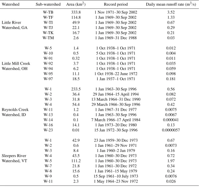
Table 2. Daily runoff records in agricultural watersheds and sub-watersheds studied.

Watershed Sub-watershed Area (km2) Record period Daily mean runoff rate (m3/s) W-TB 333.8 1 Nov 1971–30 Sep 2002 3.52

W-TF 114.8 1 Jan 1969–30 Sep 2002 1.33 Little River W-TI 49.9 1 Jan 1969–30 Sep 2002 0.67 Watershed, GA W-TJ 22.1 1 Jan 1969–30 Sep 2002 0.29 W-TK 16.7 1 Jan 1969–30 Sep 2002 0.21 W-TM 2.6 1 Jan 1969–31 Dec 1988 0.03 W-5 1.4 1 Oct 1938–1 Oct 1971 0.012 W-10 0.5 5 Oct 1938–1 Oct 1971 0.004 W-91 0.32 1 Oct 1938–1 Oct 1971 0.011 Little Mill Creek W-92 3.7 1 Oct 1938–1 Oct 1971 0.035 Watershed, OH W-94 6.2 1 Oct 1938–1 Oct 1971 0.059 W-95 11.1 1 Oct 1938–22 June 1972 0.098 W-97 18.5 1 Jan 1937–1 Oct 1971 0.181 W-1 233.5 1 Jan 1963–30 Sep 1996 0.56 W-2 36.4 29 Jan 1964–15 April 1994 0.082 W-3 31.8 13 March 1964–31 Dec 1990 0.072 W-4 54.4 29 March 1966–30 Sep 1996 0.42 Reynolds Creek W-11 1.2 1 Jan 1967–31 Dec 1977 0.0075 Watershed, ID W-13 0.4 1 Jan 1963–30 Sep 1996 0.0067 W-14 0.1 7 March 1966–17 April 1984 0.000041 W-16 14.1 1 Jan 1973–20 Dec 1980 0.13 W-23 0.01 15 Jan 1972–30 Sep 1996 0.0000057 W-1 42.9 23 Jan 1959–30 Dec 1973 0.67 W-2 0.6 1 Jan 1961–29 Nov 1971 0.0073 W-3 8.4 1 Jan 1960–2 Jan 1979 0.16 Sleepers River W-4 43.5 1 Jan 1960–30 Dec 1973 0.72 Watershed, VT W-5 111.2 1 Jan 1960–30 Dec 1973 1.97 W-7 21.8 1 Jan 1961–30 Dec 1972 0.34 W-8 15.6 1 Jan 1961–15 May 1979 0.24 W-9 0.5 15 Sep 1961–10 July 1973 0.0076 W-11 2.3 1 May 1964–23 Nov 1972 0.026

threshold levels of the runoff rate (0, 0.5 M, M, and 1.5 M, where M is the average daily runoff rate) were used to define the sets. The scaling property of the runoff data series was measured on the resulting sets by the shifted box-counting method, which is an improvement proposed by Radziejewski and Kundzewicz (1997) on the conventional box-counting method.

In this method, a uniform one-dimensional grid of box size ε was superimposed onto the time domain on which the series is defined. The number of non-overlapping grid segments (boxes) needed to cover the whole series to be analyzed was counted. Only those boxes that contained at least one element that was above the threshold value were counted. The grid position was then shifted in time different units, from 1 to ε–1. The number of boxes, N(ε), contain-ing elements of the set of interest for all possible shifts were counted, and finally the counts were averaged.

Different box sizes were used to cover the sets. The mini-mum box size (ε) used was one day, and then the size was doubled (i.e., 2, 4, 8, . . . ), until the maximum size (1/5 of the data length) was reached. For sufficiently small ε,

N(ε)∝(1/ε). The relationship of N(ε) versus ε was fitted to a

power law function:

N (ε) = C (1/ε)D (1) where C and D are constant values. The fractal dimension, (D), was calculated as:

D = lim

ε→0(log N (ε) − log c)/(log(1/ε)) (2)

In applying this method log N(ε) was plotted versus log (1/ε), and D was estimated from the graph as the slope of the straight line best fitted to the points.

2.3 Rescaled range (R/S) analysis

Hurst (1951) studied the 847-year record of the overflows of the Nile River, and found that successive observations in the series above or below the mean value tended to persist. He termed this tendency “long-term persistence” or “long-term memory”. Hurst’s subsequent investigations showed that this phenomenon was characteristic of the overflow, water stor-age, and stream flow of many other rivers. While other meth-ods have also been proposed (Montanari et al., 1997; Hu et al., 2001; Markovic and Koch, 2005), detecting such per-sistence phenomena in hydrological series is classically ob-tained by the adjusted rescaled range (R/S) analysis (Man-delbrot and Wallis, 1969; Peters, 1994; Zhou et al., 2005), This analysis involves a statistical rescaling of the original series over lag times of varying widths. The procedures of

R/Sanalysis used are described in detail as follows: Let X(t) be a time series of recorded runoff containing

N readings from t =1 to t =N . Let X∗(t )=Xt +1, . . . , Xt +n,

represent consecutive observation values within a subset of the record from t + 1 to time t+n. The lag time n denotes

the interval of the subset, and t denotes the starting point for the subset. The mean value, Xm, of the time series X∗(t )is

defined as: Xm=( i=t +n X i=t +1 Xi)/n (3)

The standard deviation of the subset from t+1 to time t +n,

Sn, is estimated as: Sn=n−1/2× v u u t t +n X r=t +1 (Xr−Xm)2 (4)

The rescaled range is calculated by first rescaling the subset data by subtracting the sample mean of X∗(t )as:

Zr =(Xr −Xm) r = t +1, ..., t + n (5)

And the cumulative time series, Y , is created by:

Yr+1=Zt +1 r = t +1 (6)

Yr =(Yr−1+Zr) r = t +2, ..., t + n (7)

The adjusted range, Rn, is the accumulative departure from

the mean, i.e. the maximum minus the minimum value of Yr:

Rn=max(Yt +1, ..., Yt +n) −min(Yt +1, ..., Yt +n) (8)

For the interval starting at time t , of width n, R and S are computed. This is repeated for each successive t, until t reaches N −n+1. The procedures are repeated for the next lag time n, until all selected lags have been tested. A general form of the relationship of R/S to n (Hurst, 1951):

(R/S)n=c × nH (9)

A log transformation of Eq. (9) gives

log(R/S) = H log n + log c (10)

Exponent H is estimated from the graph as the slope of the straight line best fitted to the points. The small lags only represent short-term memory, thus should not be used to es-timate H values (Taqqu et al., 1995). It should be noted that H>0.5 may be obtained from R/S method even when a long-term memory is not present in a time series (Taqqu et al., 1995; Montanari, 2003).

The empirically defined Hurst exponent is related to the theoretical fractal dimension D of the graph of a correspond-ing time series, as:

D =2 − H (11)

The scaling analysis on long-term persistence is influenced by the inherent deterministic component (trends and period-icities) of the time series, which is particular true for hy-drological or meteorological time series (Hu et al., 2001; Kallache et al., 2005). It has been suggested that the deter-ministic components should be separated from its stochastic

ε _(day) 0.1 1 10 100 1000 10000 N ( ε) 1e+0 1e+1 1e+2 1e+3 1e+4 1e+5 0 1.76 3.52 5.28 Threshold

Fig. 1. Log-log plots of number of boxes [N(ε)] versus box size (ε) for different threshold values (0, 1.76, 3.52, and 5.28 m3/s) using the shifted box counting method to analyze the runoff rate series for sub-watershed W-TB of the Litter River watershed in Tifton, Georgia. In all cases, r2was >0.99 for the straight lines fitted to the sections of the graph. Box sizes were exponentially doubled starting at ε=1 day.

components prior to drawing a conclusion on the time se-ries scaling structure (Klemes, 1974; Montanari et al., 1997; Radziejewski and Kundzewicz, 1997; Markovic and Koch, 2005). Many approaches have been proposed to distinguish the deterministic components and long-range components (Taqqu et al., 1995; Montanari et al., 1999; Maraun et al., 2004).

The daily runoff time series were transformed as follows to obtain a process without seasonality (time series with zero mean and unit standard deviation): (1) logarithms of data series, (2) subtracted seasonal mean values of the time se-ries, and (3) divided by seasonal standard deviations of the time series. The shifted box-counting method and R/S anal-ysis were also applied on these transformed time series to investigate the seasonal effects on scaling characterization in agricultural watersheds.

3 Results and discussion

3.1 Estimated fractal dimension

An example of the shifted box-counting graph log N(ε) ver-sus log ε for the runoff time series in sub-watershed W-TB of the Little River watershed is displayed in Fig. 1. The mean daily runoff rate in this example was 3.52 m3s−1 (Ta-ble 2). Since log N(ε) versus log ε was plotted instead of log

N(ε) versus log (1/ε), the value of the negative slope

repre-sents the estimated fractal dimension of the sets. It should be noted that the fractal dimensions were estimated for some bi-nary sets derived from the runoff series based on the chosen threshold values, not the runoff series itself. The box sizes

ε _(day) 0.1 1 10 100 1000 10000 N ( ε) 1e+0 1e+1 1e+2 1e+3 1e+4 1e+5 0 1.76 3.52 5.28 Threshold

Fig. 2. Shifted box counting graph as in Fig. 1 but with one day in-crement of box size (ε) for sub-watershed W-TB of the Litter River watershed in Tifton, Georgia. The break point of the slope occurs at approximately ε=365 days.

(time scales) were between one day and 1/5 of the length of the records. If the runoff time series possessed a scale-invariance property, a straight line could be fitted to the box-counting graph or part of it, according to the Eq. (2). Figure 1 shows that for each threshold, two distinct scaling ranges are apparent, each of which can be fitted with a straight-line sec-tion by least square regression, instead of a single linear re-lationship over the entire range of time scales.

The existence of linear relationship over certain time scales indicates that there is a scale invariant distribution of runoff in time, which is valid within the defined linear scaling range. By using fractal concepts, temporal scale invariance of runoff might be characterized by a single parameter, frac-tal dimension (D). Since two D values were obtained from the box-counting analysis for the time series in Fig. 1 over the time period under consideration, it implies that its scal-ing properties vary with the time scales.

Likewise, the runoff time series of other five sub-watersheds in the Little River watershed as well as all the sub-watersheds in the other watersheds studied (Little Mill Creek watershed, Reynolds Creek watershed, and Sleepers River watershed) all displayed two scaling ranges for each threshold in their box-counting graphs. The break point [in-tersection of the two straight line sections in the log N(ε) ver-sus log ε plots] for all thresholds corresponded to the same box size, which indicates the same scaling ranges are valid no matter what runoff intensity threshold was used to define the set.

To further precisely locate the break point, the box-counting technique was applied with one-day increment of box size (Fig. 2) instead of the exponential doubling incre-ments used for Fig. 1. In Fig. 2, the break point was found to correspond to a box size of approximately 365 days. This

Table 3. Fractal dimensions (D) of daily runoff rate for six sub-watersheds of the Little River watershed in Tifton, Georgia. Fractal dimensions correspond to four threshold levels of the original runoff rate and five thresholds of the transformed series.

Original runoff series Transformed runoff series Sub-watershed Threshold (m3s−1) D r2 Threshold D r2

0 0.96 0.999 −1 0.95 0.999 1.76 0.81 0.998 −0.5 0.93 0.999 W-TB 3.52 0.76 0.997 0 0.89 0.999 5.28 0.71 0.994 0.5 0.81 0.999 1 0.65 0.999 0 0.94 0.999 −1 0.96 0.999 0.66 0.83 0.998 −0.5 0.92 0.999 W-TF 1.33 0.77 0.995 0 0.89 0.999 2.00 0.71 0.991 0.5 0.81 0.999 1 0.64 0.999 0 0.93 0.999 −1 0.96 0.999 0.33 0.83 0.997 −0.5 0.91 0.999 W-TI 0.67 0.77 0.995 0 0.89 0.999 1.00 0.70 0.991 0.5 0.81 0.999 1 0.65 0.999 0 0.92 0.999 −1 0.98 0.999 0.15 0.81 0.996 −0.5 0.89 0.999 W-TJ 0.30 0.74 0.994 0 0.88 0.999 0.45 0.68 0.990 0.5 0.81 0.999 1 0.68 0.997 0 0.92 0.999 −1 0.97 0.999 0.10 0.84 0.997 −0.5 0.92 0.999 W-TK 0.20 0.79 0.996 0 0.89 0.999 0.30 0.73 0.994 0.5 0.81 0.999 1 0.66 0.999 0 0.96 0.999 −1 0.96 0.999 0.015 0.83 0.998 −0.5 0.95 0.999 W-TM 0.030 0.76 0.996 0 0.90 0.999 0.045 0.69 0.991 0.5 0.80 0.999 1 0.63 0.993

may be explained by the obvious annual cycle of all the runoff time series. It has been suggested that the seasonal cycles should be removed from the original data prior to drawing conclusions on time series scaling structure (Mon-tanari et al., 1997; Markovic and Koch, 2005). The shifted box-counting method was also used to estimate the fractal dimensions of the deseasonalized time series, which have zero mean and unity standard deviation. Five threshold val-ues (−1, −0.5, 0, 0.5, and 1) were used to derive the binary sets. The results showed that two scaling ranges were also observed for the deseasonalized runoff series and the break point again occurred at about 9∼12 months (Fig. 3), although fractal dimensions changed in scaling range of small box sizes (Table 3). For example, at the threshold of data mean

(3.52 m3s−1for original time series, and 0 for transformed time series), D increased from 0.76 (original) to 0.89 (desea-sonalized). The fractal dimensions in scaling range of large box sizes were approximately equal to 1.0, and not sensitive to threshold values.

The fact that two scaling ranges were apparent would in-dicate that the scaling characteristics of the short-term pro-cess (<1 year) and long-term propro-cess (>1 year) of water-shed runoff were different. Breakpoints in scaling ranges for watershed runoff were also found in other studies us-ing the shifted box-countus-ing analysis. In their investigation of daily flows of the river Warta in Poland, Radziejewski and Kundzewicz (1997) reported a distinct break point in the scaling ranges at approximately 2–4 years. They also

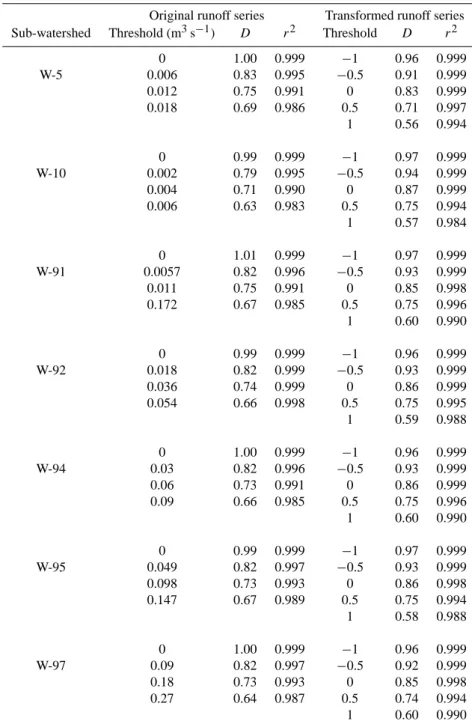
Table 4. Fractal dimensions (D) of daily runoff rate for seven sub-watersheds of the Little Mill Creek watershed in Coshocton, Ohio. Fractal dimensions correspond to four threshold levels of the original runoff rate and five thresholds of the transformed series.

Original runoff series Transformed runoff series Sub-watershed Threshold (m3s−1) D r2 Threshold D r2

0 1.00 0.999 −1 0.96 0.999 W-5 0.006 0.83 0.995 −0.5 0.91 0.999 0.012 0.75 0.991 0 0.83 0.999 0.018 0.69 0.986 0.5 0.71 0.997 1 0.56 0.994 0 0.99 0.999 −1 0.97 0.999 W-10 0.002 0.79 0.995 −0.5 0.94 0.999 0.004 0.71 0.990 0 0.87 0.999 0.006 0.63 0.983 0.5 0.75 0.994 1 0.57 0.984 0 1.01 0.999 −1 0.97 0.999 W-91 0.0057 0.82 0.996 −0.5 0.93 0.999 0.011 0.75 0.991 0 0.85 0.998 0.172 0.67 0.985 0.5 0.75 0.996 1 0.60 0.990 0 0.99 0.999 −1 0.96 0.999 W-92 0.018 0.82 0.999 −0.5 0.93 0.999 0.036 0.74 0.999 0 0.86 0.999 0.054 0.66 0.998 0.5 0.75 0.995 1 0.59 0.988 0 1.00 0.999 −1 0.96 0.999 W-94 0.03 0.82 0.996 −0.5 0.93 0.999 0.06 0.73 0.991 0 0.86 0.999 0.09 0.66 0.985 0.5 0.75 0.996 1 0.60 0.990 0 0.99 0.999 −1 0.97 0.999 W-95 0.049 0.82 0.997 −0.5 0.93 0.999 0.098 0.73 0.993 0 0.86 0.998 0.147 0.67 0.989 0.5 0.75 0.994 1 0.58 0.988 0 1.00 0.999 −1 0.96 0.999 W-97 0.09 0.82 0.997 −0.5 0.92 0.999 0.18 0.73 0.993 0 0.85 0.998 0.27 0.64 0.987 0.5 0.74 0.994 1 0.60 0.990

detected another less distinct break point located at 10–15 days.

Estimated fractal dimensions in the scaling region less than 1 year are summarized in Table 3 through 6 for each of the four watersheds. If we term the scaling range of box size less than 1 year as range 1, and as 2 otherwise, the fractal dimension in range 1 decreases as the threshold in-creases for both the original and deseasonalized series. In

range 1, for example, D decreases from 0.96 at 0 m3s−1 to 0.71 at 5.28 m3s−1 for the original runoff time series of sub-watershed W-TB (Table 3). However, the fractal dimen-sions at range 2 show almost no change for various thresh-olds with D=1.0 (Figs. 1 and 3). The dependence of the es-timated fractal dimension on the defined threshold value was also observed in previous studies (Olsson et al., 1992, 1993; Radziejewski and Kundzewicz, 1997). In all of these studies,

Table 5. Fractal dimensions (D) of daily runoff rate for nine sub-watersheds of the Reynolds Creek watershed in Boise, Idaho. Fractal dimensions correspond to four threshold levels of the original runoff rate and five thresholds of the transformed series.

Original runoff series Transformed runoff series Sub-watershed Threshold (m3s−1) D r2 Threshold D r2

0 1.00 0.999 −1 0.97 0.999 W-1 0.28 0.82 0.997 −0.5 0.93 0.999 0.56 0.77 0.996 0 0.88 0.999 0.84 0.72 0.994 0.5 0.81 0.999 1 0.67 0.999 0 1.00 0.999 −1 0.98 0.999 W-2 0.041 0.85 0.998 −0.5 0.95 0.999 0.082 0.76 0.996 0 0.89 0.999 0.5 0.79 0.999 0.123 0.70 0.994 1 0.63 0.997 0 1.00 0.999 −1 0.97 0.999 W-3 0.036 0.81 0.998 −0.5 0.93 0.999 0.072 0.74 0.996 0 0.88 0.999 0.108 0.68 0.995 0.5 0.80 0.999 1 0.63 0.999 0 1.00 0.999 −1 0.98 0.999 W-4 0.21 0.82 0.997 −0.5 0.94 0.999 0.42 0.75 0.996 0 0.89 0.999 0.63 0.72 0.994 0.5 0.81 0.998 1 0.65 0.995 0 0.98 0.999 −1 0.98 0.999 W-11 0.0038 0.84 0.998 −0.5 0.92 0.999 0.0075 0.77 0.998 0 0.88 0.999 0.0113 0.72 0.997 0.5 0.79 0.998 1 0.64 0.999 0 1.00 0.999 −1 0.97 0.999 W-13 0.0034 0.76 0.993 −0.5 0.93 0.999 0.0067 0.80 0.990 0 0.86 0.999 0.0100 0.79 0.989 0.5 0.75 0.999 1 0.60 0.997 0 0.72 0.994 −1 1.00 0.999 W-14 0.00002 0.67 0.995 −0.5 0.98 0.999 0.00004 0.65 0.995 0 0.72 0.990 0.00006 0.63 0.993 0.5 0.64 0.999 1 0.56 0.999 0 1.00 0.999 −1 0.97 0.999 W-16 0.065 0.84 0.999 −0.5 0.94 0.999 0.130 0.77 0.998 0 0.90 0.999 0.195 0.74 0.996 0.5 0.78 0.997 1 0.62 0.997 0 0.41 0.976 −1 1.0 0.999 W-23 0.00000028 0.41 0.976 −0.5 1.0 0.999 0.00000057 0.41 0.976 0 0.92 0.998 0.00000084 0.41 0.977 0.5 0.88 0.999 1 0.43 0.996

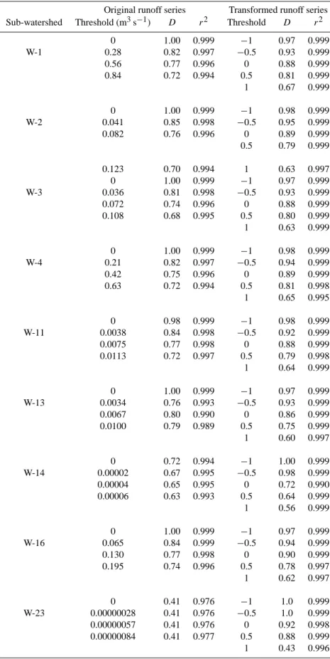
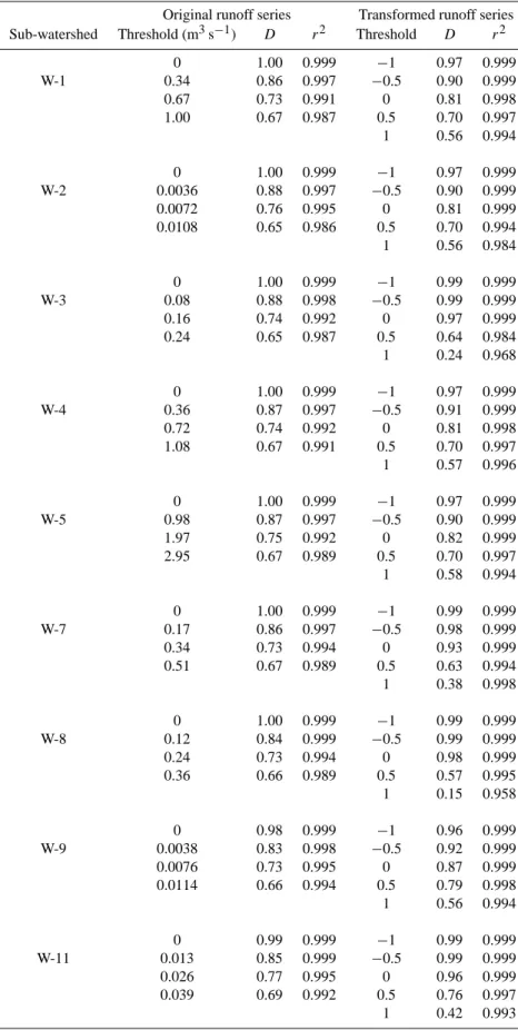
Table 6. Fractal dimensions (D) of daily runoff rate for nine sub-watersheds of the Sleepers Creek watershed in Vermont. Fractal dimensions correspond to four threshold levels of the original runoff rate and five thresholds of the transformed series.

Original runoff series Transformed runoff series Sub-watershed Threshold (m3s−1) D r2 Threshold D r2

0 1.00 0.999 −1 0.97 0.999 W-1 0.34 0.86 0.997 −0.5 0.90 0.999 0.67 0.73 0.991 0 0.81 0.998 1.00 0.67 0.987 0.5 0.70 0.997 1 0.56 0.994 0 1.00 0.999 −1 0.97 0.999 W-2 0.0036 0.88 0.997 −0.5 0.90 0.999 0.0072 0.76 0.995 0 0.81 0.999 0.0108 0.65 0.986 0.5 0.70 0.994 1 0.56 0.984 0 1.00 0.999 −1 0.99 0.999 W-3 0.08 0.88 0.998 −0.5 0.99 0.999 0.16 0.74 0.992 0 0.97 0.999 0.24 0.65 0.987 0.5 0.64 0.984 1 0.24 0.968 0 1.00 0.999 −1 0.97 0.999 W-4 0.36 0.87 0.997 −0.5 0.91 0.999 0.72 0.74 0.992 0 0.81 0.998 1.08 0.67 0.991 0.5 0.70 0.997 1 0.57 0.996 0 1.00 0.999 −1 0.97 0.999 W-5 0.98 0.87 0.997 −0.5 0.90 0.999 1.97 0.75 0.992 0 0.82 0.999 2.95 0.67 0.989 0.5 0.70 0.997 1 0.58 0.994 0 1.00 0.999 −1 0.99 0.999 W-7 0.17 0.86 0.997 −0.5 0.98 0.999 0.34 0.73 0.994 0 0.93 0.999 0.51 0.67 0.989 0.5 0.63 0.994 1 0.38 0.998 0 1.00 0.999 −1 0.99 0.999 W-8 0.12 0.84 0.999 −0.5 0.99 0.999 0.24 0.73 0.994 0 0.98 0.999 0.36 0.66 0.989 0.5 0.57 0.995 1 0.15 0.958 0 0.98 0.999 −1 0.96 0.999 W-9 0.0038 0.83 0.998 −0.5 0.92 0.999 0.0076 0.73 0.995 0 0.87 0.999 0.0114 0.66 0.994 0.5 0.79 0.998 1 0.56 0.994 0 0.99 0.999 −1 0.99 0.999 W-11 0.013 0.85 0.999 −0.5 0.99 0.999 0.026 0.77 0.995 0 0.96 0.999 0.039 0.69 0.992 0.5 0.76 0.997 1 0.42 0.993

ε (day) 1 10 100 1000 10000 N ( ε) 1 10 100 1000 10000 -1 -0.5 0 0.5 1 Threshold

Fig. 3. Log-log plots of number of boxes [N(ε)] versus box size (ε) for different threshold values (−1, −0.5, 0, 0.5, 1) using the shifted box counting method to analyze the deseasonalized runoff rate series for sub-watershed W-TB of the Litter River watershed in Tifton, Georgia.

a fractal dimension of 1.0 was obtained when the time scale exceeded a certain value, which was about 365 days in this study.

For the original runoff series in this study, for the 0 m3s−1 threshold, D appropriates or equals to 1.0 for all the runoff series (Tables 3∼6). This might be because the observations of daily runoff intensity are nearly all greater than 0, there-fore, the generated set is almost continuous with few gaps (no runoff) between them. As a result, a smaller dimension was obtained from the box-counting plot. In scaling range 2 where the box sizes are greater than one year the fractal di-mension is equal to 1.0 at all the threshold levels (Fig. 1). This might be because there would always have at least one day of a year that the runoff rate exceeded the threshold value. The regression coefficients of regression lines in the log N(ε) versus log ε plots were high for all the runoff time series with values greater than or close to 0.990, which indi-cates a strong linear relation. These consistently high values are considered requisite to provide confidence in any infer-ence that the runoff series under investigation demonstrate scale invariant characteristics.

Table 3 indicates that the fractal dimensions for all the 6 sub-watersheds of the Little River watershed at each level of the threshold were almost the same, although the con-tribution areas of these sub-watersheds are quite different (2.6∼333.8 km2 for sub-watersheds of the Little River wa-tershed as listed in Table 2). The sub-wawa-tersheds of the Lit-tle River watershed as an example, the D-value of original runoff series ranged from 0.92 to 0.96 for threshold level 1, 0.81 to 0.83 for level 2, 0.74 to 0.79 for level 3, and 0.68 to 0.71 for level 4 (Table 3). The same pattern was found in all the other three watersheds (Tables 3 through 5).

The results presented in Tables 3 through 6, and the log

N(ε) versus log ε box-counting plots for the runoff time

se-ries were quite consistent across the sub-watersheds of the four watersheds. With the exception of the two smallest sub-watersheds (W-14 and W-23 of the Reynolds Creek wa-tershed), the same fractal dimension (estimated using the shifted box-counting method) was obtained for the runoff se-ries at each threshold level although these watersheds varied markedly in climate, topography, and size (Table 2). For ex-ample, for a given threshold level, say level 2, the fractal di-mension is about 0.85 for practically all the runoff time series in four watersheds (Tables 2 to 5). In other words, runoff time series in these watersheds and their sub-watersheds have sim-ilar distribution of occurrence of runoff, and exhibit the same pattern of scaling, although they have different climates, ge-ography, soil type, land management, etc.

It should be pointed out that the threshold values used to define the binary sets from the original runoff series were different for time series because the mean daily runoff rates of the sub-watersheds were different (Table 2). Selecting threshold values based on mean daily runoff rates allows comparison of the fractal dimensions estimated from differ-ent runoff time series. The results indicated that although the daily runoff rates were different by orders of magnitude (Table 2), the occurrence of runoff had the same distribution. The transformed series have zero mean and unity standard deviation, therefore the same threshold values (−1, −0.5, 0, 0.5 and 1) were used for all the time series.

At threshold level 4, the fractal dimensions of runoff time series for the Little Mill Creek and Sleepers River water-sheds were slightly less than that for the Little River and Reynolds Creek watersheds. A lower dimension means that more points are clustered in groups over time scales. Thus it indicated that high runoff occurrences are more clustered in the Little Mill Creek and Sleepers River watersheds than the other two watersheds.

As discussed above, the occurrence of runoff in agricul-tural sub-watersheds of various sizes had similar distribu-tion, making it possible to extrapolate runoff behavior over a fairly large range of spatial scales within a watershed. How-ever, this scaling property may not be valid when the sub-watersheds are small. The box dimension of the runoff series for the two smallest sub-watersheds (W-14=0.01 km2and W-23=0.1 km2)of the Reynolds Creek watershed, were much lower and did not change at different threshold levels (Ta-ble 5). It indicated that the distribution of runoff occurrence in extremely small sub-watersheds might be different from larger watersheds, and extrapolation might not be feasible at relatively small scales. One possible explanation might be that the total volume of surface runoff from a very small sub-watershed is limited, and measured runoff tends to be almost zero at most of the time depending on the sensitivity and res-olution of the measuring instruments. On the other hand, for the runoff series investigated in this study, no upper restric-tion of sub-watershed size in scaling was detected.

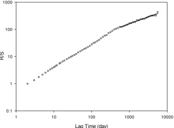
Lag Time (day) 1 10 100 1000 10000 R /S 0.1 1 10 100 1000

Fig. 4. Hurst rescaled range analysis plot for daily runoff time se-ries of sub-watershed W-TB of the Little River watershed in Tifton, Georgia. A straight line was fitted to the large lags.

3.2 Estimated Hurst exponent

The Hurst exponent (H ) as a useful parameter to describe long-term persistence of observations in hydrological time series was initially applied in an empirical manner to water reservoir design (Hurst, 1951). It was later established that the Hurst exponent could be theoretically related to the frac-tal dimension for idealized time series that can be modeled as fractional Brownian motions. Figure 4 shows an example of the rescaled range plot used to obtain the Hurst exponent of the original runoff time series for sub-watershed W-TB in the Little River watershed. In the plot, two distinct scaling ranges are clearly displayed. H values should be estimated from the large lags in R/S plots since the small lags only represent short-term memory (Taqqu and Teveroski, 1995; Montanari et al., 2003). A straight line was fitted to the scal-ing range by least square regression. The H values of each runoff time series are presented in Table 7.

Generally, H values of most runoff time series are around 0.50 (Table 7) indicating a random process (Mandelbrot and Wallis, 1969). Little River Watershed as an example, H val-ues range from 0.46 to 0.51 for sub-watersheds. For the Sleepers River sub-watershed group, the H values are much less than 0.50 (Table 7). A Hurst exponent of H <0.5 char-acterizes an unstable phenomenon, and it is unusual in nat-ural hydrological system (Beran, 1994). Most of river flows possess an H value around 0.7 (Hurst, 1951). The seasonal cycle was removed from the original time series for R/S anal-ysis. Figure 5 shows the R/S plot for W-TB sub-watershed of the Little River watershed after deseasonalization. The

Hvalues surprisingly increase for deseasonalized runoff se-ries compared to H values of the original sese-ries (Fig. 4 and Table 7). Different from the original time series, the de-seasonalized runoff time series have H values much greater

Lag Time (day)

1 10 100 1000 10000 R /S 0.1 1 10 100 1000

Fig. 5. Hurst rescaled range analysis plot for deseasonalized daily runoff time series of sub-watershed W-TB of the Little River wa-tershed in Tifton, Georgia. A straight line was fitted to the large lags.

than 0.5 at large lags with typical value around 0.7, which indicates a long-term memory (Table 7). H values in the Reynolds Creek watershed and Sleepers River watershed are greater than those in the Little River watershed and Little Mill Creek watershed (Table 7). This is unexpected since long-term memory will not be removed by superimposing a periodic component. A satisfactory explanation of such un-usual behavior in this study is not found. It should be noted that the runoff time series of these agricultural watersheds are quite short, especially for the Sleepers River watershed and Reynolds Creek watershed (Table 2), therefore the esti-mation of long-term memory based on R/S plots might not be reliable.

4 Conclusions

The scaling property of daily runoff for 31 sub-watersheds covering a wide range of sizes in four agricultural watersheds of different climate and topography was examined using the shifted box-counting method and Hurst rescaled range anal-ysis. The same analyses were also applied to the deseason-alized runoff time series. The results from fractal dimension estimation showed that long-term records of daily runoff rate exhibited scale invariance over certain time scales. Two scal-ing ranges were identified in the shifted box-countscal-ing plots with a break point at about 9∼12 months. The same frac-tal dimensions were obtained for the sub-watersheds within each watershed, indicating that the runoff of these sub-watersheds have similar distribution of occurrence and scal-ing behavior. However, the Hurst analysis showed that the daily runoff time series are lack of long-term memory, and therefore lack of scaling, although they showed short-term memory. The presence of scaling is not certain for runoff

Table 7. Hurst exponents (H ) of daily runoff time series estimated using the R/S analysis method.

Watershed Sub-watershed H H

(Original) (Deseasonalized)

W-TB 0.50 0.65

W-TF 0.49 0.71

Little River W-TI 0.48 0.68

Watershed, GA W-TJ 0.51 0.64 W-TK 0.51 0.66 W-TM 0.46 0.79 Average 0.49 0.69 W-5 0.52 0.72 W-10 0.51 0.65 W-91 0.46 0.72

Little Mill Creek W-92 0.46 0.70

Watershed, OH W-94 0.47 0.73 W-95 0.46 0.70 W-97 0.53 0.65 Average 0.49 0.70 W-1 0.60 0.86 W-2 0.54 0.91 W-3 0.60 0.94 W-4 0.59 0.92 Reynolds Creek W-11 0.53 0.91 Watershed, ID W-13 0.43 0.90 W-14 0.60 N/A W-16 0.27 0.95 W-23 0.37 N/A Average 0.50 0.91 W-1 0.45 0.66 W-2 0.30 0.79 W-3 0.41 0.85 Sleepers River W-4 0.32 0.70 Watershed, VT W-5 0.29 0.63 W-7 0.39 0.93 W-8 0.35 0.83 W-9 0.42 0.69 W-11 0.63 0.95 Average 0.40 0.78

time series in agricultural watersheds based on the four wa-tersheds as well as their sub-wawa-tersheds investigated. More watersheds with longer records are needed for further study.

Acknowledgements. The authors are grateful to USDA-ARS

Hydrological and Remote Sensing Laboratory for providing the hydrological dataset. We also would like to acknowledge the comments and suggestions provided by A. Montanari, H. Rust and another anonymous reviewer in improving the quality of this paper. Edited by: A. Montanari

References

Beran, J.: Statistics for long-memory processes, Monographs on Statistics and Applied Probability, Chapman & Hall, 1994.

Bloschl, G. and Sivapalan, M.: Scale issues in hydrological model-ing: a review, Hydrol. Processes, 9 , 251–290, 1995.

Gupta, V. K. and Waymire, E.: On Taylor’s hypothesis and dissipa-tion in rainfall, J. Geophys. Res., 92, 9657–9660, 1987. Gupta, V. K. and Waymire, E.: A statistical analysis of mesoscale

rainfall as a random cascade, J. Appl. Meteorol., 32, 251–267, 1993.

Gupta, V. K., Castro, S. L., and Over, T. M.: On scaling exponents of spatial peak flows from rainfall and river network geometry, J. Hydrol., 187, 81–104, 1996.

Hu, K., Ivanov, P. C., Chen, Z., Carpena, P., and Stanley, H. E.: Effect of trends on detrended fluctuation analysis, Phys. Rev. E., 64, 011114, doi:10.1103/physRevE.64.011114, 2001.

Hurst, H. E.: The long term storage capacity of reservoirs, Tran. ASCE, 116, 770–808, 1951.

Kallache , M., Rust, H. W., and Kropp, J.: Trend assessment: Appli-cations for hydrology and climate, Nonlin. Processes Geophys., 12, 201–210, 2005,

SRef-ID: 1607-7946/npg/2005-12-201.

Klemes, V.: The Hurst phenomenon: A puzzle?, Water Resour. Res., 10, 675–688, 1974.

Labat, D., Mangin A., and Ababou, R.: Rainfall-runoff relations for karstic springs: multifractal analysis, J. Hydrol., 256, 176–195, 2002.

Lovejoy, S. and Schertzer, D.: Generalized scale invariance and fractal models of rain, Water Resour. Res., 21, 1233–1250, 1985. Mandelbrot, B. B. and Wallis, J. R.: Some long-run properties of

geophysical records, Water Resour. Res., 5, 321–340, 1969. Mandelbrot, B. B.: The fractal geometry of nature, W.H. Freeman,

New York, 1983.

Menabde, M., Harris, D., Seed, A., Austin, G., and Stow, D.: Multi-scaling properties of rainfall and bounded random cascade, Water Resour. Res., 33, 2823–2830, 1997.

Maraun, D., Rust, H. W., and Timmer, J.: Tempting long-memory – on the interpretation of DFA results, Nonlin. Processes Geophys., 11, 495–503, 2004,

SRef-ID: 1607-7946/npg/2004-11-495.

Markovic, D. and Koch, M.: Sensitivity of Hurst parameter estima-tion to periodic signals in time series and filtering approaches, Geophys. Res. Lett., 32, L17401, doi:10.1029/2005GL024069, 2005.

Montanari, A., Rosso, R., and Taqqu, M. S.: Fractionally differ-enced ARIMA models applied to hydrologic time series: Iden-tification, estimation, and simulation, Water Resour. Res., 33, 1035–1044, 1997.

Montanari, A., Taqqu, M. S., and Teverovsky, V.: Estimating long-range dependence in the presence of periodicity: An empirical study, Math. and Comp. Mod., 29, 217–228, 1999.

Montanari, A.: Long range dependence in hydrology, in: The-ory and Applications of Long-Range Dependence, edited by: Doukhan, P., Oppenheim, G., and Taqqu, M. S., Birkhauser, Boston, 2003.

National Research Council, U.S.: Committee on Opportunities in the Hydrologic Science, National Academy Press, Washington, 1991.

Olsson, J., Niemczynowicz, J., Berndtsson, R., and Larson, M.: An analysis of the rainfall time structure by box-counting-some practical implications, J. Hydrol., 137, 261–277, 1992.

analy-sis of high-resolution rainfall time series, J. Geophys. Res., 98, 23 265–23 274, 1993.

Pandey, G., Lovejoy, S., and Schertzer, D.: Multifractal analysis of daily river flows including extremes for basins of five to two million square kilometers, one day to 75 years, J. Hydrol., 208, 62–81, 1998.

Peters, E. E.: Fractal market analysis: applying chaos theory to investment, John Wiley & Sons Inc., New York, 1994.

Peters, O. and Christensen, K.: Rain: relaxation in the sky, Phys. Rev. E., 66, 1–9, 2002.

Radziejewski, M. and Kundzewicz, Z. W.: Fractal analysis of flow of the river Warta, J. Hydrol., 200, 280–294, 1997.

Robinson, J. S. and Sivapalan, M.: Temporal scales and hydrologi-cal regimes: Implications for flood frequency shydrologi-caling, Water Re-sour. Res., 33, 2981–2999, 1997.

Rodriguez-Iturbe, I. and Rinaldo, A.: Fractal river basins: chance and self-organization, Cambridge Univ. Press, New York, 1997.

Schertzer, D. and Lovejoy, S.: Physical modeling and analysis of rain and clouds by anisotropic scaling multiplicative processes, J. Geophys. Res., 92, 9693–9714, 1987.

Schmitt, F., Vannitsem, S., and Barbosa, A.: Modeling of rainfall time series using two-state renewal processes and multifractals, J. Geophys. Res., 103, 23 181–23 193, 1998.

Sposito, G.: Scale dependence and scale invariance in hydrology, Cambridge, United Kingdom, 1998.

Taqqu, M. S., Teverovsky, V., and Willinger, W.: Estimators for long-range dependence: an empirical study. Fractals, 3, 785– 798, 1995.

USEPA: The quality of our nation’s water, Report 841-S-94-002, U.S. Environmental Protection Agency, Washington, D.C., 1995. Zhou, X., Persaud, N., and Wang, H.: Periodicities and scaling pa-rameters of daily rainfall over semi-arid Botswana, Ecol. Model., 182, 371–378, 2005.