Numerical Investigations of Different Tubular Microreactor Geometries for the Synthesis of Polymers under Unmixed Feed Condition

HAL Id: hal-02756463

https://hal.archives-ouvertes.fr/hal-02756463

Submitted on 3 Jun 2020

HAL is a multi-disciplinary open access archive for the deposit and dissemination of sci-entific research documents, whether they are pub-lished or not. The documents may come from teaching and research institutions in France or abroad, or from public or private research centers.

L’archive ouverte pluridisciplinaire HAL, est destinée au dépôt et à la diffusion de documents scientifiques de niveau recherche, publiés ou non, émanant des établissements d’enseignement et de recherche français ou étrangers, des laboratoires publics ou privés.

Microreactor Geometries for the Synthesis of Polymers

under Unmixed Feed Condition

Dhiraj K. Garg, Christophe Serra, Yannick Hoarau, Dambarudhar Parida,

Michel Bouquey, Rene Muller

To cite this version:

Dhiraj K. Garg, Christophe Serra, Yannick Hoarau, Dambarudhar Parida, Michel Bouquey, et al.. Numerical Investigations of Different Tubular Microreactor Geometries for the Synthesis of Polymers under Unmixed Feed Condition. Macromolecular Theory and Simulations, Wiley-VCH Verlag, In press, �10.1002/mats.202000008�. �hal-02756463�

1

DOI: 10.1002/marc.((insert number)) ((or ppap., mabi., macp., mame., mren., mats.))

Full Paper

Numerical investigations of different tubular microreactor geometries for the

synthesis of polymers under unmixed feed condition

Dhiraj K. Garg*, Christophe A. Serra, Yannick Hoarau, Dambarudhar Parida, Michel Bouquey, Rene Muller

–––––––––

Dr. Dhiraj K. Garg

Shiv Nadar University, Dadri, Gautam Buddha Nagar, UP, India-201314 Email: dhiraj.garg@snu.edu.in

Prof. Christophe A. Serra

Université de Strasbourg, CNRS, ICS UPR 22, F-67000 Strasbourg, France Email: serrac@unistra.fr

Prof. Yannick Hoarau

Université de Strasbourg, CNRS, ICUBE UMR 7357, F-67412 Illkirch, France Email: hoarau@unistra.fr

Dr. Dambarudhar Parida,

Empa, St. Gallen, Lerchenfeldstrasse 5, 9014 St. Gallen, Switzerland Email : dambarudhar.parida@empa.ch

Dr. Michel Bouquey, Prof. Rene Muller

Université de Strasbourg, CNRS, ICS UPR 22, F-67000 Strasbourg, France Email: michel.bouquey@unistra.fr, rene.muller@unistra.fr

–––––––––

Two tubular microreactor geometries- straight tube reactor (STR) and coil flow inverter reactor (CFIR), are numerically studied with unmixed feed condition for the synthesis of poly(methyl methacrylate) and poly(styrene) by free radical polymerization. A new transformation rendering model dimensionless in terms of concentration is used during CFD modelling. For decoupled case of constant fluid thermo-physical properties (FTPP) (density, viscosity and thermal conductivity), significant differences between the two types of reactor are observed. CFIR is found to achieve higher number-average chain lengths (DPn) while keeping polydispersity index (PDI) lower compared to STR. For the case of coupled FTPP variables with conversion (XM) and temperature,

1 2 3 4 5 6 7 8 9 10 11 12 13 14 15 16 17 18 19 20 21 22 23 24 25 26 27 28 29 30 31 32 33 34 35 36 37 38 39 40 41 42 43 44 45 46 47 48 49 50 51 52 53 54 55 56 57 58 59 60 61 62 63 64 65

2

XM and DPn are found to have similar trends as in decoupled case but have systematically higher

values while PDI values follows a different trend. CFIR is found to show better mixing compared to STR under similar conditions, thus allowing a better control over PDI under unmixed feed condition. An anomalous case of increased mixing in STR at low diffusion coefficient for coupled case is also observed. Overall the importance of modelling the coupled case is clearly emphasized.

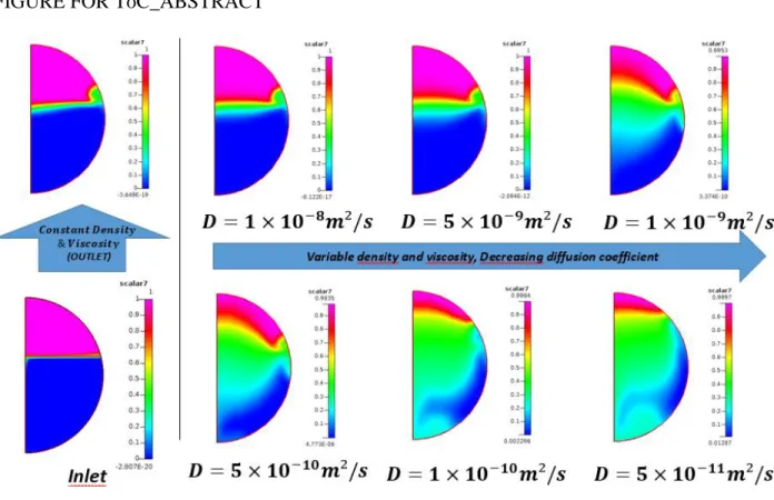
FIGURE FOR ToC_ABSTRACT

3 4 5 6 7 8 9 10 11 12 13 14 15 16 17 18 19 20 21 22 23 24 25 26 27 28 29 30 31 32 33 34 35 36 37 38 39 40 41 42 43 44 45 46 47 48 49 50 51 52 53 54 55 56 57 58 59 60 61 62 63 64 65

3

1. Introduction

Mixing is a very important aspect that needs to be considered before designing any chemical reaction process.[1] In any reactor, improper mixing leads to decrease in the quality of products, lesser production, generation of waste products etc. Moreover, as the size of the reactor increases, the problem of mixing becomes more critical. The mixing can be accomplished in flow reactors either by active or passive methods.[2] The former are those where some moving parts or external source of energy are provided to impart and improve mixing within the reactor, e.g. stirring blades. Whereas in passive methods, mixing is achieved through variations in fluid flow profile generated by geometry of the reactor alone. Active mixing requires huge amount of energy for ensuring desired level of mixing but may be necessary in some cases where high level of mixing needs to be ensured at all times, e.g. for highly viscous reacting fluids etc. Because of the presence of active/moving parts, maintenance cost is an additional burden in active mixing. In some cases, it may not be a good option, e.g. under highly corrosive or fouling environment, frequent maintenance is required which lowers the time productivity. On the other hand, passive mixing is quite simple compared to the active one, it usually requires less energy input for reaching the desired level of mixing. Since, the mixing is achieved due to complex flow profiles generated by specific reactor geometries, various complex geometries have emerged achieving different levels of mixing. However, not all geometries may be good for commercial production.[3]

To ensure the best mixing within the reactor, one simple option would be to have all the reactants mixed before the reaction starts. For batch reactors, all the reagents are usually added to the reactor at low temperature and mixed by means of mechanical stirrers before the temperature being increased to promote the reaction. But for flow reactors, mixing is usually done separately. Mixing at large scale is ensured by forced convection but final mixing happens at molecular level only

3 4 5 6 7 8 9 10 11 12 13 14 15 16 17 18 19 20 21 22 23 24 25 26 27 28 29 30 31 32 33 34 35 36 37 38 39 40 41 42 43 44 45 46 47 48 49 50 51 52 53 54 55 56 57 58 59 60 61 62 63 64 65

4

through diffusion which is a very slow process compared to convection. So to increase mixing, several methods are devised which bring various components close to each other. One way to achieve this is by increasing contact area between the two mixing fluids.[4] Another aspect that affects mixing is the dimensions of the reactor. By decreasing cross-sectional dimensions, contribution of diffusion can become significant in increasing mixing even in laminar flow regime. This is the basis of micromixing and microreactor technology.[2-4]

In this age of computers, Computational Fluid Dynamics (CFD) offers an economical way which enables to evaluate reactor performance without conducting any experiment. All this can be done for different reactor geometries with different flow regimes under different operating conditions. But before running the first simulation, a good mathematical model is required which represents various physical and chemical processes adequately. Depending on the problem, researchers may start with a simple model, compare the results with existing experimental data and then make the model further complex in a step by step manner to encompass all the significant process parameters. Mandal et al.[5] _{have numerically modelled and simulated free radical polymerization (FRP)}

reaction of styrene (St) (30% diluted) using CFD under unmixed feed condition in tubular microreactors of two different geometries. The flow is modelled as Newtonian under laminar regime with constant fluid thermo-physical properties. The two different microreactors are a straight tube reactor (STR) and a coiled flow inverter reactor[6] (CFIR) (Figure 1b and 1d). Compared to STR, CFIR is expected to improve the mixing by two additional processes besides diffusion. First, due to the Dean vortices arising from the curvature in a regular helix and second, due to the rotation of these Dean vortices by 90° when 90° bends are incorporated at regular interval in the main helix.[6] The authors have modelled various chemical species in FRP as passive scalars and have used Zhu Transformation[7] for their normalization to reduce numerical stiffness and numerical errors. The value of diffusion coefficient of different species is kept same and constant

3 4 5 6 7 8 9 10 11 12 13 14 15 16 17 18 19 20 21 22 23 24 25 26 27 28 29 30 31 32 33 34 35 36 37 38 39 40 41 42 43 44 45 46 47 48 49 50 51 52 53 54 55 56 57 58 59 60 61 62 63 64 65

5

for all during a given simulation. Several simulations are carried out against discrete variation of the value of diffusion coefficient. This is done to mimic the effect of viscosity on diffusion and thus mixing.

The results for both microreactors have been compared under same operating conditions but the differences are not very significant as expected. There could be several probable reasons for that. The CFD code requires the chemical data to be converted in mass form from original molar form for various chemical species concentration and kinetic rate coefficients. This leads to the problem of converting the values of kinetic rate coefficients of second order reactions in mass form. Fluid thermo-physical properties (FTPP) like density and viscosity are assumed to be constant for simplifying the modelling in their work. In most of the chemical reactions within same phase, this is generally a good assumption as variation in density and viscosity is not very significant for the given range of conversion. But for polymerization, the viscosity can vary by about 4-6 orders through full conversion[8] thus affecting the flow profile significantly. As a consequence, heat and mass transfers can be decreased severely hence affecting mixing and thus the macromolecular properties i.e. number-average chain length, DPn and polydispersity index, PDI. Besides this, even in physical experiment of polymerization under flow condition, a practical approach of diluting the whole reacting mixture with non-reacting and completely miscible solvent at inlet like 30% linear cut in this case, is used to keep the solution viscosity low. So the easiest approach for modelling this diluted feed could be constant density and viscosity. But modelling density and viscosity as constants actually decouples the otherwise coupled parameters of polymerization reaction, i.e. heat and especially flow profile. Thus this assumption of constant fluid thermo-physical properties needs to be reconsidered to improve the CFD results for simulating FRP in microreactors.

This work is essentially an extension of the work done by Mandal et al.[5] and aims at largely improving the modelling. This extension is achieved by two ways. First, a new transformation[9]

3 4 5 6 7 8 9 10 11 12 13 14 15 16 17 18 19 20 21 22 23 24 25 26 27 28 29 30 31 32 33 34 35 36 37 38 39 40 41 42 43 44 45 46 47 48 49 50 51 52 53 54 55 56 57 58 59 60 61 62 63 64 65

6

(NT) derived recently is used. This NT offers several advantages besides improving CFD results for FRP in microreactor. It enables to feed the CFD code with chemical and kinetic data of FRP in original molar forms for species concentrations and kinetic rate coefficients instead of usual mass form as mentioned earlier. This NT also does not change the form of the equations after transformation hence provides an easier coding and debugging. Second, the variations in FTPP like density, viscosity and thermal conductivity as a function of monomer conversion (XM) are

considered for FRP of methyl methacrylate (MMA). As a consequence, reaction rate, flow, heat transfer and also mixing to some extent are altogether coupled. This improves the modelling and brings it closer to real case. Results are obtained and compared with those for constant properties as in Mandal et al.[5] work. However, the coupling among various physical processes (flow, heat transfer, diffusion) and chemical reaction is not complete as diffusion coefficients of different chemical species is still modelled same and constant. Thus, various CFD simulations are carried out against discrete variation of diffusion coefficient values. The modelling of diffusion coefficient with conversion for each chemical species is quite complex and will lead to convergence problem that can be mitigated only by refining the existing meshing to the point that the convergence will take too much time as well as computational resources unless optimized. Thus it will be taken in a future work.

1.1 Kinetic and Mathematical Model of FRP

The kinetic model of FRP as considered in this work is given in Scheme 1.

Initiator decomposition 𝐼 𝐾→ 2𝑅𝑑 ₀ (a)

Initiation 𝑅0+ 𝑀 𝐾𝑖 → 𝑅1 (b) Propagation 𝑅_𝑛+ 𝑀 𝐾→ 𝑅𝑝 _𝑛+1 (c) Termination by combination 𝑅_𝑛+ 𝑅_𝑚 𝐾→ 𝑃𝑡𝑐 _𝑛+𝑚 (d) 3 4 5 6 7 8 9 10 11 12 13 14 15 16 17 18 19 20 21 22 23 24 25 26 27 28 29 30 31 32 33 34 35 36 37 38 39 40 41 42 43 44 45 46 47 48 49 50 51 52 53 54 55 56 57 58 59 60 61 62 63 64 65

7

Termination by disproportionation 𝑅_𝑛+ 𝑅_𝑚 𝐾→ 𝑃𝑡𝑑 _𝑛+ 𝑃_𝑚 (e)

Transfer to monomer 𝑅_𝑛+ 𝑀 𝐾→ 𝑅𝑓𝑚 ₁+ 𝑃_𝑛 (f)

Scheme 1.- Kinetic scheme for free radical polymerization used in this work

The mathematical model[10] studied in this work is based on the method of moments. 𝜆0, 𝜆1 and 𝜆2

are zeroth, first and second order moments srespectively of the live polymer chain length distribution whereas 𝜇0, 𝜇1 and 𝜇2 are zeroth, first and second order of moments respectively of

dead polymer chains length distribution. The detailed mathematical model of FRP is given in Appendix-A in supplementary Information. Although two more steps, namely the chain transfer to solvent and chain transfer to chain transfer agent steps are also included in mathematical model presented in Appendix-A but they are not considered in this work. This work is general in nature thus inclusion of these two steps could easily be made in future without any special change in the code.

1.2 Mathematical Model for CFD

Following equations are used for CFD problem with chemical reaction and heat effects: The conservation of Mass (incompressible fluid)

∇ ∙ (𝑢) = 0 (1)

The conservation of Momentum –Navier-Stokes equation

𝜌𝜕(𝑢)_𝜕𝑡 + 𝜌 (𝑢 ∙ ∇)𝑢 = −∇𝑝 + ∇ ∙ (𝜂[∇𝑢 + (∇𝑢)𝑇_{]) (2)}

The conservation of Energy with heat generation Q

𝜌𝐶_𝑝𝜕(𝑇)_𝜕𝑡 + 𝜌𝐶_𝑝𝑢 ∙ ∇𝑇 = ∇ ∙ (𝐾∇𝑇) + 𝑄 (3)

where 𝑄 = −∆𝐻_𝑝𝐾_𝑝𝜆₀𝑀 (4)

The conservation of population of Chemical species

3 4 5 6 7 8 9 10 11 12 13 14 15 16 17 18 19 20 21 22 23 24 25 26 27 28 29 30 31 32 33 34 35 36 37 38 39 40 41 42 43 44 45 46 47 48 49 50 51 52 53 54 55 56 57 58 59 60 61 62 63 64 65

8

𝜕𝐶𝑖

𝜕𝑡 + ∇ ∙ (𝐶𝑖𝑢) = ∇ ∙ (𝐷𝑖∇𝐶𝑖 ) + 𝑅𝑖 (5)

The chemical species are modelled as passive scalars and the generation term Ri (Equation (5)) for each chemical species is same as reaction rate term for respective chemical species in batch reactor as presented in detailed mathematical model of FRP in Appendix-A in Supplementary Information.

1.3 New Transformation

The new transformation used in this work is as follows: For concentration terms

For initiator, 𝐼′ = _𝐼𝐼

0 (6)

For monomer, 𝑀′ = _𝑀𝑀

0 (7)

NT is used also for kinetic rate coefficients 𝐾_𝑑′ _{= 𝐾}

𝑑 (8)

𝐾𝑝′ = 𝐾𝑝√𝐼0. 𝑀0 (9)

𝐾_𝑡′_{= 𝐾}

𝑡𝑀0 (10)

All the terms with (‘) are dimensionless in terms of concentration. Some more relationships are given in Appendix-B in Supplementary Information. For details regarding new transformation, please refer to previous work.[9] So, instead of equation (A6) – (A8), equation (B8), (B13) and (B14) respectively are used along with equation (B11) and (B12) in the final mathematical model for CFD.

1.4 Chemical and Kinetic Data

For chemical and kinetic data used for MMA and styrene, please refer to already published work elsewhere.[8,11,12] The reaction conditions are given in Table 1 which are same as taken by Mandal

3 4 5 6 7 8 9 10 11 12 13 14 15 16 17 18 19 20 21 22 23 24 25 26 27 28 29 30 31 32 33 34 35 36 37 38 39 40 41 42 43 44 45 46 47 48 49 50 51 52 53 54 55 56 57 58 59 60 61 62 63 64 65

9

et al.[5] To implement the variations in viscosity, density and thermal conductivity for MMA (Appendix-C) other sources[8,13] are referred.

2. Methodology

All simulations were steady-state simulations only with residence time of 12 hrs. An already proven commercial CFD software package, CFD-ACE+ was used. This CFD package can work well with both structured and unstructured meshing.[9] The geometries studied in this work were the same as used by Mandal et al.[5] Unstructured meshing was used for both straight tube reactor (STR) and coiled flow inverter (CFIR) reactor as shown in Figure 1. The same files for the simulations, as used by Mandal et al.[5]_{, were used in this study so no additional mesh independency tests were}

performed. The reaction conditions for styrene (St) were taken to be also the same. For the case of methyl methacrylate (MMA), all reactor operating conditions were taken same as for St. For running simulation, CFD-ACE and for post-processing, CFD-VIEW were used. The flow, heat and scalar module of CFD-ACE were used to model respective processes.

Five passive scalars were used for modelling different chemical species. Scalar1 represented initiator concentration whose generation term was defined by equation (A1). Similarly, Scalar2 represented monomer concentration with equation (A2), Scalar3-Scalar5 are for 𝜇0, 𝜇1 & 𝜇2

through equation (A9)-(A11) respectively. Diffusion coefficient was taken to be same for all these chemical species (Scalar1-5) in a given CFD simulation. The diffusion coefficient was varied discretely for the CFD simulations (Table 1). Besides these five passive scalars, two additional passive scalars were also used to represent inert tracer and to qualitatively observe the process of mixing with and without diffusion in the current work. Of these, one passive scalar modelled diffusing tracer while the other modelled non-diffusing tracer. The former passive scalar i.e. diffusing inert tracer was denoted as Scalar6 whereas non-diffusing inert tracer was denoted as

3 4 5 6 7 8 9 10 11 12 13 14 15 16 17 18 19 20 21 22 23 24 25 26 27 28 29 30 31 32 33 34 35 36 37 38 39 40 41 42 43 44 45 46 47 48 49 50 51 52 53 54 55 56 57 58 59 60 61 62 63 64 65

10

Scalar7. For non-diffusing inert tracer (Scalar7), the diffusion coefficient was taken to be 1x10-20 for all simulations. For the diffusing inert tracer (Scalar6), the diffusion coefficient was taken to be the same as that for all other chemical species in that simulation. This was done to observe the mixing effect due to diffusion at same reference level of diffusion of other reacting chemical species.

Scalar6 modelled solvent also when variation in FTPP is conisdered. In one set of CFD simulations, the FTPP like density, viscosity, thermal conductivity and specific heat were kept constant to their values as reported in Table 1 for both MMA and St. Other set of CFD simulations was carried out for MMA only in which density, thermal conductivity and fluid viscosity were varied by using the expressions given in Baillagou and Soong.[8]

Velocity and concentration profiles were modelled flat at the inlet. The inlet as well as wall temperatures were taken to be 70°C. No-slip at walls, zero flux for all the passive scalars across the wall and isothermal condition at wall were taken as boundary conditions. The flow was modelled as Newtonian. The fluids at inlet (solvent + initiator and monomer) were considered to be totally miscible in each other and to have similar properties. The monomer was fed from the bigger cut of inlet and initiator with solvent was fed from smaller (30%) cut of inlet. Inlet values for scalars are given in Table 2.

To prevent wrong calculation of viscosity based on monomer conversion, following scheme was used. In any cell, if the Scalar6 (solvent as non-reacting diffusing tracer) is 1, i.e. only solvent is present, then volume fraction of monomer in that cell was taken to be 0. If Scalar6 value is zero, i.e. the solvent is absent, then XM and volume fraction are to be obtained for bulk polymerization.

For all other cases, XM and volume fraction were calculated for solution polymerization with

constant dilution factor equal to 0.3.

3 4 5 6 7 8 9 10 11 12 13 14 15 16 17 18 19 20 21 22 23 24 25 26 27 28 29 30 31 32 33 34 35 36 37 38 39 40 41 42 43 44 45 46 47 48 49 50 51 52 53 54 55 56 57 58 59 60 61 62 63 64 65

11

Third order spatial discretization scheme was used for velocity, enthalpy and especially all passive scalars to minimize the numerical diffusion. SIMPLEC was used for pressure-velocity coupling. Algebraic MultiGrid (AMG) solver was used for pressure. Conjugated gradient squared (CGS) + preconditioning solver was used for velocity, enthalpy and all passive scalars. The simulations were assumed to have converged when the residual error ratio reduced below 10-8 for all the variables. Various relaxation parameters related to velocity, pressure etc. and all passive scalars were adjusted to make the simulations converge faster as well as below the above mentioned limit of residual error ratio for all variables. Simulations with different values of diffusion coefficient required different values of relaxation parameters to make the simulation converged.

3. Results and Discussion

By optimizing different relaxation parameters, we have been able to get the simulations converged faster (mostly in about 150-3000 iterations depending on the value of the diffusion coefficient) for most of the variables. Along with this, we even got much lower residual error ratio values than the criteria we had set and with an extended range of diffusion coefficient values compared to Mandal et al.[5] Furthermore, the new transformation is applied successfully and all data are fed in molar form only. Plots of various variables are presented against diffusion coefficient on semi-log plot with x-axis in log scale for the ease of presentation.

Figure 2 to Figure 4 show the results regarding XM, DPn and PDI respectively for both STR and

CFIR obtained in this work for constant FTPP and compared with Mandal et al.[5] under similar conditions.

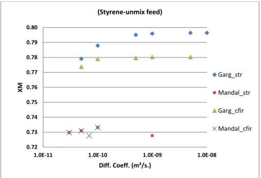
In Figure 2, it can easily be seen that XM has been calculated higher for both STR and CFIR in

current work compared to Mandal et al.[5] _{This result is in accordance with the results obtained in}

our previous work on NT.[9] Using the kinetics rate expressions obtained for molar form while

3 4 5 6 7 8 9 10 11 12 13 14 15 16 17 18 19 20 21 22 23 24 25 26 27 28 29 30 31 32 33 34 35 36 37 38 39 40 41 42 43 44 45 46 47 48 49 50 51 52 53 54 55 56 57 58 59 60 61 62 63 64 65

12

feeding the data for monomer and initiator concentrations as well as kinetic rate coefficients in mass form introduces a significant error in CFD simulation. This problem is bypassed by NT as fed data remain in molar form and thus avoids such error.

Besides this, XM is predicted consistently higher for STR compared to CFIR in current work. This

can be understood easily by looking at the inlet feed condition. Since the two reactant streams (solvent + initiator and monomer) are fed to the reactor in unmixed condition (Figure 1c), they can only be mixed along the reactor with flow. Since the initiator is mixed with solvent and not with monomer, so monomer and initiator (with solvent) need to diffuse in opposite regions to promote any reaction. In STR, the mixing operates solely because of diffusion process, so the concentration of monomer remains high at interface which favours a rapid polymerization rate. Thus higher monomer concentration leads to higher XM.[14] In CFIR, the mixing is enhanced by secondary flows

(Dean Vortices) as well as by inversion of secondary flows due to the 90° bends at regular intervals in curved geometry (helical shape).[6] Although the secondary flows will be very small but they will still improve mixing as shown by Vanka et al.[15] _{for non-viscous fluids. This along with}

diffusion process lowers the monomer concentration for reaction and thus lower XM is achieved.

The XM in Figure 2 can also be observed to be increasing with an increase in diffusion coefficient

and then remains nearly constant for high diffusion coefficients. This is because increasing diffusion coefficient increases the mixing process by diffusion and hence after a certain value of diffusion coefficient for a given reactor dimension and velocity (as given by Peclet number), mixing remains same and concentration remains uniform throughout the cross-section. For STR, the variation in XM from low values of diffusion coefficient to high values is quite significant

compared to CFIR. This clearly shows the improved internal mixing in CFIR which is its clear benefit over STR for XM even at low values of diffusion coefficient.

3 4 5 6 7 8 9 10 11 12 13 14 15 16 17 18 19 20 21 22 23 24 25 26 27 28 29 30 31 32 33 34 35 36 37 38 39 40 41 42 43 44 45 46 47 48 49 50 51 52 53 54 55 56 57 58 59 60 61 62 63 64 65

13

Compared to current work, the results obtained by Mandal et al.[5] do not show significant differences for XM between STR and CFIR. Moreover, due to smaller range of diffusion coefficient

values in their simulations, no trend could be figured out.

It is noteworthy to mention that higher XM in STR will not come without disadvantages. Due to

poor mixing and higher XM in STR, DPn and PDI should be affected in a negative way. DPn should

be lower whereas PDI should be higher compared to CFIR. As shown in Figure 3 and Figure 4 respectively for DPn and PDI, it can be observed that this is indeed the case. Here, significant observation about the difference in values of DPn for CFIR and STR for the same range of values of diffusion coefficient could be made. The values of DPn for CFIR are nearly twice as much compared to STR as shown in Figure 3. This is a significant improvement over STR. Besides this, for CFIR, the value of DPn is nearly constant for the whole range of diffusion coefficient whereas for STR, it increases for low values of diffusion coefficient. Besides this, again one can observe that the DPn in current work for both STR and CFIR are predicted significantly higher compared to those obtained by Mandal et al.[5] _{It is also on the same line as shown in our previous work about}

NT. It is also shown in the same previous work that DPn is strongly dependent on the initial numerical values of both the initiator and monomer (equation. B22). Hence the units and thus the numerical values fed to the CFD code are very important to provide a good prediction of DPn. Therefore, the values of DPn predicted using NT are nearer to experimental values. So, these results in current work regarding DPn are more reliable. CFIR is thus shown to have much better control on DPn compared to STR for same range of variation of diffusion coefficients.

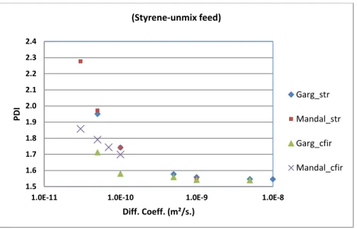
In Figure 4, it can be observed that PDI values for STR in current work match well with Mandal et al.[5] There, PDI is shown to be independent of initial concentrations of initiator and monomer (equation. B23) and thus unaffected by units (mass or molar). Subsequently it is shown that in absence of any convective mixing and presence of diffusion alone as in STR, PDI results in CFD

3 4 5 6 7 8 9 10 11 12 13 14 15 16 17 18 19 20 21 22 23 24 25 26 27 28 29 30 31 32 33 34 35 36 37 38 39 40 41 42 43 44 45 46 47 48 49 50 51 52 53 54 55 56 57 58 59 60 61 62 63 64 65

14

using NT will match with those obtained using Zhu transformation[7]. Figure 4 for PDI actually proves that the results shown in current work are in right direction. If the modelling in current work had been wrong, then this matching would not have occurred.

It can also be seen that PDI predicted for CFIR is lower than STR in both current and Mandal et al.[5] works. This is due to improved mixing as explained earlier. In addition to that, it can be seen that PDI for CFIR predicted in current work remains nearly constant for a larger range of diffusion coefficients. Besides this, variation in PDI values for CFIR is much less compared to STR for the same range of diffusion coefficient. For higher diffusion coefficients, PDI for both STR and CFIR are nearly the same. This again is due to improved mixing resulting from higher diffusion coefficients and hence lower Peclet numbers. This result demonstrates the improved control over PDI by CFIR compared to STR under similar conditions.

Figure 2 to Figure 4 clearly present the significant improvements gained in current work compared

to previous work by Mandal et al.[5] under same conditions with constant FTPP. With this simplified modelling, current work has been able to show in a better manner with more clarity the superiority of CFIR over STR.

Results for MMA simulated under similar conditions are presented in Figure 5 to Figure 9. These results have been obtained for constant (decoupled processes case) as well as with variation in density, viscosity and thermal conductivity with discrete variation of diffusion coefficient. This is done to couple reaction, flow and heat transfer processes, and hence to observe the impact of these physical properties on flow and thus on mixing. In each figure, the data are presented for both STR and CFIR for both constant and variable FTPP.

Figure 5 shows the results for XM. Similar to the results obtained for styrene, XM in STR is

predicted to be higher compared to CFIR. This observation is same for both cases of constant and variable FTPP. It can also be observed that predictions for XM are slightly shifted to higher values

3 4 5 6 7 8 9 10 11 12 13 14 15 16 17 18 19 20 21 22 23 24 25 26 27 28 29 30 31 32 33 34 35 36 37 38 39 40 41 42 43 44 45 46 47 48 49 50 51 52 53 54 55 56 57 58 59 60 61 62 63 64 65

15

for variable FTPP compared to constant ones. It can be explained this way. The modelling of the variation of FTPP couples flow to chemical reaction through density and viscosity which are function of conversion and temperature. Hence flow profile gets affected by the localized rate of chemical reaction which in turns affects the localized rate of heat generation and conversion. This affects the mixing of the fluid and hence affects the local monomer concentration. This local variation of monomer concentration affects the localized rate of chemical reaction and this cycle goes-on. Thus the modelling of the FTPP as a function of temperature and conversion actually models the coupling of the different aforementioned processes. This will also increase residence time in highly viscous zones and hence more conversion is expected in these zones thus raising overall conversion. This is nearer to physical reality and hence accounts for the mixing within the microreactor in a better way. Therefore it affects and improves XM prediction through CFD

simulations significantly.

Figure 6 shows the results for DPn. Here again the predictions for variable FTPP (coupled case)

are higher compared to the case of constant one (decoupled case). Moreover, for both CFIR and STR, DPn increases when diffusion coefficient increases. This could be due to decreased conversion at lower diffusion coefficient originating from an increased viscosity with conversion. The same can be observed by less viscosity at STR outlet for lower diffusion coefficient compared to higher values of diffusion coefficient in Table 4. Besides this, the results for CFIR are better than STR whether the coupling of the process is modelled or not.

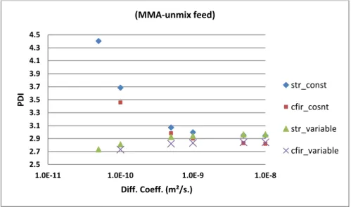
Figure 7 shows the results for PDI. It shows the most significant difference between constant

(decoupled case) and variable FTPP case (coupled case). For constant parameters, PDI is increasing for both STR and CFIR when the value of diffusion coefficient is decreasing. Similar trend is reported earlier for STR for constant FTPP case.[5,16] One can expect lower mixing for low diffusion coefficients and thus higher PDI due to poor mixing. Whereas, for coupled processes case, PDI

3 4 5 6 7 8 9 10 11 12 13 14 15 16 17 18 19 20 21 22 23 24 25 26 27 28 29 30 31 32 33 34 35 36 37 38 39 40 41 42 43 44 45 46 47 48 49 50 51 52 53 54 55 56 57 58 59 60 61 62 63 64 65

16

decreases with decrease in the value of diffusion coefficient. This result seems to be unexpected. Ivleva et al.[17] have discussed the conditions under which chemical reactions promote mixing in unstirred reactor. In one case they have discussed about increased mixing due to natural convection originating from spatial temperature variations. This spatial temperature variation arises out of non-uniformity in reaction rate and cooling rates through reactor walls. Another case discussed by the same authors concerned the increased mixing due to chaotic behavior in certain chemical reactions. These chemical reactions have several elementary steps which may proceed in a chaotic way spatially. Hence, it can lead to local variations of temperature, conversion and FTPP like density, viscosity etc. This may induce convective mixing due to buoyancy effect etc. and hence improved mixing. So in current case, the reason comes from the situation where unmixed feed condition is coupled with the variation of FTPP. The probable explanation is as follows. Due to the decreasing value of the diffusion coefficient, the diffusion of monomer and solvent (and thus initiator) towards each other is reduced. Thus, reaction becomes more non-uniform across the cross-section of the reactor. This leads to non-uniform XM across the cross-section as well as axially. Since the viscosity

is a function of XM through volume fraction of monomer and polymer,[8] this will lead to

non-uniformity of viscosity across the cross-section. This, when combined with variation in density due to XM (density will increase due to polymer formation), will affect the local flow profile and will

bend the streamlines locally increasing local mixing. This will thus improve mixing even in STR instead of decreasing it.

The same analysis can also explain the increased mixing of Scalar7 (non-reacting non-diffusing tracer) at lower diffusion coefficients compared to low or no mixing at higher diffusion coefficients as shown in Table 3. Scalar7 cannot mix by diffusion due to its very low value of diffusion coefficient. So it can mix only by convective mixing (i.e. by flow). At higher diffusion coefficient, the mixing between solvent (and thus initiator) and monomer is improved and thus radial

3 4 5 6 7 8 9 10 11 12 13 14 15 16 17 18 19 20 21 22 23 24 25 26 27 28 29 30 31 32 33 34 35 36 37 38 39 40 41 42 43 44 45 46 47 48 49 50 51 52 53 54 55 56 57 58 59 60 61 62 63 64 65

17

conversion is nearly uniform. Hence the variation in density and viscosity across the cross-section is less and thus the flow profile remains nearly unchanged. Scalar7 remains unmixed and non-diffused at high values of diffusion coefficients in the absence of any convective flow across cross-section which occurs at low value of diffusion coefficient as explained earlier. The broadening of Scalar7 concentration at the mixing interface in STR is due to the coarser mesh used.

In CFIR, the Scalar7 profile looks same but maximum and minimum concentration values as shown in respective graphs are different. CFIR with variable FTPP shows much higher mixing of Scalar7 at all diffusion coefficient values as inferred by much lower difference between maximum and minimum values of concentration. This shows that CFIR improves mixing even for highly non-diffusing components even at such a low inlet Reynolds number of 0.06.

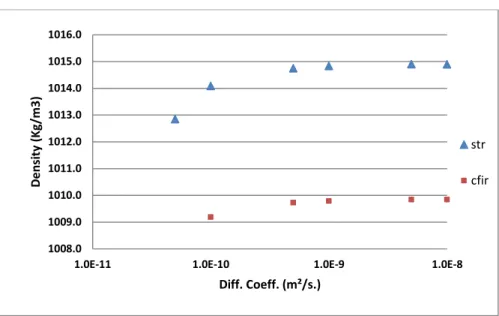
Figure 8 and Figure 9 show the variation of fluid density and viscosity respectively at the reactor

outlet for both STR and CFIR. The trend can easily be related to the increase in XM with respect to

diffusion coefficient as shown in Figure 5. Higher XM means higher density and viscosity. The

viscosity is found to rise by 6 orders from inlet to outlet during the simulations. The density and viscosity distribution at reactor outlet can also be seen in Table 4 for both STR and CFIR at different diffusion coefficients. Higher density and viscosity can be observed near wall. This is due to the fact that no-slip boundary condition is applied at wall. So residence time is higher near the wall. This led to higher conversion at wall compared to the center of the tube. The same can be observed for Scalar2 at outlet as shown in Table 5. The distribution of density, viscosity as well as Scalar2 can be observed to be much more uniform in CFIR compared to STR proving that the mixing in CFIR is much better than STR even in case of variable FTPP. The asymmetric radial distribution of density, viscosity (Table 4) and Scalar2 (Table 5) at CFIR outlet clearly points out the presence of secondary flows even at such a low inlet Reynolds number.

3 4 5 6 7 8 9 10 11 12 13 14 15 16 17 18 19 20 21 22 23 24 25 26 27 28 29 30 31 32 33 34 35 36 37 38 39 40 41 42 43 44 45 46 47 48 49 50 51 52 53 54 55 56 57 58 59 60 61 62 63 64 65

18

Despite huge variation in viscosity and moderate changes in density, no significant variation of thermal conductivity is observed. The temperature variation across the cross section differs only by 0.1K even after varying FTPP. Thus truly isothermal condition is observed even during high viscosity variation and density changes. So, modelling thermal conductivity as constant would be a good assumption without affecting any simulation results.

Table 6 shows the scalar6 profile at the outlet of STR and CFIR for both varying and constant

FTPP. Scalar6 represents a non-reacting diffusing tracer. It is observed to be uniformly spread across the reactor cross-section when the diffusion coefficient is increasing even for STR. This is in contrast to the profile of Scalar7 which is a non-reacting and non-diffusing tracer. This shows that due to its small cross-sectional dimensions, complete mixing can be achieved for diffusing components even in STR (where convective mixing is absent under laminar flow). Another interesting observation is that CFIR achieves the complete mixing for Scalar6 even at lower value of diffusion coefficient compared to STR despite having same dimensions and operating conditions. This shows again the better mixing capabilities of CFIR over STR under similar conditions.

4. Conclusions

FRP is modelled and simulated in two different microtubular geometries namely STR and CFIR under unmixed feed condition. A new transformation is applied which allows feeding chemical species concentration and kinetic rate coefficients data in molar form instead of mass form by rendering the equations dimensionless in terms of concentration. Results are first compared with the existing work of Mandal et al.[5] obtained for styrene and for constant FTPP (density, viscosity, thermal conductivity) i.e. flow, reaction, and heat transfer are decoupled during modelling. Significant differences between the two works are observed. Compared to Mandal et al.,[5] current

3 4 5 6 7 8 9 10 11 12 13 14 15 16 17 18 19 20 21 22 23 24 25 26 27 28 29 30 31 32 33 34 35 36 37 38 39 40 41 42 43 44 45 46 47 48 49 50 51 52 53 54 55 56 57 58 59 60 61 62 63 64 65

19

work predicts higher XM and higher DPn for both STR and CFIR while predicting PDI lower for

CFIR. But prediction of PDI for STR remained same due to the new transformation. Compared to STR, CFIR shows much higher DPn with lower PDI. But the XM is slightly lower compared to

STR. The modelling is then extended to include the variation in FTPP which couples the above mentioned processes and hence accounts better for the actual physical process. MMA is selected for this and the results are evaluated under the conditions similar to those applied for styrene. Compared to decoupled case (constant variables) with coupled case (variable fluid thermo-physical properties), the results for XM and DPn are found to be on higher side with similar trend for coupled

case. But for PDI, the values are found to be lower with different trends especially at lower diffusion coefficient in coupled case. A special case of increased mixing in STR at low diffusion coefficient for unmixed feed condition is observed for coupled case which cannot be observed otherwise with decoupled case. This clearly emphasizes the importance of modelling coupling of various parameters to properly account for the real thermo-physical-chemical process of FRP in tubular microreactor under unmixed feed condition. CFIR is found to have a much better mixing capability and thus has the possibility to promote a better control over DPn and PDI of the produced polymer compare to STR under similar conditions for unmixed feed condition. Thermal conductivity variation and temperature variation across the cross section of the tube are found to be negligible even in the case of variable FTPP. Hence thermal conductivity can be modelled as constant without any significant effect on the results. Reaction can be assumed to be isothermal for all conditions investigated.

Supporting Information

Supporting Information is available from the Wiley Online Library

Appendix-A:

3 4 5 6 7 8 9 10 11 12 13 14 15 16 17 18 19 20 21 22 23 24 25 26 27 28 29 30 31 32 33 34 35 36 37 38 39 40 41 42 43 44 45 46 47 48 49 50 51 52 53 54 55 56 57 58 59 60 61 62 63 64 65

20

Appendix-B: Zhu Transformation and New transformation

Appendix-C:

Nomenclature

𝐴𝐻 Area for heat transfer, 𝑚2

𝐶_{𝑀 =}𝐾𝑓𝑚

𝐾𝑝 , dimensionless

𝐶𝑝 Specific heat capacity of mixture, cal/g/°C 𝐶𝑇 =𝐾𝑡𝑑

𝐾𝑡𝑐, dimensionless

𝐷𝑃𝑛 Number averaged degree of polymerization

𝐼 Initiator concentration, mol/l 𝐾_𝑑 Dissociation rate coefficient, min-1

𝐾_𝑓𝑚 Transfer to monomer rate coefficient, l/(mol.min) 𝐾𝑖 Kinetic rate constant for initiation, s-1

𝐾_𝑝 Propagation rate coefficient, l/(mol.min) 𝐾_𝑝𝑟 = 𝐾_𝑝+ 𝐾_𝑓𝑚= (1 + 𝐶_𝑀)𝐾_𝑝, l/(mol.min)

𝐾𝑡 = 𝐾𝑡𝑐+ 𝐾𝑡𝑑, l/(mol.min)

𝐾_𝑡𝑐 Termination by combination rate coefficient, l/(mol.min) 𝐾_𝑡𝑑 Termination by disproportionation rate coefficient, l/(mol.min)

𝐿 _{Kinetic chain length, =} 𝐾𝑝𝑟𝑀𝜆0 2𝑓𝐾𝑑𝐼

𝐿̅ _{= 𝐿. (}1− 𝑅𝑀𝑀

1+ 𝑅𝑃𝐿) = 𝐿. ( 1− 𝑅𝑀 1+ 𝑅𝑃𝐿)

𝑀 Monomer concentration, mol/l

3 4 5 6 7 8 9 10 11 12 13 14 15 16 17 18 19 20 21 22 23 24 25 26 27 28 29 30 31 32 33 34 35 36 37 38 39 40 41 42 43 44 45 46 47 48 49 50 51 52 53 54 55 56 57 58 59 60 61 62 63 64 65

21 𝑀𝑊 Molecular weight, g/mol

𝑀𝑊𝑛 Number averaged chain length of polymer, g/mol

𝑀𝑊𝑤 Weight averaged chain length of polymer, g/mol

𝑃𝐷𝐼 Polydispersity index, dimensionless

𝑃_𝑛 Dead polymer chain length of n no. of monomer units 𝑅 Universal gas constant, 1.986 cal/mol/K

𝑅₀ Zero order radical obtained from initiator dissociation

𝑅𝑀 = 𝐾𝑓𝑚 𝐾𝑝+𝐾𝑓𝑚 = 𝐾𝑓𝑚 𝐾𝑝𝑟 = 𝐶𝑀 1+𝐶𝑀 𝑅_𝑀𝑀 = 𝑅_𝑀

𝑅𝑛 Live polymer chain length of n no. of monomer units

𝑅𝑇 = 𝐾𝑡𝑐 𝐾𝑡𝑐+ 𝐾𝑡𝑑= 𝐾𝑡𝑐 𝐾𝑡 = 1 1+𝐶𝑇, dimensionless 𝑇 Temperature, K

𝑇_{𝑏𝑎𝑡ℎ} Temperature of heat sink, K

𝑈 Overall heat transfer coefficient, W/m2_/K

𝑉𝑅 Volume of solution at any time t, liter

𝑉𝑅0 Initial volume of solution at t0, liter

𝑋_𝑀 Monomer conversion, dimensionless 𝑓 Initiator efficiency, dimensionless

𝑓_𝑠 Initial Solvent volume fraction, dimensionless 𝑓𝑣 Fractional free volume, dimensionless

𝑡 Time , min u Velocity, m/s 3 4 5 6 7 8 9 10 11 12 13 14 15 16 17 18 19 20 21 22 23 24 25 26 27 28 29 30 31 32 33 34 35 36 37 38 39 40 41 42 43 44 45 46 47 48 49 50 51 52 53 54 55 56 57 58 59 60 61 62 63 64 65

22 ∆𝐻_𝑃 Heat of reaction, cal/mol

𝛽 Ratio of solvent volume to non-solvent volume, dimensionless

𝜀 Volume contraction factor corrected for solvent volume fraction, dimensionless 𝜀₀ Volume contraction factor without solvent volume fraction, dimensionless 𝜆₀ Zeroth order moment for live polymer chain length distribution, mol/l 𝜆₁ First order moment for live polymer chain length distribution, mol/l 𝜆₂ Second order moment for live polymer chain length distribution, mol/l 𝜇0 Zeroth order moment for dead polymer chain length distribution, mol/l

𝜇₁ First order moment for dead polymer chain length distribution, mol/l 𝜇₂ Second order moment for dead polymer chain length distribution, mol/l

𝜌 Mixture density, g/cm3

𝛷 Volume fraction, dimensionless 𝜂 Dynamic viscosity, cP Subscript 𝑀 Monomer 𝑃 Polymer 𝑆 Solvent 𝐼 Initiator 0 At time t=0

Acknowledgements: The financial support by ANR grant No. 09-CP2D-DIP² is greatly appreciated. 3 4 5 6 7 8 9 10 11 12 13 14 15 16 17 18 19 20 21 22 23 24 25 26 27 28 29 30 31 32 33 34 35 36 37 38 39 40 41 42 43 44 45 46 47 48 49 50 51 52 53 54 55 56 57 58 59 60 61 62 63 64 65

23

Keywords: coupled problem, CFD, mixing, free radical polymerization, coiled flow inverter microreactor

[1] O. Levenspiel, Chemical Reaction Engineering, 3rd ed., John Wiley & Sons, New York, 1999.

[2] V. Hessel, H. Lowe, F. Schonfeld, Chem Eng Sci, 2005, 60 (8-9), 2479-2501. [3] Y. K. Suh, S. Kang, Micromachines, 2010, 1 (3), 82-111.

[4] H. Bockhorn, D. Mewes, W. Peukert, H.-J. Warnecke, Micro and Macro Mixing:

Analysis, Simulation and Numerical Calculation, Springer-Verlag Berlin Heidelberg: Berlin,

Heidelberg, 2010.

[5] M. M. Mandal, C. Serra, Y. Hoarau, K. D. P. Nigam, Microfluid Nanofluid, 2011, 10

(2), 415-423.

[6] a) A. K. Saxena, K. D. P. Nigam, AIChE J, 1984, 30 (3), 363-368; b) E. López-Guajardoa, E. Ortiz-Nadala, A. Montesinos-Castellanosa, K. D. P. Nigam, Chem. Eng. Sci.,2017, 169, 179-185; c) M. Schmalenberg, W. Krieger, N. Kockmann, Chemie Ingenieur Technik, 2019, 91 (5), 567-575.

[7] S. Zhu Macromol Theor Simul, 1999, 8 (1), 29–37

[8] P. E. Baillagou, D. S. Soong, Polym Eng Sci, 1985, 25 (4), 212-231.

[9] D. K. Garg, C. A. Serra, Y. Hoarau, D. Parida, M. Bouquey, R. Muller, Microfluid

Nanofluid, 2014, 18 (5-6), 1287-1297.

[10] D. K. Garg, C. A. Serra, Y. Hoarau, D. Parida, M. Bouquey, R. Muller,

Macromolecules, 2014, 47 (14), 4567-4586.

[11] A. Keramopoulos, C. Kiparissides, J Appl Polym Sci, 2003, 88 (1), 161-176. [12] A. Keramopoulos, C. Kiparissides, Macromolecules, 2002, 35 (10), 4155-4166.

3 4 5 6 7 8 9 10 11 12 13 14 15 16 17 18 19 20 21 22 23 24 25 26 27 28 29 30 31 32 33 34 35 36 37 38 39 40 41 42 43 44 45 46 47 48 49 50 51 52 53 54 55 56 57 58 59 60 61 62 63 64 65

24

[13] R. H. Shoulberg, J. A. Shetter, J. Appl. Polym. Sci., 1962, 23 (6), 32-33.

[14] B. Cortese, T. Noel, M. H. J. M. de Croon, S. Schulze, E. Klemm, V. Hessel, Macromol

React Eng, 2012, 6 (12), 507-515.

[15] S. P. Vanka, G. Luo, C. M. Winkler, Aiche J, 2004, 50 (10), 2359-2368.

[16] C. Serra, G. Schlatter, N. Sary, F. Schonfeld, G. Hadziioannou, Microfluid Nanofluid,

2007, 3 (4), 451-461.

[17] T. P. Ivleva, A. G. Merzhanov, E. N. Rumanov, N. I. Vaganova, A. N. Campbell, A. N. Hayhurst, Chem Eng J, 2011, 168 (1), 1-14.

3 4 5 6 7 8 9 10 11 12 13 14 15 16 17 18 19 20 21 22 23 24 25 26 27 28 29 30 31 32 33 34 35 36 37 38 39 40 41 42 43 44 45 46 47 48 49 50 51 52 53 54 55 56 57 58 59 60 61 62 63 64 65

25

(a) (c)

b) (d)

(e)

Figure 1. a) meshing for inlet of STR,[5] b) volume grid of STR,[5] c) meshing of inlet of coil flow inverter reactor[5] (CFIR), d) general view of CFIR,[5] e) detailed view of volume grid of CFIR[5]

3 4 5 6 7 8 9 10 11 12 13 14 15 16 17 18 19 20 21 22 23 24 25 26 27 28 29 30 31 32 33 34 35 36 37 38 39 40 41 42 43 44 45 46 47 48 49 50 51 52 53 54 55 56 57 58 59 60 61 62 63 64 65

26

Figure 2. Variation of St conversion (𝑋_𝑀) with diffusion coefficient for the case of constant fluid thermo-physical properties.

Figure 3. Variation of polystyrene number-average chain length with diffusion coefficient for the

case of constant fluid thermo-physical properties.

0.72 0.73 0.74 0.75 0.76 0.77 0.78 0.79 0.80

1.0E-11 1.0E-10 1.0E-09 1.0E-08

XM Diff. Coeff. (m²/s.) (Styrene-unmix feed) Garg_str Mandal_str Garg_cfir Mandal_cfir 0 200 400 600 800 1000 1200 1400

1.0E-11 1.0E-10 1.0E-9 1.0E-8

D Pn Diff. Coeff. (m²/s.) (Styrene-unmix feed) Garg_str Mandal_str Garg_cfir Mandal_cfir 3 4 5 6 7 8 9 10 11 12 13 14 15 16 17 18 19 20 21 22 23 24 25 26 27 28 29 30 31 32 33 34 35 36 37 38 39 40 41 42 43 44 45 46 47 48 49 50 51 52 53 54 55 56 57 58 59 60 61 62 63 64 65

27

Figure 4. Variation of polystyrene polydispersity index with diffusion coefficient for the case of

fluid constant fluid thermo-physical properties.

Figure 5. Variation of MMA conversion (𝑋_𝑀) with diffusion coefficient for constant as well as variable fluid thermo-physical properties.

1.5 1.6 1.7 1.8 1.9 2.0 2.1 2.2 2.3 2.4

1.0E-11 1.0E-10 1.0E-9 1.0E-8

PDI Diff. Coeff. (m²/s.) (Styrene-unmix feed) Garg_str Mandal_str Garg_cfir Mandal_cfir 0.95 0.96 0.97 0.98

1.0E-11 1.0E-10 1.0E-9 1.0E-8

XM Diff. Coeff. (m²/s.) (MMA-unmix feed) str_const cfir_cosnt str_variable cfir_variable 3 4 5 6 7 8 9 10 11 12 13 14 15 16 17 18 19 20 21 22 23 24 25 26 27 28 29 30 31 32 33 34 35 36 37 38 39 40 41 42 43 44 45 46 47 48 49 50 51 52 53 54 55 56 57 58 59 60 61 62 63 64 65

28

Figure 6. Variation of poly(methyl methacrylate) number-average chain length, DPn with

diffusion coefficient for constant as well as variable fluid thermo-physical properties.

Figure 7. Variation of poly(methyl methacrylate) polydispersity index with diffusion coefficient

for constant as well as variable fluid thermo-physical properties.

1290 1300 1310 1320 1330 1340 1350 1360 1370 1380 1390

1.0E-11 1.0E-10 1.0E-9 1.0E-8

D Pn Diff. Coeff. (m²/s.) (MMA-unmix feed) str_const cfir_cosnt str_variable cfir_variable 2.5 2.7 2.9 3.1 3.3 3.5 3.7 3.9 4.1 4.3 4.5

1.0E-11 1.0E-10 1.0E-9 1.0E-8

PDI Diff. Coeff. (m²/s.) (MMA-unmix feed) str_const cfir_cosnt str_variable cfir_variable 3 4 5 6 7 8 9 10 11 12 13 14 15 16 17 18 19 20 21 22 23 24 25 26 27 28 29 30 31 32 33 34 35 36 37 38 39 40 41 42 43 44 45 46 47 48 49 50 51 52 53 54 55 56 57 58 59 60 61 62 63 64 65

29

Figure 8. Variation of fluid density with diffusion coefficient for MMA.

Figure 9. Variation of fluid viscosity with diffusion coefficient for MMA. 1008.0 1009.0 1010.0 1011.0 1012.0 1013.0 1014.0 1015.0 1016.0

1.0E-11 1.0E-10 1.0E-9 1.0E-8

D e n si ty ( Kg /m3) Diff. Coeff. (m²/s.) str cfir 25.0 30.0 35.0 40.0 45.0 50.0

1.0E-11 1.0E-10 1.0E-9 1.0E-8

V isc o si ty ( Pa.s) Diff. Coeff. (m²/s.) str cfir 3 4 5 6 7 8 9 10 11 12 13 14 15 16 17 18 19 20 21 22 23 24 25 26 27 28 29 30 31 32 33 34 35 36 37 38 39 40 41 42 43 44 45 46 47 48 49 50 51 52 53 54 55 56 57 58 59 60 61 62 63 64 65

30

Table 1. Operating conditions and physical data for constant FTPP [5]

Wall temperature (K) - constant 343

Chemical species diffusion coefficient. (m2/s) from 3×10−12 to 1×10−8

Fluid density(kg/m3) 1×103

Fluid viscosity (Pa.s) 1×10−3

Fluid thermal conductivity (W/m/K) 0.6

Fluid specific heat (J/kg/K) 4182

Fluid velocity (m/s) 2.9×10−5

Inlet Reynolds number 0.06

Residence time (hrs) 12

Table 2. Scalar values at reactor inlet for unmixed condition.

70% cut 30% cut Scalar1 0 1 Scalar2 1 0 Scalar3-5 0 0 Scalar6-7 0 1 3 4 5 6 7 8 9 10 11 12 13 14 15 16 17 18 19 20 21 22 23 24 25 26 27 28 29 30 31 32 33 34 35 36 37 38 39 40 41 42 43 44 45 46 47 48 49 50 51 52 53 54 55 56 57 58 59 60 61 62 63 64 65

31

Table 3. Scalar7 distribution at reactor outlet.

Diffusion coefficient (m²/s) STR CFIR Constant parameters Variable parameters

Constant parameters Variable parameters

𝟓 × 𝟏𝟎−𝟏𝟏 𝟏 × 𝟏𝟎−𝟏𝟎 𝟓 × 𝟏𝟎−𝟏𝟎 𝟏 × 𝟏𝟎−𝟗 𝟓 × 𝟏𝟎−𝟗 𝟏 × 𝟏𝟎−𝟖 3 4 5 6 7 8 9 10 11 12 13 14 15 16 17 18 19 20 21 22 23 24 25 26 27 28 29 30 31 32 33 34 35 36 37 38 39 40 41 42 43 44 45 46 47 48 49 50 51 52 53 54 55 56 57 58 59 60 61 62 63 64 65

32

Table 4. Density and viscosity at reactor outlet

Density Viscosity Diffusion coefficient (m²/s) STR CFIR STR CFIR 𝟓 × 𝟏𝟎−𝟏𝟏 𝟏 × 𝟏𝟎−𝟏𝟎 𝟓 × 𝟏𝟎−𝟏𝟎 𝟏 × 𝟏𝟎−𝟗 𝟓 × 𝟏𝟎−𝟗 𝟏 × 𝟏𝟎−𝟖 3 4 5 6 7 8 9 10 11 12 13 14 15 16 17 18 19 20 21 22 23 24 25 26 27 28 29 30 31 32 33 34 35 36 37 38 39 40 41 42 43 44 45 46 47 48 49 50 51 52 53 54 55 56 57 58 59 60 61 62 63 64 65

33

Table 5. Scalar2 distribution at reactor outlet

STR CFIR Diffusion coefficient (m²/s) Constant parameters Variable parameters Constant parameters Variable parameters 𝟓 × 𝟏𝟎−𝟏𝟏 𝟏 × 𝟏𝟎−𝟏𝟎 𝟓 × 𝟏𝟎−𝟏𝟎 𝟏 × 𝟏𝟎−𝟗 𝟓 × 𝟏𝟎−𝟗 𝟏 × 𝟏𝟎−𝟖 3 4 5 6 7 8 9 10 11 12 13 14 15 16 17 18 19 20 21 22 23 24 25 26 27 28 29 30 31 32 33 34 35 36 37 38 39 40 41 42 43 44 45 46 47 48 49 50 51 52 53 54 55 56 57 58 59 60 61 62 63 64 65

34

Table 6. Scalar6 distribution at reactor outlet

STR CFIR Diffusion coefficient (m²/s) Constant parameters Variable parameters Constant parameters Variable parameters 𝟓 × 𝟏𝟎−𝟏𝟏 𝟏 × 𝟏𝟎−𝟏𝟎 𝟓 × 𝟏𝟎−𝟏𝟎 3 4 5 6 7 8 9 10 11 12 13 14 15 16 17 18 19 20 21 22 23 24 25 26 27 28 29 30 31 32 33 34 35 36 37 38 39 40 41 42 43 44 45 46 47 48 49 50 51 52 53 54 55 56 57 58 59 60 61 62 63 64 65

35

Author Photograph(s) ((40 mm wide × 50 mm high, grayscale))

Dr. Dhiraj Kumar Garg

The coupled problem of free radical polymerization in tubular microreactors using CFD for

unmixed feed is modelled and simulated. Significantly different results are obtained when this problem is modelled as decoupled case under similar conditions. The importance of coupling the processes in modelling such problems using microreactors is thus clearly established through this work.

Dhiraj K. Garg, Christophe A. Serra*_{, Yannick Hoarau, Dambarudhar Parida, Michel Bouquey,}

Rene Muller

Numerical investigations of different tubular microreactor geometries for the synthesis of polymers under unmixed feed condition

ToC figure 3 4 5 6 7 8 9 10 11 12 13 14 15 16 17 18 19 20 21 22 23 24 25 26 27 28 29 30 31 32 33 34 35 36 37 38 39 40 41 42 43 44 45 46 47 48 49 50 51 52 53 54 55 56 57 58 59 60 61 62 63 64 65

36

Supporting Information

APPENDICES

Numerical Investigations of Different Tubular

Microreactor Geometries for The Synthesis of

Polymers Under Unmixed Feed Condition

Dhiraj K. Garg*, Christophe A. Serra, Yannick Hoarau, Dambarudhar Parida, M. Bouquey, R. Muller

Appendix-A: Mathematical model for free radical polymerization as used in this work.

Initiator decomposition − 1 𝑉𝑅 𝑑(𝐼.𝑉𝑅) 𝑑𝑡 = 𝐾𝑑𝐼 (A1) Monomer − 1 𝑉𝑅 𝑑(𝑀.𝑉𝑅) 𝑑𝑡 = (𝐾𝑝+ 𝐾𝑓𝑚)𝑀𝜆0= (1 + 𝐶𝑀)𝐾𝑝𝑀𝜆0= 𝐾𝑝𝑟𝑀𝜆0 (A2) 𝑑𝑥𝑀 𝑑𝑡 = (𝐾𝑝+ 𝐾𝑓𝑚)(1 − 𝑥𝑀)𝜆0= (1 + 𝐶𝑀)𝐾𝑝(1 − 𝑥𝑀)𝜆0= 𝐾𝑝𝑟(1 − 𝑥𝑀)𝜆0 (A3) Solvent − 1 𝑉𝑅 𝑑(𝑆.𝑉𝑅) 𝑑𝑡 = 𝐾𝑓𝑠𝑆𝜆0= 𝐶𝑆𝐾𝑝𝑆𝜆0= 𝑅𝑆𝐾𝑝𝑟𝑆𝜆0 (A4) CTA − 1 𝑉𝑅 𝑑(𝐴.𝑉𝑅) 𝑑𝑡 = 𝐾𝑓𝑎𝐴𝜆0= 𝐶𝐴𝐾𝑝𝐴𝜆0= 𝑅𝐴𝐾𝑝𝑟𝐴𝜆0 (A5) 3 4 5 6 7 8 9 10 11 12 13 14 15 16 17 18 19 20 21 22 23 24 25 26 27 28 29 30 31 32 33 34 35 36 37 38 39 40 41 42 43 44 45 46 47 48 49 50 51 52 53 54 55 56 57 58 59 60 61 62 63 64 65

37

Live polymer chains length distribution based on Quasi Steady State Assumption (QSSA)

1 𝑉𝑅 𝑑(𝜆0.𝑉𝑅) 𝑑𝑡 = 2𝑓𝐾𝑑𝐼 − (𝐾𝑡𝑐+ 𝐾𝑡𝑑)𝜆0 2_{= 2𝑓𝐾} 𝑑𝐼 − 𝐾𝑡𝜆02 (A6) 1 𝑉𝑅 𝑑(𝜆1.𝑉𝑅) 𝑑𝑡 = 2𝑓𝐾𝑑𝐼 + 𝐾𝑝𝑀𝜆0+ (𝐾𝑓𝑚𝑀 + 𝐾𝑓𝑠𝑆 + 𝐾𝑓𝑎𝐴)(𝜆0− 𝜆1 ) − (𝐾𝑡𝑐+ 𝐾𝑡𝑑)𝜆0𝜆1 = 2𝑓𝐾𝑑𝐼 + (𝑀 + 𝑅𝑆𝑆 + 𝑅𝐴𝐴)𝐾𝑝𝑟𝜆0− 𝐾𝑡𝜆0𝜆1− (𝑅𝑀𝑀 + 𝑅𝑆𝑆 + 𝑅𝐴𝐴)𝐾𝑝𝑟𝜆1 = 2𝑓𝐾_𝑑𝐼 + (1 + 𝑅_𝑆𝑀+ 𝑅_𝐴𝑀)𝐾_𝑝𝑟𝑀𝜆₀− 𝐾_𝑡𝜆₀𝜆₁− (𝑅_𝑀𝑀+ 𝑅_𝑆𝑀+ 𝑅_𝐴𝑀)𝐾_𝑝𝑟𝑀𝜆₁ (A7) 1 𝑉𝑅 𝑑(𝜆2.𝑉𝑅) 𝑑𝑡 = 2𝑓𝐾𝑑𝐼 + 𝐾𝑝𝑀(2𝜆1+ 𝜆0) + (𝐾𝑓𝑚𝑀 + 𝐾𝑓𝑠𝑆 + 𝐾𝑓𝑎𝐴)(𝜆0− 𝜆2) − (𝐾𝑡𝑐+ 𝐾𝑡𝑑)𝜆0𝜆2 = 2𝑓𝐾_𝑑𝐼 + (𝑀 + 𝑅_𝑆𝑆 + 𝑅_𝐴𝐴)𝐾_𝑝𝑟𝜆₀+ 2𝐾_𝑝𝑀𝜆₁− 𝐾_𝑡𝜆₀𝜆₂− (𝑅_𝑀𝑀 + 𝑅_𝑆𝑆 + 𝑅_𝐴𝐴)𝐾_𝑝𝑟𝜆₂ = 2𝑓𝐾_𝑑𝐼 + (1 + 𝑅_𝑆𝑀+ 𝑅_𝐴𝑀)𝐾_𝑝𝑟𝑀𝜆₀+ 2𝐾_𝑝𝑀𝜆₁− 𝐾_𝑡𝜆₀𝜆₂− (𝑅_𝑀𝑀+ 𝑅_𝑆𝑀+ 𝑅_𝐴𝑀)𝐾_𝑝𝑟𝑀𝜆₂ (A8)

Dead polymer chain length distribution

1 𝑉𝑅 𝑑(𝜇0.𝑉𝑅) 𝑑𝑡 = (𝐾𝑓𝑚𝑀 + 𝐾𝑓𝑠𝑆 + 𝐾𝑓𝑎𝐴)𝜆0+ (𝐾𝑡𝑑+ 𝐾𝑡𝑐 2) 𝜆02 = (𝑅_𝑀𝑀 + 𝑅_𝑆𝑆 + 𝑅_𝐴𝐴)𝐾_𝑝𝑟𝜆₀+ (1 −𝑅𝑇 2) 𝐾𝑡𝜆0 2 _(A9) 1 𝑉𝑅 𝑑(𝜇1.𝑉𝑅) 𝑑𝑡 = (𝐾𝑓𝑚𝑀 + 𝐾𝑓𝑠𝑆 + 𝐾𝑓𝑎𝐴)𝜆1+ (𝐾𝑡𝑑+ 𝐾𝑡𝑐)𝜆0𝜆1 = (𝑅_𝑀𝑀 + 𝑅_𝑆𝑆 + 𝑅_𝐴𝐴)𝐾_𝑝𝑟𝜆₁+ 𝐾_𝑡𝜆₀𝜆₁ (A10) 1 𝑉𝑅 𝑑(𝜇2.𝑉𝑅) 𝑑𝑡 = (𝐾𝑓𝑚𝑀 + 𝐾𝑓𝑠𝑆 + 𝐾𝑓𝑎𝐴)𝜆2+ (𝐾𝑡𝑑+ 𝐾𝑡𝑐)𝜆0𝜆2+ 𝐾𝑡𝑐𝜆12 = (𝑅_𝑀𝑀 + 𝑅_𝑆𝑆 + 𝑅_𝐴𝐴)𝐾_𝑝𝑟𝜆₂+ 𝐾_𝑡𝜆₀𝜆₂+ 𝑅_𝑇𝐾_𝑡𝜆₁2 _(A11)

Energy balance equation

𝑑(𝜌.𝐶𝑝.𝑉𝑅.𝑇)

𝑑𝑡 = (−∆𝐻𝑃)𝐾𝑝𝑀𝜆0𝑉𝑅− 𝑈𝐴𝐻(𝑇 − 𝑇𝑏𝑎𝑡ℎ) (A12)

Volume variation with reaction

𝑑𝑉𝑅

𝑑𝑡 = −𝜀𝑉𝑅0 𝑑𝑥𝑀

𝑑𝑡 (A13)

and

Number average molecular weight 𝑀𝑊_𝑛=𝜆1+𝜇1

𝜆0+𝜇0𝑀𝑊𝑀≈ 𝜇1 𝜇0𝑀𝑊𝑀 (A14) 3 4 5 6 7 8 9 10 11 12 13 14 15 16 17 18 19 20 21 22 23 24 25 26 27 28 29 30 31 32 33 34 35 36 37 38 39 40 41 42 43 44 45 46 47 48 49 50 51 52 53 54 55 56 57 58 59 60 61 62 63 64 65

38 Weight average molecular weight 𝑀𝑊_𝑤=𝜆2+𝜇2

𝜆1+𝜇1𝑀𝑊𝑀≈ 𝜇2 𝜇1𝑀𝑊𝑀 (A15) Polydispersity Index 𝑃𝐷𝐼 =𝑀𝑊𝑤 𝑀𝑊𝑛 = (𝜆2+𝜇2)(𝜆0+𝜇0) (𝜆1+𝜇1)2 ≈ (𝜇2.𝜇0) (𝜇1)2 (A16) where 𝐾_𝑡= 𝐾_𝑡𝑐+ 𝐾_𝑡𝑑 (A17) 𝐾_𝑝𝑟= 𝐾_𝑝+ 𝐾_𝑓𝑚 = (1 + 𝐶_𝑀)𝐾_𝑝 (A18) 𝐶_𝑀=𝐾𝑓𝑚 𝐾𝑝 (A19) 𝐶_𝑆=𝐾𝑓𝑠 𝐾𝑝 (A20) 𝐶_𝐴 =𝐾𝑓𝑎 𝐾𝑝 (A21) 𝐶𝑇 =𝐾_𝐾𝑡𝑑 𝑡𝑐 (A22) 𝑅𝑇 = _𝐾 𝐾𝑡𝑐 𝑡𝑐+ 𝐾𝑡𝑑= 𝐾𝑡𝑐 𝐾𝑡 = 1 1+𝐶𝑇 (A23) 𝑅𝑀= 𝑅𝑀𝑀 =_𝐾𝐾𝑓𝑚 𝑝+𝐾𝑓𝑚= 𝐾𝑓𝑚 𝐾𝑝𝑟 = 𝐶𝑀 1+𝐶𝑀 (A24) 𝑅𝑆=_1+𝐶𝐶𝑆 𝑀 = 𝐾𝑓𝑠 𝐾𝑝𝑟 (A25) 𝑅𝑆𝑀 =_1+𝐶𝐶𝑆 𝑀 𝑆 𝑀= 𝑅𝑆. 𝑆 𝑀 (A26) 𝑅𝐴=_1+𝐶𝐶𝐴 𝑀 = 𝐾𝑓𝑎 𝐾𝑝𝑟 (A27) 𝑅𝐴𝑀=_1+𝐶𝐶𝐴 𝑀 𝐴 𝑀= 𝑅𝐴. 𝐴 𝑀 (A28) 𝑅_𝑃= 𝑅_𝑀𝑀+ 𝑅_𝑆𝑀+ 𝑅_𝐴𝑀= 𝑅_𝑀𝑀+ 𝑅_𝑆𝐴 (A29) 𝑅𝑆𝐴= 𝑅𝑆𝑀+ 𝑅𝐴𝑀 (A30) 𝜌 = 𝜌_𝑀𝛷_𝑀+ 𝜌_𝑃𝛷_𝑃+ 𝜌_𝑆𝛷_𝑆 (A31) 𝐶𝑝 = 𝐶𝑝_𝑀𝛷_𝑀+ 𝐶𝑝_𝑃𝛷_𝑃+ 𝐶𝑝_𝑆𝛷_𝑆 (A32) 𝛷_𝑀= (1−𝑥𝑀) (1−𝜀0𝑥𝑀+𝛽)= (1−𝑥𝑀) (1+𝛽)(1− 𝜀.𝑥𝑀) (A33) 3 4 5 6 7 8 9 10 11 12 13 14 15 16 17 18 19 20 21 22 23 24 25 26 27 28 29 30 31 32 33 34 35 36 37 38 39 40 41 42 43 44 45 46 47 48 49 50 51 52 53 54 55 56 57 58 59 60 61 62 63 64 65

39 𝛷_𝑃= 𝑥𝑀(1−𝜀) (1−𝜀0𝑥𝑀+𝛽)= 𝑥𝑀(1−𝜀(1+𝛽)) (1+𝛽)(1− 𝜀.𝑥𝑀) (A34) 𝛷_𝑆= 𝛽 (1−𝜀0𝑥𝑀+𝛽)= 𝛽 (1+𝛽)(1− 𝜀.𝑥𝑀) (A35) 𝑉_𝑅= 𝑉_𝑅0(1 − 𝜀. 𝑥_𝑀 ) (A36) 𝑀 = 𝑀₀ (1− 𝑥𝑀) (1− 𝜀.𝑥𝑀) (A37) 𝜀 = 𝜀0 1+𝛽 (A38) 𝜀₀=(𝜌𝑃− 𝜌𝑀) 𝜌𝑃 = 1 − 𝜌𝑀 𝜌𝑃 (A39) 𝛽 = 𝑓𝑠 (1− 𝑓𝑠) (A40)

Meaning of all these symbols are same as commonly used and can be found in notation section.

3 4 5 6 7 8 9 10 11 12 13 14 15 16 17 18 19 20 21 22 23 24 25 26 27 28 29 30 31 32 33 34 35 36 37 38 39 40 41 42 43 44 45 46 47 48 49 50 51 52 53 54 55 56 57 58 59 60 61 62 63 64 65

40

Appendix-B: Zhu Transformation and New transformation.

Zhu transformation is as follows

For initiator, 𝐼′ = _𝐼𝐼 0 (B1) For monomer, 𝑀′ = _𝑀𝑀 0 (B2) For solvent, 𝑆′ = _𝑆𝑆 0 (B3) For CTA, 𝐴′ = _𝐴𝐴 0 (B4) 𝜇₀′ ₌ 𝜇0 𝐼0 (B5) 𝜇₁′ ₌ 𝜇1 𝑀0 (B6) 𝜇₂′ ₌ 𝜇2 (𝑀₀2 _𝐼 0 ⁄ ) (B7)

To apply New Transformation, as developed in our previous work,9 _{following assumptions were}

required:

1. Quasi-steady state assumption (QSSA) for live polymer radicals chain lengths distributions λ0, λ1, & λ2 to eqs (A6)-(A8), we obtained:

λ₀ = √ 2fKdI (Ktc+ Ktd) = √ 2fKdI Kt (B8) λ1 = λ0(L̅ + 1) (B9) λ₂ = λ₁(2L̅ + 1) = λ0(L̅ + 1)(2L̅ + 1) (B10) where L̅ = L. (1− RMM 1+ RPL) = L. ( 1− RM 1+ RPL) (B11) L = (Kp+ Kfm)Mλ0 2fKdI = KprMλ0 2fKdI (B12) 2. For L̅ ≫ 1 3 4 5 6 7 8 9 10 11 12 13 14 15 16 17 18 19 20 21 22 23 24 25 26 27 28 29 30 31 32 33 34 35 36 37 38 39 40 41 42 43 44 45 46 47 48 49 50 51 52 53 54 55 56 57 58 59 60 61 62 63 64 65