Spectroscopy of Lambda-9Li by electroproduction

arXiv:1405.5839v2 [nucl-ex] 1 Oct 2014

Spectroscopy of

Li by electroproduction

G.M. Urciuoli,1 _{F. Cusanno,}1, ∗_{S. Marrone,}2_{A. Acha,}3 _{P. Ambrozewicz,}3_{K.A. Aniol,}4_{P. Baturin,}3 _{P.Y. Bertin,}5 H. Benaoum,6 _{K.I. Blomqvist,}7 _{W.U. Boeglin,}3 _{H. Breuer,}8 _{P. Brindza,}9 _{P. Bydˇzovsk´y,}10 _{A. Camsonne,}5

C.C. Chang,8 _{J.-P. Chen,}9 _{Seonho Choi,}11 _{E.A. Chudakov,}9 _{E. Cisbani,}12 _{S. Colilli,}12 _{L. Coman,}3 B.J. Craver,13 _{G. De Cataldo,}2 _{C.W. de Jager,}9, 13 _{R. De Leo,}2_{A.P. Deur,}13 _{C. Ferdi,}5 _{R.J. Feuerbach,}9 E. Folts,9 _{R. Fratoni,}12 _{S. Frullani,}12 _{F. Garibaldi,}12 _{O. Gayou,}14 _{F. Giuliani,}12 _{J. Gomez,}9 _{M. Gricia,}12 J.O. Hansen,9 _{D. Hayes,}15 _{D.W. Higinbotham,}9 _{T.K. Holmstrom,}16 _{C.E. Hyde,}15, 5 _{H.F. Ibrahim,}15, 17 M. Iodice,18 _{X. Jiang,}19_{L.J. Kaufman,}20 _{K. Kino,}21 _{B. Kross,}9_{L. Lagamba,}2 _{J.J. LeRose,}9 _{R.A. Lindgren,}13

M. Lucentini,12 D.J. Margaziotis,4 P. Markowitz,3 Z.E. Meziani,11 K. McCormick,19 R.W. Michaels,9 D.J. Millener,22 _{T. Miyoshi,}23 _{B. Moffit,}16 _{P.A. Monaghan,}14 _{M. Moteabbed,}3 _{C. Mu˜noz Camacho,}24 S. Nanda,9 _{E. Nappi,}2 _{V.V. Nelyubin,}13 _{B.E. Norum,}13 _{Y. Okasyasu,}23 _{K.D. Paschke,}20_{C.F. Perdrisat,}16

E. Piasetzky,25 V.A. Punjabi,26 Y. Qiang,14 P.E. Reimer,27 J. Reinhold,3 B. Reitz,9 R.E. Roche,28 V.M. Rodriguez,29 _{A. Saha,}9, ∗ _{F. Santavenere,}12 _{A.J. Sarty,}30 _{J. Segal,}9 _{A. Shahinyan,}31 _{J. Singh,}13 S. ˇSirca,32 _{R. Snyder,}13 _{P.H. Solvignon,}11 _{M. Sotona,}10, ∗ _{R. Subedi,}33 _{V.A. Sulkosky,}16 _{T. Suzuki,}23 H. Ueno,34 _{P.E. Ulmer,}15 _{P. Veneroni,}12 _{E. Voutier,}35 _{B.B. Wojtsekhowski,}9_{X. Zheng,}27, 13 _{and C. Zorn}9

(Jefferson Lab Hall A Collaboration)

1_{Istituto Nazionale di Fisica Nucleare, Sezione di Roma, Piazzale A. Moro 2, I-00185 Rome, Italy} 2_{Istituto Nazionale di Fisica Nucleare, Sezione di Bari and University of Bari, I-70126 Bari, Italy}

3_{Florida International University, Miami, Florida 33199, USA} 4_{California State University, Los Angeles, Los Angeles California 90032, USA}

5_{Universit´e Blaise Pascal/IN2P3, F-63177 Aubi`ere, France} 6_{Department of Applied Physics, University of Sharjah, UAE}

7_{Universit¨at Mainz, Mainz, Germany}

8_{University of Maryland, College Park, Maryland 20742, USA}

9_{Thomas Jefferson National Accelerator Facility, Newport News, Virginia 23606, USA} 10_{Nuclear Physics Institute, ˇReˇz near Prague, Czech Republic}

11_{Temple University, Philadelphia, Pennsylvania 19122, USA} 12_{Istituto Nazionale di Fisica Nucleare, Sezione di Roma,}

gruppo collegato Sanit`a, and Istituto Superiore di Sanit`a, I-00161 Rome, Italy

13_{University of Virginia, Charlottesville, Virginia 22904, USA}

14_{Massachussets Institute of Technology, Cambridge, Massachusetts 02139, USA} 15_{Old Dominion University, Norfolk, Virginia 23508, USA}

16_{College of William and Mary, Williamsburg, Virginia 23187, USA} 17_{Physics Department, Cairo University, Giza 12613, Egypt}

18_{Istituto Nazionale di Fisica Nucleare, Sezione di Roma Tre, I-00146 Rome, Italy} 19_{Rutgers, The State University of New Jersey, Piscataway, New Jersey 08855, USA}

20_{University of Massachussets Amherst, Amherst, Massachusetts 01003, USA} 21_{Research Center for Nuclear Physics, Osaka University, Ibaraki, Osaka 567-0047, Japan}

22_{Brookhaven National Laboratory, Upton, New York 11973, USA} 23_{Tohoku University, Sendai, 980-8578, Japan}

24_{CEA Saclay, DAPNIA/SPhN, F-91191 Gif-sur-Yvette, France}

25_{School of Physics and Astronomy, Sackler Faculty of Exact Science, Tel Aviv University, Tel Aviv 69978, Israel} 26_{Norfolk State University, Norfolk, Virginia 23504, USA}

27_{Physics Division, Argonne National Laboratory, Argonne, Illinois 60439, USA} 28_{Florida State University, Tallahassee, Florida 32306, USA}

29_{University of Houston, Houston, Texas 77204, USA} 30_{St. Mary’s University, Halifax, Nova Scotia, Canada}

31_{Yerevan Physics Institute, Yerevan, Armenia} 32_{Dept. of Physics, University of Ljubljana, Slovenia}

33_{Kent State University, Kent, Ohio 44242, USA} 34_{Yamagata University, Yamagata 990-8560, Japan}

35_{LPSC, Universit´e Joseph Fourier, CNRS/IN2P3, INPG, F-38026 Grenoble, France}

(Dated: April 18, 2018)

Background: In the absence of accurate data on the free two-body hyperon-nucleon interaction, the spectra of hypernuclei can provide information on the details of the effective hyperon-nucleon interaction.

Purpose: To obtain a high-resolution spectrum for the9_{Be(e, e}′_K+₎9

Method: Electroproduction of the hypernucleus 9

ΛLi has been studied for the first time with sub-MeV energy

resolution in Hall A at Jefferson Lab on a 9_{Be target. In order to increase the counting rate and to provide}

unambiguous kaon identification, two superconducting septum magnets and a Ring Imaging CHerenkov detector (RICH) were added to the Hall A standard equipment.

Results: The cross section to low-lying states of9

ΛLi is concentrated within 3 MeV of the ground state and can

be fitted with four peaks. The positions of the doublets agree with theory while a disagreement could exist with respect to the relative strengths of the peaks in the doublets. A Λ separation energy, BΛ, of 8.36 ± 0.08 (stat.)

±_{0.08 (syst.) MeV was measured, in agreement with an earlier experiment.}

PACS numbers: 21.80.+a, 25.30.Rw, 21.60.Cs, 24.50.+g

I. INTRODUCTION

Hypernuclei provide a unique laboratory for the inves-tigation of hadronic many-body systems with strangeness -1 and for the study of new aspects of the strong and weak interactions in nuclei. Because direct measurements of hyperon-nucleon (Y N ) scattering at low energies are pro-hibited by the short hyperon lifetime, hypernuclear spec-tra are the only way to study this interaction. Thus, a unique opportunity to obtain this information is provided by observing the fine structure of hypernuclei caused by the specific spdependence of the hyperon-nucleon in-teraction. Such characteristics are realized in practice only in Λ hypernuclei and are hardly seen in other hy-pernuclei. Thus the spectroscopy of Λ hypernuclei has a unique value in strangeness nuclear physics.

In the past, hypernuclear spectroscopy has been car-ried out with limited resolution only by means of hadronic reactions, such as the strangeness exchange and associated production reactions, that use meson beams and in which a neutron is converted into a Λ [1]. More recently, γ-ray spectroscopy has been used to measure hypernuclear transition energies. Here, a few-keV energy resolution has been obtained, which has allowed precise level assignments and the measurement of doublet spac-ings [2]. However, the method is limited to the bound region below particle emission thresholds and to bound levels reached following particle emission.

The experimental knowledge can be enhanced using the (e, e′_K+_{) electroproduction reaction. This reaction} is characterized by a large momentum transfer to the hy-pernucleus (q >_{∼ 250 MeV/c) and strong spin-flip} contri-butions, even at zero K+_{production angles [3], resulting} in the excitation of both natural- and unnatural-parity states [4, 5]. In the (e, e′_K+_{) reaction a proton is} con-verted into a Λ hyperon so that one can produce and study new hypernuclei, not accessible in the standard re-actions.

Together with experiments in Hall C [6–8], the E94-107 experiment in Hall A at Jefferson Lab [9] started a systematic study of high resolution hypernuclear spec-troscopy in the 0p-shell region of nuclei, such as the hypernuclei produced in electroproduction on 9_Be, 12_C,

∗_Deceased

and 16_{O targets. Results on} 12

ΛB and 16ΛN have been published [4, 5]. The results for 9

ΛLi, which was long ago suggested as a good candidate for electroproduction studies [10] because of the predicted large splitting of the ground-state and second-excited-state doublets are pre-sented in this paper.

II. THEORY

As in the previous experiments [4, 5], the data are interpreted using shell-model calculations that include both Λ and Σ hyperons in 0s states coupled to p-shell core wave functions optimized to fit a wide range of p-shell properties [11, 12]. The (e, e′_K+_{) reaction is described} with distorted-wave impulse approximation (DWIA) cal-culations [10] that use the Saclay-Lyon (SLA) model [13] for the elementary p(e, e′_K+_{)Λ reaction. The SLA model} was successfully applied in the analysis of electroproduc-tion experiments on 12_{C and} 16_{O targets [4, 5], which} suggests that this model provides a reasonable predic-tion for the elementary cross secpredic-tion at very small K+ production angles and at the center of mass energy of this experiment.

In a shell-model approach, one can define five pNsΛ two-body matrix elements for a hypernucleus with an s-level Λ coupled to a p-shell nuclear core. These can be put into a one-to-one correspondence with the param-eters (radial integrals) V , ∆, SΛ, SN, and T associated with the average central, spin-spin, Λ-spin-orbit, nucleon-spin-orbit, and tensor components of the in-medium (ef-fective) ΛN interaction [14], given by

VΛN= V + ∆sN· sΛ+ SΛlN· sΛ+ SNlN· sN+ T S12, (1) where s denotes the spin and l the angular momentum. The constant V simply contributes nV to the binding en-ergy of every pn_s

Λ configuration and therefore does not affect the spectrum, only the overall binding energy BΛ. The value of V = −1.23 MeV used is very close to the value that reproduces the experimental BΛvalue (Table 2 of Ref. [12]). In the weak-coupling limit (quite good be-cause the ΛN interaction for sΛ is a spatial monopole), only operators that depend on the spin of the Λ particle (∆, SΛ, T ) contribute to doublet spacings while SN con-tributes to the spacing between doublets. We use values (in MeV)

0.961 0.487 0.345 0.044 0.027 0.105 C2 S 0 981 2255 3210 4100 5510 2+ 1+ 3+ 1+ 2+ 2+ 0 592 1431 1445 2266 2740 3808 4009 4609 4990 5992 6121 3/2+ 5_/2+ 3/2+ 1/2+ 5/2+ 7/2+ 1/2+ 3/2+ 3_/2+ 5/2+ 5_/2+ 3/2+ ∆_{S = 0} 1.180 0.004 0.258 0.000 0.378 0.021 0.022 0.001 0.010 0.077 0.001 ∆_{S = 1} 0.098 0.796 0.252 0.287 0.094 0.233 0.029 0.018 0.008 0.024 0.067 0.047 7_{Li +n} 2032 8 ΛLi +n 3730 9 Λ

Li

_Li

FIG. 1. The spectrum of9

ΛLi. The8Li core states are shown

on the left along with the spectroscopic factors for proton removal from9_{Be. All excitation energies are in keV. On the}

right, the factors giving the relative population of levels in purely non-spin-flip (∆S = 0) and purely spin-flip (∆S = 1) production reactions on9_{Be are given.}

that fit the spectrum of the five bound levels of7 ΛLi de-termined from (π+_{, K}+_{γ) and (K}−_{, π}−_{γ) experiments.} The main parameters used for the corresponding ΛN -ΣN interaction are V′= 1.45 and ∆′_{= 3.04 MeV, making} a total of six Y N parameters that affect the spectrum.

The calculated spectrum for 9

ΛLi is shown in Fig. 1, together with the core states for 8_{Li (the first four are} known and the other two are taken from the p-shell cal-culation), while Table I shows the contributions to the various level spacings for the three lowest doublets. The contributions listed in Table I do not add up to exactly the spacings in Fig. 1 because small contributions from configuration mixing are not included (see the caption to Table I). The spectroscopic factors (C2_{S with C}2_{= 2/3)} for proton removal from 9_{Be control the population of} 9

ΛLi states via electroproduction. The structure factors on the right of the figure for pure non-flip and spin-flip transitions [12] are normalized such that in the weak-coupling limit (Y N interactions turned off) the ∆S = 0 and ∆S = 1 values for a doublet each sum to C2_{S for the} core state.

The C2_{S values for} 9_{Be →} 8_{Li in Fig.1 are in good} agreement with the values from (d,3_{He) studies [15, 16]} (see Table II). From a (t, α) study [18], larger relative values were extracted for the excited 1+ and 3+ states of 8_{Li. The C}2_{S values for the interaction used in the} present work are listed in Fig. 1. The values for all the p-shell interactions derived in connection with these

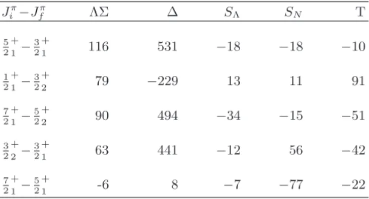
hyper-TABLE I. Contributions to energy-level spacings (in keV) from the components of the ΛN interaction. The corefficients of the parameters are determined by numerical differentia-tion. The contribution from Λ-Σ coupling is determined by diagonalizing with the coupling switched on and off. The dif-ference between the total contribution of 601 keV in the first line of the table and the 592 keV from diagonalization (see Fig. 1) is due to small differences in the sum of diagonal core energies caused by configuration mixing. Such differences are usually only a few tens of keV.

Jπ i −Jfπ ΛΣ ∆ SΛ SN T 5 2 + 1− 3 2 + 1 116 531 −18 −18 −10 1 2 + 1− 3 2 + 2 79 −229 13 11 91 7 2 + 1− 5 2 + 2 90 494 −34 −15 −51 3 2 + 2− 3 2 + 1 63 441 −12 56 −42 7 2 + 1− 5 2 + 1 -6 8 −7 −77 −22

TABLE II. The C2_{S values for proton removal from}9_{Be. The}

second through fourth columns contain the normalized exper-imental values, for the (d,3_{He) reactions (second and third}

columns) and normalized to the same summed strength (num-ber of p-shell protons in9_{Be) for the (t, α) reaction (fourth}

column). The values for one of the other interactions used in hypernuclear calculations are listed in the fifth column and the values from the Cohen and Kurath (6-16)2BME and the (8-16)2BME interactions [17] in the sixth and seventh columns. Jπ i [15] [16] [18] fit4 (6-16) (8-16) 2+ 1 1.00 1.03 0.78 1.00 1.00 0.95 1+ 1 0.42 0.39 0.47 0.45 0.40 0.20 3+ 1 0.33 0.30 0.51 0.36 0.35 0.33 1+2 0.04 0.06 0.24

nuclear studies are similar and in agreement with those for the Cohen and Kurath (6-16)2BME interaction [19]. The values for the other two Cohen and Kurath inter-actions put more strength in the second 1+ _{state than} in the first (as noted in Ref. [19] for the (8-16)POT in-teraction). The reason for this is that the 1+1 states are rather purely L = 1, S = 1, rather than with strongly mixed S = 0 and S = 1 components, as happens for the other interactions. Strength for the 1+

2 state would be immediately noticeable in electroproduction because the 9

ΛLi states based on the 1+2 state lie close to the neutron threshold at 3.73 MeV and should therefore be narrow.

The states in the first-excited doublet are predicted to be nearly degenerate, in part because of the

contribu-tions from Λ-Σ coupling (see Table I). In addition, the 3/2+2 state contains a 3.5% admixture of a Λ coupled to the8_{Li ground state which lowers the 3/2}+

2 state by an-other ≈ 35 keV. Thus, if the shell-model predictions are reasonable, five peaks should, in principle, be resolved in 9

ΛLi below the particle-decay threshold by an electropro-duction experiment with good energy resolution.

III. EXPERIMENT

Hall A at JLab is well suited to perform (e, e′_K+₎ ex-periments. Scattered electrons are detected in the High Resolution Spectrometer (HRS) electron arm while coin-cident kaons are detected in the HRS hadron arm [20]. The disadvantage of smaller electromagnetic cross sec-tions is compensated for by the high current and high duty cycle properties of the beam. Throughout the ex-periment, the same equipment has been used in very sim-ilar kinematical conditions on C, Be, and H2O targets. The use of a pair of septum magnets permitted particle detection at very forward angles [21] and a Ring Imag-ing CHerenkov (RICH) detector [22–25] has been used in the hadron arm to provide an unambiguous identifi-cation of kaons when combined with the standard parti-cle identification apparatus of Hall A, based on aerogel Cherenkov detectors [26–28]. In the present experiment a 92.5 mg/cm2 _solid 9_{Be target with a beam current of} ∼100 µA was used at a beam energy of 3775 MeV. Both HRSs were physically positioned at an angle of 12.5◦_{, but} the pair of septum magnets yielded an effective angle for both the scattered electron and the hadron detection of ∼ 6◦_.

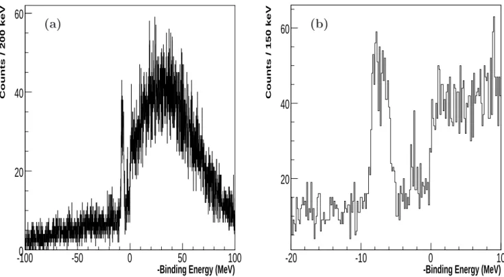
Fig. 2 shows the observed binding-energy spectrum of 9

ΛLi. The broad peak centered at a small positive bind-ing energy corresponds to the 9

ΛLi states in Fig. 1 cor-responding to the lowest three states of 8_{Li. The rise} in cross section starting at 0 MeV corresponds to states with the Λ in a p orbit and, because these states are unbound, the states are broad and no structure is ob-served. As in Ref. [4, 5], the background was determined from the binding energy spectrum obtained with a coin-cidence time shifted with respect to the coincoin-cidence time between secondary electrons and produced kaons and was rather flat for values of binding energy ranging from 15 MeV to 0 MeV. Its value was calculated as the average of the counts in the range 9.95 MeV ≤ Binding energy ≤ 18.35 MeV.

For the calculation of the absolute cross section, we computed the following quantities: detector efficiencies, detector dead time, detector phase space, kaon survival in HRS, integrated luminosity. The calculation of efficien-cies for the standard HRS package are well established and implemented in the Hall A analysis software. There-fore, those procedures were used for that purpose. For the RICH and aerogel Cherenkov detectors, we used one detector to determine the efficiency of the other one in the following way: we selected a pure sample of kaons

by means of aerogel detectors and we measured the frac-tion of those kaons detected by the RICH and vice versa. The detector dead time was measured by the Hall A data acquisition system. The detector phase space was lated using the SIMC code [29]. Kaon survival is calcu-lated considering the average path length inside the HRS arm. The integrated luminosity was calculated by means of beam current monitor devices. Then, the absolute cross section σ was computed according to

σ = Counts

Ksur · Ef f · Luminosity · P haseSpace · Livetime, (3) where Counts is the event number in the experiment, Ef f is the global detector efficiency, Livetime is 1-detector dead time, P haseSpace is the 1-detector phase space, Ksur is the kaon survival in the HRS, and Luminosity is the integrated luminosity.

Fig. 3 shows the background-subtracted experimen-tal binding-energy spectrum, together with Monte Carlo simulations[29] (red curve) and the same simulations with the radiative effects turned off (blue curve). The error bars in the data are statistical. The simulations used the five peak positions and widths listed as configuration α in Table IV. The red curve fits the experimental data well with a corresponding χ2_{/ndf value of 36.69/35.} Sev-eral other peak configurations, with different numbers, heights, positions and widths of the peaks, have been found to reproduce the red curve. All of those are also expected to generate the same spectrum (the blue curve of Fig. 3) when radiative corrections are turned off, since radiative corrections are independent of the assumptions regarding the number and type of the peaks that build up the experimental spectrum. In practice, the simulated data do not overlap perfectly with the experimental data, which produces small systematic errors on the radiatively corrected spectrum.

The unfolding for radiative corrections has been done bin-by-bin. The content of each bin of the radiatively corrected spectrum was obtained by multiplying the cor-responding bin of the experimental spectrum by the ratio of the blue and red curves of Fig. 3 for that bin. In order to avoid possible removals of background enhancements or to artificially null the spectrum in the regions where the blue curve is zero, the ratio between the blue and red curves of Fig. 3 was performed after summing the background to each of them. The background value was then subtracted from the result of the product of the ratio with the corresponding bin. The result is shown in Fig. 4 which presents the radiatively unfolded exper-imental data (points with statistical errors) compared to a theoretical prediction (thin green line). The band at the bottom of the histogram represents the system-atic errors in the radiative unfolding. The theoretical histogram was obtained using the procedure described in section II assuming an energy resolution of 730 keV (FWHM). Once radiative corrections have been applied, the binding-energy spectrum resolution is small enough to clearly show a three-peak structure in the spectrum.

-Binding Energy (MeV)

-100

-50

0

50

100

0

20

40

60

(a)

-Binding Energy (MeV)

-20

-10

0

10

Counts / 150 keV

20

40

60

(b)

FIG. 2. The binding-energy spectrum obtained after kaon selection with aerogel detectors and RICH in (a) the whole energy range and (b) restricted to the region of interest.

-Binding Energy (MeV)

-10 -9 -8 -7 -6 -5 -4 -3 GeV MeV)] 2 Cross Section [nb/(sr -0.2 0 0.2 0.4 0.6 0.8 1 1.2 1.4

FIG. 3. (Color online) The 9ΛLi differential cross section as

a function of the binding energy. Experimental points vs. Monte Carlo results (red curve) and vs. Monte Carlo results with radiative effects turned off (blue histogram).

A more detailed description of the procedure employed to determine the radiatively unfolded spectrum of Fig. 4 is given in Appendix A.

IV. RESULTS

When analyzing the experimental spectrum in Fig. 4 one has to consider that, as explained in section II, the

-Binding Energy (MeV)

-10 -9 -8 -7 -6 -5 -4 -3 -2 GeV MeV)] 2 Cross Section [nb/(sr -0.2 0 0.2 0.4 0.6 0.8 1 1.2 1.4

FIG. 4. (Color online) The radiatively unfolded experimental spectrum compared to a theoretical prediction (thin green line). The solid black line represents a fit to the data with four Gaussians of a common width. The theoretical curve was calculated with the width extracted from the fit (FWHM = 730 keV).

spectrum is made up by doublets and hence that each of the three peaks that appears in it is actually produced by the convolution of two “elementary” peaks. Because the peaks of the spectrum are radiatively corrected, we as-sumed that all the elementary peaks were well described by Gaussian distributions. Considering the energy res-olution to be constant over the whole spectrum range,

TABLE III. Excitation energies, widths, and cross sections obtained by fitting the 9_{Be(e, e}′_K+₎9

ΛLi spectrum (first three

columns), compared with theoretical predictions (last four columns). The last column gives the summed cross sections for the three doublets, to be compared with the experimental results in the third column.

Experimental data Theoretical predictions

Ex Width (FWHM) Cross section Ex Jπ Cross section Cross section

(MeV) (MeV) (nb/(sr2 _{GeV)) (MeV) (nb/(sr}2 _{GeV)) Sum}

0.00 ± 0.08 0.73 ± 0.06 0.59 ± 0.15 0.00 3/2+ _{0.18 1.22} 0.57 ± 0.12 0.73 ± 0.06 0.83 ± 0.13 0.59 5/2+ _1.04 1.47 ± 0.09 0.73 ± 0.06 0.79 ± 0.07 1.43 3/2+ _{0.29 0.59} 1.45 1/2+ _0.30 2.27 ± 0.09 0.73 ± 0.06 0.54 ± 0.06 2.27 5/2+ _{0.17 0.48} 2.74 7/2+ _0.31

we assumed in addition that the standard deviations of these Gaussians were equal. Although six Gaussian el-ementary peaks are expected, the possible existence of nearly degenerate doublets, or of doublets where one peak overwhelmingly dominates on the other, could re-duce the number of elementary Gaussian peaks needed for the fit procedure following the Occam razor principle. The experimental spectrum in Fig. 4 was fitted in order to determine the positions, the heights, and the common standard deviation of the elementary peaks. The best fit was obtained with four Gaussian elementary peaks with a χ2_{/n.d.f. value of 41.82/41. The energy} resolu-tion extracted from the fit, 730 keV (FWHM), is con-sistent with the value obtained in our previous analysis [30] and is in agreement with the measurements on12

ΛB [4] and16

ΛN [5]. The excitation energies (Ex) and cross sections extracted from the four-peak fit are reported in Table III where they are compared with the results cal-culated using the procedure described in section II for the six lowest states shown in Fig. 1. A fit with five Gaussian peaks produced the same result as shown in Table III with a χ2/ndf value of 41.82/39 and a common FWHM for the peaks of 730 keV. The first three peaks had the same heights and positions of the corresponding peaks in Table III while the fourth and fifth peaks had equal positions, coincident with the binding energy of the fourth peak in Table III and heights whose sum was equal to the cross section value of the fourth peak in Table III. The result of the five-peak fit showed hence that only the ground-state doublet splitting could be detectable with the energy resolution of the experiment. A fit with three peaks also produced a result consistent with Table III, with a χ2/ndf value of 47.52/43 and a common peak resolution extracted from the fit of 970 keV (FWHM). The first peak’s strength and position were equal (within one standard deviation) to the sum of the strengths and to the baricenter of the positions in the binding-energy spectrum of the first two states of Table III respectively. The other two peaks had strengths and positions equal (within one standard deviation) to the third and fourth

peaks in Table III respectively. Fig. 4 and Table III show that the observed peak positions agree quite well with the predictions of the standard model for p-shell hypernuclei. The first multiplet can be decomposed into two peaks with a separation of 570 ± 120 keV that cor-responds very well with the theoretical value of 590 keV. On the other hand, there is a systematic disagreement for the multiplet cross sections. In the first multiplet the 0.59 MeV (5/2+_{) peak does not dominate as theoretically} predicted (see Table III). The second and third multi-plets are each observed as a single peak. This is probably due to the very close excitation energies of their two con-stituents (see Table III), although for the third multiplet it might be due to the fact that the strength of the 2.27 MeV (5/2+_{) peak dominates over that of the other state.} In terms of the cross section, the spin-spin interaction (∆) tends to deplete the spin-flip strength to the ground-state doublet and increase the non-spin-flip strength (see Fig. 1). The full reaction calculations include a number of spin-flip and non-spin-flip amplitudes, making the cross sections sensitive to the choice of the elementary reaction model. The SLA model was selected from the various iso-bar models because it gives the best results for the cross section. Spin-flip amplitudes are dominant in the SLA model which favors states in Fig. 1 with large ∆S = 1 structure amplitudes. It is then clear that a model with larger non-spin-flip amplitudes might increase the rela-tive cross sections for the 3/2+1 and 5/2+2 states and pro-vide better agreement with the results of the experimen-tal analysis. The cross section depends very much on the proton removal spectroscopic factors for9_{Be but, as} is evident from Table II, theory agrees very well with the relative C2_{S values derived from the analysis of two} (d,3_{He) studies, a reaction that has proven to be very} reliable for such a comparison.

From the binding-energy spectrum of Fig. 4, a Λ sepa-ration energy BΛ of 8.36 ± 0.08 (stat.) ± 0.08 (syst.) MeV was obtained. This value agrees very well with the value 8.50 ± 0.12 MeV from emulsion data [33]. To determine this value the missing-mass scale needed to

be calibrated because of uncertainties in the kinemat-ical variables such as the primary electron energy and the central momenta and the central scattering angles of the scattered electrons and the produced kaons. For this calibration we took advantage of the fact that the ex-periment was performed just after the determination of the 12

ΛB excitation spectrum [4] that used the same ex-perimental settings. Thus, the kinematical variables of the present experiment were determined, reproducing the binding energy of the 12

ΛB ground state at 11.37 ± 0.06 MeV [33]. A more detailed description of this missing-mass scale calibration is given in Appendix B.

V. SUMMARY

A high-quality9

ΛLi hypernuclear spectrum has been ob-tained for the first time with sub-MeV energy resolution. The measured cross sections and the excitation energies of the doublets are in a good agreement with the values predicted using the SLA model and simple shell-model wave functions while a disagreement could exist with re-spect to the relative strengths of the states making up the first multiplet. As noted in the Sec. IV, an elementary model for the (e, e′_K+_{) reaction with a different balance} of spin-flip and non-spin-flip amplitudes might help to resolve this disagreement. A Λ separation energy BΛ of 8.36 ± 0.08 (stat.) ± 0.08 (syst.) MeV was obtained, in good agreement with the emulsion value.

Appendix A: Radiative corrections

The procedure of unfolding radiative effects from an experimental spectrum does not depend on the choice of the peak structure used to fit the spectrum itself, provid-ing that the fit describes the data reasonably. This prop-erty is very useful when the peak structure underlying an experimental spectrum is unknown as in Fig. 3, where several peak structures fit the experimental spectrum quite well and it is not obvious which of these structures is “the right one”. To demonstrate the independence of radiative corrections from the energy spectrum struc-ture, we define Exp(E) as the function that describes the experimental spectrum. Exp(E) · dE is proportional to the number of events whose corresponding energy is in the interval E ± dE. We define S(E′_{) as the function} that describes the experimental spectrum in the absence of radiative effects. Lastly, we define R(E′ _{− E) as the} probability that an event whose corresponding energy in the absence of radiative effects would have been E′ _has, because of the radiative effects, an energy equal to E. Exp(E), S(E′_{) and R(E − E}′_{) are related by}

Exp(E) · dE = dE · Z

dE′_{· R(E}′_{− E) · S(E}′_{) (A1)}

For the sake of simplicity, we suppose in the following that S(E′_{) is equal to a sum of Gaussian peaks}

S(E′_{) =} N X k=1 Ak· e −(E′ −Ek) 2 2·σ2_{k , (A2)}

where Ak, Ek and σk are the amplitude, central value and standard deviation of the kth peak, respectively.

Let us assume two different peak configurations α and β, with N and M peaks, respectively, that produce two functions Sα_(E′_{) and S}β_(E′_{) that are equal within the} statistical error Sα_(E′_{) =} N X k=1 Ake −(E′ −Ek) 2 2·σ2_{k ≈} M X l=1 Ale −(E′ −El) 2 2·σ2_{l = S}β_(E′₎ (A3) This implies that for every value of E′_{, S}α_(E′_{) and} Sβ_(E′_{) have statistically compatible values and the χ}2 test χ2=X j (Sα j − S β j)2 Sα j , (A4) with S_jα,β = Z Ej′ E′ j−1 dE′_{· S}α,β_(E′_{) , (A5)}

is acceptable within our confidence level. In Eq. (A5), [Ej−1; Ej] is the jth interval that the energy spectrum is divided into.

It is obvious from Eq. (A1) that if Sα_(E′_{) = S}β_(E′_{) the} two peak configurations α and β will produce the same experimental spectrum, that is Expα_{(E) = Exp}β_(E).

The reverse is also true: if two peak configurations α and β produce two statistically compatible spectra (Expα_{(E) = Exp}β_{(E)) then S}α_(E′_{) = S}β_(E′_{). In fact,} defining Expi= Z Ei Ei−1 dE · Exp(E) , (A6) and Rij = Z Ei Ei−1 dE · R(E′_{− E) , (E}′ _{∈ [E}′ j−1; Ej′]) (A7) we have from Eq. (A1)

Z Ei Ei−1 dE · Exp(E) = Z dE′_{· S(E}′₎ Z Ei Ei−1 dE · R(E′_{− E)} (A8) Eq. (A8) means that

Expi= X

j

Excitation Energy (MeV) 0 2 4 6 8 10 12 0 200 400 600 800 1000 1200 1400 1600 1800 2000 2200

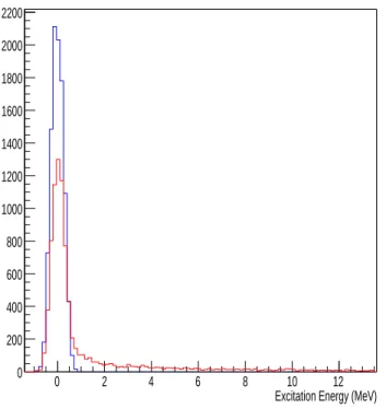
FIG. 5. (Color online) One peak of the excitation energy spectrum of the hypernucleus9

ΛLi obtained through the

reac-tion9_{Be(e, e}′_K+₎9

ΛLi as predicted by the Monte Carlo SIMC

when including all effects (red curve) and “turning off” the radiative effects (blue curve). Arbitrary units. The position of the peak has been made coincident with the ground state.

or, defining the arrays−−→Exp ≡ {Exp1, Exp2, ...Expi, ...} and −→S ≡ {S1, S2, ...Sj, ...}, and the matrix R ≡ {R11, R12, ..., Rij, ...}

−−→

Exp = R ·−→S (A10)

Defining at last R−1 _{as the inverse of the matrix R, we} have

− →

S = R−1_·−−→_{Exp (A11)} From Eq. (A11) it follows that if Expα_{(E) = Exp}β_(E) then Sα_(E′_{) = S}β_(E′_{). In fact,}

Expα= Expβ⇒ 0 = R−1_{· (}−−−→_Expα₋−−−→_Expβ₎ =−S→α₋−_S→β_{⇒ S}α_{= S}β _(A12) means that the spectrum with the radiative effects sub-tracted (S(E′_{)) does not depend on the peak} configura-tions α, β, · · · as long as all the configuraconfigura-tions considered Expα_{, Exp}β_{, · · · fit the experimental spectrum with no} radiative effects applied. It has to be noted that only two assumptions were made in deriving the conclusion quoted above

• the single intervals [Ej−1; Ej] are so small that Rij defined by Eq. (A7) is constant in it.

• The matrix R is invertible. This is usually the case considering that usually Rii 6= 0 and Rji = 0 if Rij6= 0 and i 6= j

TABLE IV. Columns 2 and 3: peak positions and relative amplitudes of five configurations α, β, γ, δ and ǫ for which the Monte Carlo SIMC predicts a9

ΛLi excitation energy spectrum

that fits the experimental data. Column 4: the χ2_{test values}

calculated through Eq. (A13) for these configurations. Configuration Peak Positions Peak Amplitudes χ2

MeV Arbitrary units 35 ndf

0.00 2.23 0.64 3.54 α 1.32 1.90 36.685 1.71 2.61 2.35 2.33 0.00 2.08 0.58 3.48 β 1.54 3.38 38.247 2.37 2.10 0.00 2.34 0.54 3.88 γ 1.49 3.78 46.088 2.36 3.28 0.00 1.86 0.54 3.08 δ 1.49 3.00 39.068 2.36 2.06 0.00 1.85 0.65 3.09 ǫ 1.43 3.00 39.000 2.39 2.06

To determine the spectrum with the radiative effects “turned off” (blue curve of Fig. 3) the Monte Carlo SIMC was employed [29]. The red curve of Fig. 5 shows a single peak of the9

ΛLi excitation energy spectrum as predicted by SIMC for the reaction 9_{Be(e, e}′_K+₎9

ΛLi when using the E94-107 experimental apparatus (position and am-plitude of the peak are arbitrary). The blue curve of Fig. 5 shows the same peak when the radiative effects in the Monte Carlo SIMC are “turned off”. Several peak configurations, made up by a number of peaks like the one of Fig. 5 red curve, fit the experimental9

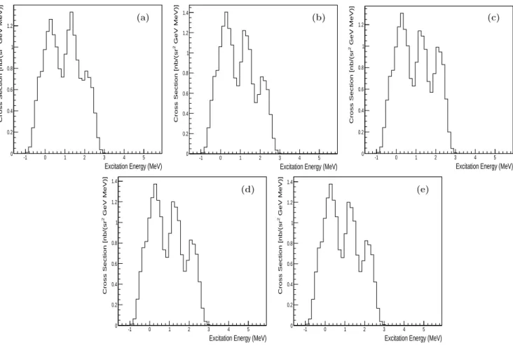
ΛLi excitation energy spectrum after being normalized to it. Table IV quotes five of them. Their corresponding excitation en-ergy spectra (normalized to the experimental data) are shown in Fig 6. For each configuration, Table IV quotes the position and relative amplitude of the peaks (here and in the following the amplitude of a peak is defined as the integral of the peak over the whole energy spectrum) and the value of the χ2 _test,

χ2=X i

(C_iconf− Expi)2 Expi

, (A13)

where conf = α, β, γ, δ, or ǫ, Expi is the number of counts in the ith interval of the experimental excitation energy spectrum, and C_iconf is the number of counts in the same interval as predicted by the normalized peak

Excitation Energy (MeV) -1 0 1 2 3 4 5 GeV MeV)] 2 Cross Section [nb/(sr 0 0.1 0.2 0.3 0.4 0.5 0.6 0.7 0.8 (a)

Excitation Energy (MeV)

-1 0 1 2 3 4 5 GeV MeV)] 2 Cross Section [nb/(sr 0 0.1 0.2 0.3 0.4 0.5 0.6 0.7 0.8 (b)

Excitation Energy (MeV)

-1 0 1 2 3 4 5 GeV MeV)] 2 Cross Section [nb/(sr 0 0.1 0.2 0.3 0.4 0.5 0.6 0.7 0.8 (c)

Excitation Energy (MeV)

-1 0 1 2 3 4 5 GeV MeV)] 2 Cross Section [nb/(sr 0 0.1 0.2 0.3 0.4 0.5 0.6 0.7 0.8 _(d)

Excitation Energy (MeV)

-1 0 1 2 3 4 5 GeV MeV)] 2 Cross Section [nb/(sr 0 0.1 0.2 0.3 0.4 0.5 0.6 0.7 0.8 (e) FIG. 6. 9

ΛLi excitation energy spectra as predicted by the Monte Carlo SIMC for the peak configurations α, β, γ, δ and ǫ

quoted in Table IV (Panels (a), (b), (c), (d) and (e), respectively).

configuration conf . The χ2 _{tests were performed in the} interval -1.515 MeV < Excitation Energy < 3.735 MeV, corresponding to 35 degrees of freedom.

Because of the properties of the subtraction of radia-tive effects from spectra quoted above, all the peak con-figurations α, β, γ, δ, and ǫ produce the same “radiatively corrected” spectrum. The spectra of Fig. 7 are obtained from Fig. 6 by turning off the radiative effects, that is replacing the “Fig. 5 red curve-like” peaks with “Fig. 5 blue curve-like” peaks, without changing positions and amplitudes of the peaks. All plots of Fig. 7 are quite equal, as confirmed by the χ2_test,

χ2=X i (Cconf1 i − C conf2 i )2 Cconf1 i , (A14)

with conf1and conf2= α, β, γ, δ, or ǫ. In the worst case (conf1= α and conf2= γ) Eq. (A14) yielded a value of 28.387 with 40 degrees of freedom.

In Fig. 8(a), Fig. 7(a) (dashed line) and Fig. 7(c) (con-tinuous line) are shown together. Because the configura-tions α and γ produce the two most different “radiatively corrected” SIMC results, the difference between the two curves plotted in Fig. 8(a) was chosen as the systematic

error due to the ambiguity of the peak structure under-lying the energy spectrum. As shown in Fig. 8(b) this error is small compared to the statistical error.

The method to obtain radiative corrected spectra de-scribed in this Appendix was used, in the analysis of the 9

ΛLi spectrum, because of the difficulties in estab-lishing the peak structure underlying the experimental spectrum. It is relatively new and it could be worth-while hence to make some considerations about its reli-ability. The method relies on Eq. (A11) that is math-ematically correct. The uncertainties on the radiative corrected spectrum−→S derived by Eq. (A11) originate ob-viously from the uncertainties on the experimental spec-trum−−→Exp and on the function R−1 _{(”detector function”} in the following) that provides −→S once −−→Exp has been measured. If−−→Exp and R−1 _{were exempt from errors}−→_S would be ”perfect”. To understand the effects on the reconstructed radiative spectrum of the uncertainties on the measured spectrum and on the detector function it could be worthwhile to look at the results of the method to derive a neutron energy spectrum from the proton re-coil energy measurement (see for example [31, 32]). This method consists in determining a neutron energy

spec-Excitation Energy (MeV) -1 0 1 2 3 4 5 GeV MeV)] 2 Cross Section [nb/(sr 0 0.2 0.4 0.6 0.8 1 1.2 (a)

Excitation Energy (MeV)

-1 0 1 2 3 4 5 GeV MeV)] 2 Cross Section [nb/(sr 0 0.2 0.4 0.6 0.8 1 1.2 1.4 (b)

Excitation Energy (MeV)

-1 0 1 2 3 4 5 GeV MeV)] 2 Cross Section [nb/(sr 0 0.2 0.4 0.6 0.8 1 1.2 (c)

Excitation Energy (MeV)

-1 0 1 2 3 4 5 GeV MeV)] 2 Cross Section [nb/(sr 0 0.2 0.4 0.6 0.8 1 1.2 1.4 (d)

Excitation Energy (MeV)

-1 0 1 2 3 4 5 GeV MeV)] 2 Cross Section [nb/(sr 0 0.2 0.4 0.6 0.8 1 1.2 1.4 (e) FIG. 7. 9

ΛLi excitation energy spectra as predicted by the Monte Carlo SIMC for the peak configurations α, β, γ, δ and ǫ

quoted in Table IV, when the radiative effects are “turned off” (Panels (a), (b), (c), (d) and (e), respectively).

Excitation Energy (MeV)

-1 0 1 2 3 4 5 GeV MeV)] 2 Cross Section [nb/(sr 0 0.2 0.4 0.6 0.8 1 1.2 (a)

Excitation Energy (MeV)

-2 -1 0 1 2 3 4 5 6 GeV MeV)] 2 Cross Section [nb/(sr -0.2 0 0.2 0.4 0.6 0.8 1 1.2 1.4 _(b)

FIG. 8. (a) the spectrum of the configuration α (dashed line) and of the configutration γ (continuous line) as predicted by the Monte Carlo SIMC when the radiative effects are “turned off”. (b) the statistical errors (error bars) and the systematic errors (full band) as a function of the excitation energy. The systematic error was defined as the difference between the dashed line and the continuous line of panel (a), see text for details.

trum measuring the energies of the protons generated by scatterings of the neutrons in a radiator and is for-mally similar to the one described in this Appendix to derive radiative corrected spectra from the experimen-tal ones. Formally, the connection between the neutron energy spectrum and the proton recoil energy spectrum can be expressed by a formula like Eq. (1) quoted in Ref. [31] that can be concisely expressed as:

F (En)dEn= D−1· Y (Ep)dEp. (A15) Here F (En)dEn is the number of neutrons in the neu-tron spectrum with an energy included in the interval En− dEn < En < En+ dEn, Y (Ep)dEp is the number of protons in the experimental spectrum with an energy Ep− dEp < Ep < Ep + dEp, and D−1 is the ”detec-tor function”. Defining −→N and −→P the arrays whose el-ements are F (En)dEn and Y (Ep)dEp respectively (En and EP covering the whole neutron and proton spectra), Eq. (A15) transforms into:

− →

N = D−1_·−→_{P . (A16)} Eq. (A16) is formally equivalent to Eq. (A11) (in Eq. (A16) D−1 _{is a diagonal matrix).}

However, in Eq. (A16) the knowledge on−→P is (some-times greatly) affected by the uncertainties on the mea-sured recoil proton energy. These uncertainties mean that the determination of the number of protons YpdEp whose real energy is included in the ith interval of the proton energy spectrum−→P and hence the proton energy spectrum itself are affected by (sometimes not negligi-ble) uncertainties too. Several factors affect the proton energy measurement: detector calibration, background subtraction, and, above all, proton energy losses in the detector elements (including their entrance windows) and in the air between them. To correct for proton energy losses, the proton energies are shifted by the estimated average energy loss over possible proton paths, or, some-times, in low energy regions, by unfolding techniques. The proton energy losses set usually the low limit of the reconstructed neutron energy spectrum. The detector function D−1 _{in Eq. (A16) is affected by uncertainties} too. It includes the detector efficiency that depends on the geometry (and on the connected problem of the de-termination of the scattering angle of the detected pro-ton) and on the differential n - p scattering cross section which are both sources of systematic errors. The differ-ential n - p scattering cross section is often obtained by parameterizations. Despite these problems, the method to derive a neutron energy spectrum from the proton re-coil energy measurement provides usually satisfactorily results. In Ref [31], the method was applied to deter-mine the spectra of nearly monoenergetic neutrons form the reaction7_Li(p,n)7_{Be measured for eight incident} pro-ton energies. The situation was here complicated by the

fact that, together with the neutrons generated in the re-action under study, which corresponded to a well-defined peak in the neutron energy spectrum, the experiment detected neutrons by other reactions, as the three-body breakup process7_Li(p,n3_{He)α, that generated a long tail} in the low energy region of the neutron energy spectrum. Despite that, the reproduction of the peaks of the eight neutron energy spectra was excellent, while the neutron counts in the tails of these spectra was somehow big-ger than the corresponding parts of the spectra obtained with a Time Of Flight (TOF) detector for three of the eight incident proton energies. The authors decided to rely on the TOF detector results for the tails of these three spectra because the TOF detector was free from the problems concerning the effects of the proton energy loss by reactions in the detectors and becuase it extended to lower energies than the method based on the proton recoil energy measurement. In Ref. [32] the situation was improved with respect to Ref. [31] because the de-tector function D−1 _{was simply equal, for all the proton} energies, to 1

cos2_(θ), with θ, the proton scattering angle,

measured by two silicon strip detectors for the most ener-getic protons and, less precisely, through the coordinates of the conversion point of the neutron inside the con-verter and the coordinates of the silicon detector closer to the converter for the protons whose energies were not big enough to make them reach the other silicon strip detector. The use of a segmented converter decreased the uncertainties on the proton energies due to energy losses inside the converter itself. As a consequence, the minimum neutron energy detectable was lower than the one of Ref. [31]. The double differential neutron yield for the reaction13_{C(d,n) at 40 MeV was obtained this} way. The good successes obtained in determining neu-tron spectra from the measurements of the proton recoil energies and the understanding of the effects that could make this method less effective ensure that we can rely on the method described in this Appendix to obtain, in the experiments performed at JLab, radiative corrected spectra from experimental binding energy spectra of hy-pernuclei. In fact, in these experiments, the hypernuclei are generated in point-like targets and the experimental binding energy spectra are obtained by the measurements of the momenta and the scattering coordinates of the sec-ondary electrons and of the produced kaons in the reac-tion Z(e, e′_K+_{)Z − 1. These momenta and scattering} coordinates are determined very precisely by magnetic spectrometers (at the level of 10−4_{for the momenta} mea-sured by HRS arms). The energy losses of the secondary electrons and of the produced kaons inside the target and along the path to the detectors are small. Moreover, thanks to the excellent Particle Identification apparatus employed, the experimental spectrum of the experiment E94-107 was pratically background free, the only small background coming from kaons from accidental coinci-dences. The uncertanties on−−→Exp of Eq. (A11) are hence much smaller than the uncertanties on−→P of Eq. (A16). Besides, the uncertainties on the detector function R−1

in Eq. (A11) are smaller than the uncertainties on the corresponding function D−1 _{in Eq. (A16) because of the} simpler geometries involved, the smaller uncertainties on the scattering angles of the detected particles and of the QED cross sections involved in the function R−1 _better known than the neutron - proton cross sections involved in the function D−1_.

Appendix B: Missing-mass scale

In the Hall A experimental setup, scattered electrons and produced kaons of the reactions 9_{Be(e, e}′_K+₎9

ΛLi and 12_{C(e, e}′_K+₎12

ΛB were detected by the High Res-olution Spectrometer (HRS) electron arm and by the HRS hadron arm, respectively, while the primary elec-trons were provided by the CEBAF accelerator. The CEBAF accelerator electron beam energy and the cen-tral momenta and angles of the HRS electron and hadron arms were set according to the kinematics of the reactions and are taken as constant for the course of the experi-ment (their variations being of the order of 10−5 _{for the} CEBAF electron beam energy and the central momenta of the HRS electron and hadron arms, and practically zero for the spectrometer central angles). However, the actual values of the CEBAF accelerator electron beam energy and of the central momenta and angles of the HRS electron and hadron arms, although constant, differ by unknown amounts from the nominal set values, and are referred to as “kinematical uncertainties”. Although small (the experimental uncertainties on the CEBAF ac-celerator electron beam energy and on the spectrometer central momenta being of the order of 10−4 _{- 10}−3 _and those on the spectrometer central angles of the order of 10−2_{), these kinematical uncertainties cause a global shift} in the binding-energy spectrum that hence has to be cal-ibrated. In fact, the binding energy is expressed as

Ebind= −p(Em)2− (Pm)2+ Mresidue+ MΛ , (B1) with

Em= MT arget+ Ee− Ee′− EK, (B2)

and

~

Pm= ~Pe− ~Pe′− ~PK , (B3) where Ee, ~Pe, Ee′, ~P_e′, E_K, and ~P_K are the energies and

the momenta of the primary electron, of the scattered electron and of the produced kaon respectively, MΛis the Λ mass, MT arget is the target mass, and Mresidue is the mass of the residual nucleus, that is of the nucleus with A-1 nucleons and Z-1 protons (where A is the number of nucleons and Z is the atomic number of the target, respectively).

The change in the binding-energy spectrum ∆Ebind caused by the kinematical uncertainties can be expressed

by the formula ∆Ebind= ∂Ebind ∂Ee · ∆Ee+ ∂Ebind ∂PE Arm · ∆PE Arm + ∂Ebind ∂PH Arm · ∆PH Arm+ ∂Ebind ∂φE Arm · ∆φE Arm + ∂Ebind ∂φH Arm · ∆φH Arm, (B4)

where Ee is the CEBAF electron beam energy, PE Arm and PH Arm are the central momenta of HRS electron arm and HRS hadron arm, φE Arm and φH Arm are the central angles (defined as the angles between the central axes and the CEBAF beam line) of HRS electron arm and HRS hadron arm, and ∆Ee, ∆PE Arm, ∆PH Arm,

∆φE Arm and ∆φH Arm are the kinematical

uncertain-ties, that is the differences between the nominal and the actual values of the CEBAF electron beam energy and of the central momenta and the central angles of HRS elec-tron and HRS hadron arms. ~Pe, Ee′, ~P_e′, E_K, and ~P_K

in Eq. (B1) - (B3) are functions of Ee, PE Arm, PH Arm, φE Armand φH Arm, as well as (with the exception of ~Pe) of the scattering variables. For example, the components normal to the beam line in the horizontal plane of ~Pe′and

~

PK respectively (called here Pe′

x and PKx, respectively)

are given by the expressions Pe′

x = PE Arm· (1 + δe′) ·

cos(θe′) · sin(φ_{E Arm}+ φ_e′) and P_Kx = P_{H Arm}· (1 + δ_K) ·

cos(θK)·sin(φH Arm+ φK), while Ee′ = P_{E Arm}·(1 + δ_e′)

and EK =p(PH Arm· (1 + δK))2+ m2k, where δe′ (δK) is the percentage difference between the momentum of the scattered electron (produced kaon) and the central momentum of the HRS electron arm (HRS hadron arm), φe′ (φ_K) is the angle between the electron (produced

kaon) direction in the horizontal plane, and φE Arm (φH Arm), θe′ (θK) are the angles between the electron (produced kaon) direction in the vertical plane and the CEBAF beam line, and mK is the kaon mass.

Considering Eqs. (B1), (B2), and (B3), Eq. (B4) is equal to

∆Ebind= (−∆Ee+ ∆PE Arm+ ∆PH Arm)

×q MT arget+ Ee− Ee′− EK (MT arget+ Ee− Ee′− E_K)2− ( ~P_e− ~P_e′− ~P_K)2 + f 2 · q (MT arget+ Ee− Ee′− E_K)2− ( ~P_e− ~P_e′− ~P_K)2 (B5) where f =∂( ~Pm) 2 ∂Ee · ∆Ee+ ∂( ~Pm)2 ∂PE Arm · ∆PE Arm + ∂( ~Pm) 2 ∂PH Arm · ∆PH Arm+ ∂( ~Pm)2 ∂φE Arm · ∆φE Arm + ∂( ~Pm) 2 ∂φH Arm · ∆φH Arm (B6)

For the kinematics of the experiment E94-107 (see the nominal values of Ee, Ee′, and E_K at the end of this

Ap-pendix) or if MTarget ≫ Ee, Ee′, EK, the change in the binding-energy spectrum ∆Ebindcaused by the kinemat-ical uncertainties is

∆Ebind∼ S + T , (B7)

where

S = −∆Ee+ ∆PE Arm+ ∆PH Arm, (B8) and

T = M−1 Target·

f

2 . (B9)

The term S does not depend on the target mass and causes a global shift of the binding-energy spectrum without changing the peak shapes and relative posi-tions, while the term T is equal to zero only when 0 = ∆Ee= ∆PE Arm= ∆PH Arm= ∆φE Arm= ∆φH Arm. When this condition is not fulfilled, the main effect of T on the binding-energy spectrum is to broaden the peaks because, in this case, depending on scattering variables through ~Pm, it produces non-zero, scattering variable de-pendent values of ∆Ebind and, as a consequence, an un-physical dependence on the scattering variables of the binding energy that broadens the peaks corresponding to the bound states. Because of the presence of the co-efficient M−1

Target, the effect of T on the position of the peaks is negligibly small.

The actual values of Ee, PE Arm, PH Arm, φE Arm, and φH Arm are hence those for which S = T = 0 (which places a peak at its known position in the binding energy spectrum and minimizes its FWHM).

To determine the Λ binding energy of the hypernucleus 9

ΛLi produced in the reaction 9Be(e, e′K+)9ΛLi, we took advantage of the fact that the experiment used the same set-up employed for the study of the12

ΛB hypernucleus. The values of Ee, PE Arm, PH Arm, φE Arm, and φH Arm were thus the same in the productions of both 9

ΛLi and 12

ΛB and were determined by positioning the12ΛB ground state at its known position of 11.37 ± 0.06 MeV [33] in the binding-energy spectrum and minimizing its FWHM. When minimizing the12

ΛB ground-state FWHM, it has to be taken into account that this ground state is actually a doublet whose energy splitting, assumed to be equal to the12

ΛC ground-state energy splitting, is 161.6 ± 0.2 keV [34, 35]. Minimizing the 12ΛB ground-state FWHM implies hence some sort of distortion because it artifi-cially narrows the positions of the peaks making up the doublet. However, the 12

ΛB ground-state doublet energy splitting is small enough with respect to the energy res-olution of the experiment to make the approximation of assuming the12ΛB ground state as a single peak still valid. No attempt to minimize the FWHM was performed on the other peaks of the12

ΛB binding-energy spectrum. An-other possibile source of distortion comes from the term

T in Eq. (B7), which, although small because of the pres-ence of the factor M−1

T arget in it (see Eq. (B9)), can po-tentially change the positions of the excited states with respect to each other and with respect to the ground state. During all the process of minimization of the kine-matical uncertainties, the positions of the peaks of the 12

ΛB energy spectrum as resulted by a fitting procedure were checked to ensure that the relative peak positions did not change within the errors (the error of a position peak being defined as the standard deviation resulting by the fitting procedure). It has to be stressed that the term S in the expression of ∆Ebind given by Eq. (B7) dominates because of the presence of the factor M−1

T arget in the term T (see Eq. (B9)). The positioning of the 12

ΛB ground state at its known value in the binding spec-trum was thus mainly performed choosing a set of values

∆Ee, ∆PE Arm, and ∆PH Arm that produced a value of

S equal to the difference between the measured and the expected position of the 12

ΛB ground state. The mini-mization of the12

ΛB ground state peak FWHM produces only second order effects on the position of the peaks in the binding-energy spectrum and was peformed mainly to choose the right set of values ∆Ee, ∆PE Arm, and

∆PH Arm among the ∞2 sets of values that produced

the desired value of S. Things are much different for the reaction p(e, e′_K+_{)Λ, where the target mass is small and} the minimization of the FWHM of the peak (which is a single peak) plays a role as important as the positioning of the peak in the binding-energy spectrum to its zero value.

The procedure described above resulted in the set of values Ee = 3775.38 MeV, PE Arm = 1573.63 MeV,

PH Arm = 1955.79 MeV, φE Arm = −5.940◦, and

φH Arm= 6.050◦. Replacing with these values the

nom-inal ones Ee = 3774.96 MeV, PE Arm = 1570 MeV,

PH Arm= 1960 MeV, φE Arm= −5.873◦, and φH Arm=

6.131◦_{) in the E}

bind expression, a value of 8.36 ± 0.08 (stat.) MeV was obtained for the9

ΛLi ground state. The statistical error of ±0.08 MeV is the error in the position of the first peak in the four-Gaussian fit of the 9

ΛLi binding-energy spectrum (see Fig. 4 and Table III). When evaluating the systematic error of the 9

ΛLi bind-ing energy, one has to consider that, as quoted above, the term S in ∆Ebind dominates the effects of the term T . When neglecting the energy loss in the target, this means that if the single values of ∆Ee, ∆PE Arm, and

∆PH Armwere wrong, the9ΛLi binding energy would not

be affected significantly as long as the sum S (and hence the position of the12ΛB ground state) is correctly repro-duced. The major source of systematic error is hence due to the energy loss in the target. The difference between the shifts of the ground-state position in the 12

ΛB and 9

ΛLi binding-energy spectra due to the energy loss in the targets of12_{C and}9_{Be, respectively, was evaluated to be} equal to 50 keV through the use of the Monte Carlo code SIMC [29]. This value was added in quadrature to the error of 60 keV quoted for the12

ΛB ground-state binding energy [33] to give a 80 keV systematic error on the9

binding energy.

ACKNOWLEDGMENTS

We want to remember F. Cusanno, who enthusiasti-cally and greatly contributed to this paper before his un-timely death. We acknowledge the Jefferson Lab Physics and Accelerator Division staff for the outstanding

ef-forts that made this work possible. This material is based upon work supported by the Department of En-ergy, Office of Energy Research, under contract DE-AC05-06OR23177, by the Italian Istituto Nazionale di Fisica Nucleare, by the Grant Agency of the Czech Re-public under grant No. P203/12/2126, by the French CEA and CNRS/IN2P3, and by the U.S. National Sci-ence Foundation.

[1] O. Hashimoto and H. Tamura, Prog. Part. Nucl. Phys. 57, 564 (2006).

[2] H. Tamura et al., Nucl. Phys. A 804, 73 (2008). [3] T. Motoba, P. Bydzovsky, M. Sotona, and K. Itonaga,

Prog. Theor. Phys. Suppl. 185, 224 (2010).

[4] M. Iodice et al., Phys. Rev. Lett. 99, 052501 (2007). [5] F. Cusanno et al., Phys. Rev. Lett. 103 202501 (2009). [6] T. Miyoshi et al., Phys. Rev. Lett. 90, 232502 (2003); [7] L. Yuan et al., Phys. Rev. C 73, 044607 (2006); [8] S.N. Nakamura et al., Phys. Rev. Lett. 110, 012502

(2013).

[9] F. Garibaldi, S. Frullani, P. Markowitz and J. LeRose, spokespersons, JLab Experiment E94-107, High Resolu-tion 1p shell Hypernuclear Spectroscopy (1994). [10] M. Sotona and S. Frullani, Prog. Theor. Phys. Suppl.

117, 151 (1994).

[11] D. J. Millener, Nucl. Phys. A 804, 84 (2008). [12] D. J. Millener, Nucl. Phys. A 881, 298 (2012).

[13] T. Mizutani, C. Fayard, G.-H. Lamot and B. Saghai, Phys. Rev. C 58, 75 (1998).

[14] D. J. Millener, in Topics in Strangeness Nuclear Physics, Lecture Notes in Physics, Vol. 724, edited by P. Bydˇzovsk´y, A.Gal, and J. Mares (Springer, New York, 2007), p. 31.

[15] U. Schwinn, G. Mairle, G. J. Wagner and Ch. R¨amer, Z. Phys. A 275, 241 (1975).

[16] M. A. Oothoudt and G. T. Garvey, Nucl. Phys. A 284, 41 (1977).

[17] S. Cohen and D. Kurath, Nucl. Phys. 73, 1 (1965). [18] G.-B. Liu and H. T. Fortune, Phys. Rev. C 38, 1985

(1988).

[19] S. Cohen and D. Kurath, Nucl. Phys. A 101, 1 (1967). [20] J. Alcorn et al., Nucl. Instrum. Methods Phys. Res., Sect.

A 522, 294 (2004).

[21] G. M. Urciuoli et al., Nucl. Phys. A 691, 43c (2001). [22] M. Iodice et al., Nucl. Instrum. Methods Phys. Res., Sect.

A 553, 231 (2005).

[23] F. Garibaldi et al., Nucl. Instrum. Methods Phys. Res., Sect. A 502, 117 (2003).

[24] F. Cusanno et al., Nucl. Instrum. Methods Phys. Res., Sect. A 502, 251 (2003).

[25] G. M. Urciuoli et al., Nucl. Instrum. Methods Phys. Res., Sect. A 612, 56 (2009).

[26] R. Perrino et al., Nucl. Instrum. Methods Phys. Res., Sect. A 457, 571 (2001).

[27] L. Lagamba et al., Nucl. Instrum. Methods Phys. Res., Sect. A 471, 325 (2001).

[28] S. Marrone et al., Nuovo Cimento B 124, 99 (2009). [29] R. Ent et al., Phys. Rev. C 64, 054610 (2001);

https://hallcweb.jlab.org/wiki/index.php/Monte Carlo. [30] F. Cusanno et al., Nucl. Phys. A 835, 129 (2010); F.

Garibaldi et al., Nucl. Phys. A 914, 34 (2013).

[31] M. Baba et al., Nucl. Instrum. Methods Phys. Res., Sect. A 428, 454 (1999).

[32] A. Donzella et al., Nucl. Instrum. Methods Phys. Res., Sect. A 613 , 58 (2010).

[33] M. Juri´c et al., Nucl. Phys. B 52, 1 (1973). [34] Y. Ma et al., Nucl. Phys. A 835, 422 (2010). [35] K. Hosomi et al., Nucl. Phys. A 914, 184 (2013).