Arterial blood pressure estimation using ultrasound technology and transmission line arterial model

(1)

Arterial Blood Pressure Estimation using Ultrasound Technology and Transmission Line Arterial Model

by Kyle A. Beeks

S.B. in Electrical Engineering and Physics Massachusetts Institute of Technology (2017)

Submitted to the Department of Electrical Engineering and Computer Science in Partial Fulfillment of the Requirements for the Degree of

Master of Engineering in Electrical Engineering and Computer Science at the

Massachusetts Institute of Technology February 2019

c

The author hereby grants to M.I.T. permission to reproduce and to distribute publicly paper and electronic copies of this thesis document in whole and in part in any

medium now known or hereafter created.

Author:

Department of Electrical Engineering and Computer Science February 1, 2019

Certified by:

Charles G. Sodini

LeBel Professor of Electrical Engineering Thesis Supervisor

February 1, 2019

Accepted by:

Katrina LaCurts

(2)

(3)

iii

MASSACHUSETTS INSTITUTE OF TECHNOLOGY

Abstract

Professor Charles Sodini

Department of Electrical Engineering and Computer Science

In Partial Fulfillment of the Requirements for the Degree of Master of Engineering in Electrical Engineering and Computer Science

Arterial Blood Pressure Estimation using Ultrasound Technology and Transmission Line Arterial Model

by Kyle BEEKS

This thesis describes the application of a transmission line model to arterial measure-ments in order to derive useful cardiovascular parameters. Non-invasive ultrasound techniques are used to make these measurements, which has several benefits over in-vasive methods such as arterial catheterization. However, inin-vasive methods are seen as the "gold standard" measurements and therefore the most accurate. Having accurate measurements that can be done non-invasively would be very desirable for cardiolo-gists to determine their patients’ risk of developing cardiovascular disease.

This work details how to obtain the blood flow and pulse pressure waveforms using ultrasound transducers. Two transducers, one for imaging and one for Doppler, can be used together to derive these waveforms from distension and blood flow velocity measurements. Unfortunately, the only blood pressure waveform that can be obtained is the pulse pressure, which does not contain diastolic information. By decomposing the backward and forward pulse and flow waves and using the transmission line model, the diastolic pressure can be determined and the complete arterial blood pressure waveform can be obtained.

(4)

(5)

v

Acknowledgements

Thank you to my parents and my brother for their enduring support in my academic pursuits. They have been a great motivator and undoubtedly played a role in my suc-cess. I hope to one day repay all the favors provided to me over the years. I would like to express great appreciation to everyone who helped me throughout my time at MIT. To all the faculty members who have helped me in my research, especially my research advisor, Professor Charles Sodini, I extend my sincerest thanks. His technical expertise and exceptional sense of direction guided me during my Master’s program and for that, I am grateful. The mentorship provided by Professor Sodini and Professor Hae-Seung Lee, along with all the other members of our weekly meetings, have improved my skills as both a student and researcher. The professional skills I learned from them will be of immense use in the future. Lastly, I would like to thank all my friends who have been by my side in the last several years. Everyone from the research lab, Air Force ROTC detachment, and Beta Theta Pi fraternity have eased the difficulties in this chapter of my life. Finally, I would like to acknowledge Joohyun Seo whose mentorship, ability, and knowledge substantially contributed to my research efforts.

(6)

(7)

vii

List of Figures

1.1 Radial A-Line . . . 2

2.1 Popularity of Ballistocardiography . . . 6

2.2 Typical BCG Waveform. . . 7

2.3 Aortic Arch Model . . . 8

2.4 BCG Device . . . 9

2.5 QRS Complex . . . 9

2.6 ECG Waveform . . . 10

2.7 BCG Waveform . . . 11

2.8 BCG Ensemble Averaged Waveform . . . 12

2.9 Average vs Ensemble Average. . . 13

3.1 Acoustic Reflection . . . 18

3.2 Diffuse Scattering . . . 19

3.3 Diffractive Scattering . . . 20

3.4 Ultrasound Transducer . . . 21

3.5 Ultrasound Transducer Surface . . . 23

3.6 Near and Far-Field . . . 24

3.7 Pressure Field Simulation . . . 25

4.1 Pressure and Flow Waveforms . . . 29

4.2 PWV Measurement . . . 31

4.3 Pressure and Flow Waveforms . . . 33

4.4 Blood Vessel Vasculature . . . 34

4.5 Arterial Wall . . . 35

4.6 Propagation of Pressure and Flow Waves . . . 36

4.7 Brachial Artery . . . 37

5.1 Windkessel Models . . . 40

5.2 Transmission Line Circuit Model . . . 41

5.3 Arterial Segment . . . 44

6.1 Transit Time Method . . . 48

6.2 Cross-Correlation Method . . . 49

6.3 Doppler Averaging . . . 52

6.4 QA Plot. . . 54

7.1 Flow Phantom Experiment. . . 57

7.2 Flow Phantom Transducers . . . 59

(10)

7.4 Doppler Ultrasound . . . 60

7.5 Volumetric Flow Rate . . . 61

7.6 QA Plot. . . 61

7.7 Pulse Pressure Waveform . . . 62

7.8 Decomposed Pulse Pressure Waveforms . . . 63

7.10 Increased Resistance Doppler Ultrasound . . . 63

7.9 Increased Resistance Ultrasound Image . . . 64

(11)

xi

List of Tables

2.1 A comparison between values found using the device in this work and those found by Dr. Omer Inan [10]. . . 12

3.1 Various tissues and media throughout the human body are riddled with microscopic scatterers that will cause an incident ultrasound wave to ex-hibit diffuse scattering. This type of scattering will attenuate the propa-gating ultrasound wave [19]. . . 19

4.1 Electrical and physiological analogs can be made so that electrical models can be used to describe physiological phenomena. . . 32

4.2 The major arterial trees branch off of different sections of the aorta [31].. . 35

7.1 The reflection coefficients, characteristic impedances, and peripheral re-sistances are shown for the two valve measurements and for the human brachial artery [33] [37] [38]. . . 64

(12)

(13)

1

Chapter 1

Introduction

1.1 Motivation

In their 2018 annual report, the American Heart Association claims that about 2,300 Americans die every day of cardiovascular disease [1]. Cardiovascular disease is an umbrella term used to describe ailments such as heart failure, heart disease, and stroke. These kinds of conditions account for about 1 in every 3 deaths in the US with coronary heart disease being the most common manifestation of cardiovascular disease. Roughly 92.1 million American adults are currently living with some form of cardiovascular dis-ease which result in costs of about $ 329.7 billion in the US from health expenditures and lost productivity. Medical researchers have emphasized research in order to better com-bat cardiovascular diseases. With better ways of diagnosing and treating cardiovascular disease (CVD), cardiologists hope to save thousands of lives each year.

1.2 Diagnostic Cardiology

In order to combat CVD, cardiologists must first diagnose the exact nature of the dis-ease and follow up with the proper treatment. Since treatment is purely medical, the focus of this thesis will be on the diagnosis of CVD. Diagnostic cardiology methods can be described as being either invasive or non-invasive. Invasive procedures are those that require surgery to obtain measurements whereas non-invasive measurements are obtained using only external tests. The objective of both methods is to obtain hemody-namic parameters or other features that can serve as indicators of CVD.

Invasive diagnostic cardiology includes all forms of arterial catheterization, very commonly seen on the radial artery. However, more in-depth diagnostics use pul-monary artery catheterization instead. Invasive measurements are considered to be the most accurate and serve as the "gold standard" for diagnostic cardiology. Unfortunately, the nature of these measurements require them to be obtained in the ICU. This increases the financial cost of the measurement or diagnostic due to the required equipment and personnel. Moreover, there is associated health risks to the patient since there is a non-negligible chance of complications during the procedure. It is for these reasons that many researchers have instead looked into non-invasive measurements instead.

Non-invasive diagnostic cardiology can be conducted using several different tech-nologies from multiple disciplines. The most commonly seen measurements are from electrocardiography, echocardiography, and blood pressure cuffs. While these kinds of procedures don’t have the same drawbacks as those seen with invasive procedures, the measurements are not always considered to be the most accurate. For example,

(14)

FIGURE1.1: The radial arterial line is an example of an invasive proce-dure used to obtain cardiovascular information from a patient’s radial

artery. http://icard.ibaldo.co/arterial-line/

the blood pressure obtained from a radial arterial line is consistently more reliable than that obtained from the blood pressure cuff. Therefore, the ultimate goal is to create a non-invasive device that can be considered as or more accurate than its invasive coun-terparts.

1.3 Cardiovascular Parameters

Regardless of which kind of diagnostic procedure a cardiologist chooses to use, the goal is to obtain hemodynamic parameters that can serve as indicators of CVD. These pa-rameters include mean arterial pressure (MAP), cardiac output (CO), systemic vascular resistance (SVR), central venous pressure (CVP), and venous return (VR). Once these values are measured, a cardiologist can make an assessment on the patient’s risk of CVD and pursue the correct form of treatment. For example, MAP is considered to be a metric of blood perfusion to the body. If a patient’s MAP is abnormally low, he or she could have an increased risk of ischemia, a hypoxic condition resulting from poor blood perfusion [2].

MAP, CO, and SVR are values that are associated with the arterial system whereas CVP is involved with the venous system. In this thesis, only the arterial system will be covered and as such CVP and venous return will not be considered. MAP, CO, and SVR are all averaged, systemic values for blood pressure, volumetric flow rate, and vascular resistance, respectively. MAP is the average value of the blood pressure waveform at the aorta. This is typically calculated by cardiologists by taking 1/3 of the systolic, or maximum, pressure and 2/3 of the diastolic, or minimum, pressure and summing the two values [3].

CO is the average volumetric flow rate out of the aorta and is calculated as shown below in Equation 1.1. Stroke volume is the volume of blood pumped by the heart in each cardiac cycle and heart rate is the number of heart beats per unit time. Since stroke

(15)

1.3. Cardiovascular Parameters 3 volume can be difficult to measure, CO is typically measured using thermal dilution techniques with pulmonary artery catheters. Thermal dilution involves the injection of a cool fluid into the right atrium and measuring the brief drop in pressure as a result of blood flow[4]. The blood flow can then be calculated and since it is the flow rate in the heart it can be considered CO [5].

Cardiac Output=Stroke Volume∗Heart Rate (1.1) SVR represents the total resistance to blood flow in the cardiovascular system, ex-cluding the pulmonary circulation. SVR is typically seen as resistive effects from vaso-contriction, arterioles, and capillaries. SVR is a value that cannot be directly measured but can be calculated using the MAP and CO. MAP, CO, and SVR share an Ohm’s Law equivalent relationship as seen in Equation 1.2 where MAP is analogous to voltage, CO is like current, and SVR is like electrical resistance. This equation can be generalized to just blood pressure, blood flow, and peripheral resistance [5].

MAP=CO∗SVR (1.2)

One of the benefits of this simple and powerful equation is that if one obtains two of the parameters, the third one can be calculated. For most cardiologists, this would in-volve measuring the MAP and CO and calculating the SVR. One important note about this equation is that it assumes that the "ground" pressure is zero. If it is assumed that all of the resistance occurs in between the arterial and venous systems, then the difference in arterial and venous pressure would drive the flow through the resistance. There-fore this equation is often represented using the difference between MAP and CVP as shown below. However, since the CVP is significantly lower than the MAP, it is often approximated as just zero and the equation is simplified to the first form.

MAP−CVP= CO∗SVR (1.3)

This thesis will discuss different non-invasive methods of calculating these cardio-vascular parameters. The first method, ballistocardiography (BCG), can be used to de-termine the stroke volume and heart rate of the subject, effectively giving the CO. The second method, which utilizes ultrasound, can be used to obtain the pulse pressure waveform. Pulse pressure refers to the difference between systolic and diastolic pres-sures so the waveform generated can be seen as an AC coupled arterial blood pressure (ABP) waveform. Unfortunately, this is only useful if one is looking for abnormalities in the ABP waveform and it cannot be used to measure the MAP. However, the diastolic pressure and full waveform can potentially be obtained from using the transmission line model which is one of the major contributions of this thesis.

(16)

(17)

5

Chapter 2

Ballistocardiography

2.1 Introduction

2.1.1 History

Ballistocardiography refers to the use of a device that can measure the ballistic forces on a subject as a result of the heart pumping blood. The earliest known discovery of this phenomenon was in 1877 in the Journal of Anatomy and Physiology [6]. In the article, it is observed that if a subject is standing perfectly still on a spring scale, that the weight measurement will have slight perturbations that are in sync with the heart’s pumping. It was noted that at the onset of each systole that the needle would be "vigorously de-flected toward the zero point of the dial." Gordon postulates that this is caused by the blood being propelled downward through the aorta which causes the body to recoil in the opposite direction. Although these early attempts at ballistocardiography detected only the recoil caused by the downward propulsion of blood, modern devices can mea-sure the body’s recoil more accurately which means the detection of multiple features.

While early studies of ballistocardiography were attempted in the 19th century, it didn’t truly gain traction until the 1940s and 50s. In 1961, TIME magazine published an article detailing an experiment done by Astro-Space Laboratories, Inc. By this time, the technology had been well established and was widely known as a "ballistocardio-graph." The article cites the groundbreaking research done by Isaac Starr, who had first started studying ballistocardiography in 1936. Soon after the TIME article gained pop-ularity, Starr published his own article in Circulation detailing his ballistocardiography experiments following the same subjects over the course of 20 years. Using his high-frequency table, Starr relates the amplitude of the ballistocardiograph to the age of the subject, effectively correlating increasing age to a weaker heart [7].

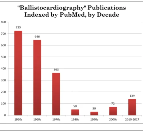
The use and study of ballistocardiography was booming after the TIME article was published but quickly faded away into obscurity as new contributions to cardiovascular medicine became more popular. The chart below demonstrates this decline in popular-ity. However, over the past couple of decades, ballistocardiography has been on the rise due to its non-invasive nature and potentially significant consequences as a result of new technologies. The time of Starr’s horizontal table may no longer be relevant, but with state-of-the-art weight measurement techniques, ballistocardiography can now possibly be used to determine vital information about a subject’s cardiovascular health [7].

(18)

FIGURE2.1: During the mid-20th century, ballistocardiography was in-tently studied which culminated in the publication of TIME magazine’s article. Soon after, it dropped off in popularity, only to reemerge in recent

years with the advent of newer technologies [7].

2.1.2 Mechanism

While it was known by the time Starr had published his article that the body recoiled due to the heart’s pumping, it was not known exactly why this was the case. Researchers had believed that the upward recoil was caused by the downward rush of blood through the aorta, but no other features of the ballistocardiograph (BCG) waveform could be ex-plained. With recent developments in technology, the BCG waveform and its multiple features can be obtained with greater detail. These features all have underlying mecha-nisms to explain their genesis [8].

Figure 2.2.1 below shows a typical waveform as measured by a BCG device over the course of a single cardiac cycle. The labelled peaks or valleys are each associated with some underlying physiological cause. Of all of the waves shown in the figure, the "I", "J", and "K" waves are the most notable. The "IJK" wave formed by these three peaks is what was detected by Gordon’s analog scale and Starr’s horizontal measurement table. The "I", "J", and "K" waves are typically seen as the most clinically significant aspects of the BCG waveform.

In their article about BCG, Kim et al. describe the mechanisms behind each feature within the BCG waveform [8]. By modeling the aortic arch as two separate components in series as shown in the figure below, an equation for the force detected by a BCG de-vice can be formed, shown in Equation 2.1. The two components in this model are the

(19)

2.1. Introduction 7

FIGURE2.2: The waveform shown here represents the total recoil experi-enced by the body during a single cardiac cycle. This BCG waveform is

composed of multiple peaks with varying underlying causes [8].

ascending and descending aortas which are depicted in series immediately following the left ventricle. In this equation, A is the average cross-sectional area of either the as-cending or desas-cending aorta, depending on the subscript. P describes the difference in blood pressure over time between different components of the aortic arch model. For example, δ P12refers to the difference in pressure between the ascending and descend-ing aortas, or P1- P2.

FBCG= ADδP12(t) −AAδP01(t) (2.1) The difference in blood pressure between these compartments is what drives the blood flow, and in turn, the features seen in the BCG waveform. The I wave is driven by a sudden increase in blood pressure at the onset of systole in P0while the ascending aorta is still in diastole. The peak of the I wave occurs when P01reaches its maximum value. While P1begins to increase and P2is still in diastole, the I wave begins its descent. The I-J upstroke occurs when P12 exceeds P01 and the J wave hits its maximum when P12 hits its peak. As P2 enters systole, the J wave transitions into the K wave. The K wave hits its peak once P12hits its minimum value. The L, M, and N waves are a result of similar interactions occurring due to effects of the dicrotic notch.

Since these waves are directly related to blood flow driven by pressure gradients, it is suspected that their amplitudes may be directly related to the stroke volume. It is not unreasonable to suggest that an increased stroke volume would be related to an increase in the amplitude of these waves. However, the exact nature of this relationship has remained elusive.

(20)

FIGURE2.3: The aortic arch can be modelled as the combination of the as-cending and desas-cending aortas connected to the left ventricle. The blood

pressures are labelled as Pxand the blood flow as Qx[8].

2.2 BCG Device

The device used to measure the BCG waveform is a modified weight scale combined with an electrocardiogram (ECG) handlebar as shown in Figure 2.4. The commercially available scale has been modified to turn on 45 seconds after non-negligible weight has been detected. The first 30 seconds is spent recording data and the final 15 seconds are used to write the data to an SD card. Once it is done with this process, the SD card can be removed from the device and read from using any SD card reader. The ECG handlebar is connected to the modified scale and the data is recorded simultaneously, resulting in synchronous measurements from the two devices. The BCG scale records at around 125 Hz, and the ECG scale samples at 1 kHz.

The ECG signal from the handlebar isn’t directly useful for its data, but is used to help synchronize the individual cardiac cycles in the BCG waveform. The reason this is done is that the BCG scale is extremely sensitive and often has significant beat-to-beat variation. However, typical BCG patterns begin to emerge when each of the BCG cardiac cycles are synchronized and ensemble averaged. The ECG signal is particu-larly useful in this step since the ECG handlebar detects electrical activity caused by the heart. When the heart’s ventricular muscles contract, the heart rapidly depolarizes. This depolarization can be seen as the "QRS Complex" on an ECG signal and is shown

(21)

2.2. BCG Device 9

FIGURE2.4: This device, obtained from Dr. Omer Inan at Georgia Tech, is a combination of a modified weight scale and ECG handlebar.

in Figure 2.5 below. The QRS Complex can be roughly seen as just prior to the onset of systole and can therefore be used to synchronize individual cardiac cycles by using the QRS Complex time stamp as the beginning of each cycle [9].

FIGURE2.5: The QRS Complex is the main feature of a typical ECG sig-nal and indicates the depolarization of the heart’s ventricles due to con-traction.

https://www.researchgate.net/figure/QRS-complex-of-ECG-signal_fig1_299405889.

When first obtained, the raw data from both the BCG and ECG are given in arbitrary units. The BCG waveform can be represented in Newtons using a known conversion. Since the ECG is only needed for its QRS Complex time stamps, it is instead simply nor-malized to the maximum R peak value. Once the raw data is converted, they are both filtered to remove any high frequency noise resulting from the circuitry or otherwise. The ECG signal is filtered through a band-pass filter that passes 10 to 25 Hz which is meant to emphasize the QRS Complex. The BCG waveform is filtered similarly with a band-pass that allows 0.8 to 15 Hz since the BCG waves are typically within this fre-quency band. After the filters are applied, a simple peak detection algorithm is run on

(22)

the ECG signal to find the R peaks and their time stamps recorded. After the peak de-tection, the time stamps are found in the BCG signal and the waveform for 0.6 seconds afterwards is recorded and saved as an individual cardiac cycle. When all of the indi-vidual cardiac cycles are recorded, they are ensemble averaged to produce a final BCG waveform for the subject.

2.3 Results and Discussion

All of the data shown in this section was obtained from a healthy male subject standing still on the scale with the handlebar held out with arms parallel to the ground. Once the data is recorded by the scale, the first step in obtaining the final BCG waveform is to acquire a clean signal from the ECG handlebar. This is shown in Figure 2.6 below, which displays the ECG waveform after applying the band-pass filter described in the previous section. The units on the y-axis are arbitrary units measured by the device and are normalized to the maximum R peak in the recording.

FIGURE2.6: The ECG waveform obtained from the handlebar is then sent through a band-pass filter that emphasizes the QRS Complex. It is clear to see the cyclic peaking in the ECG waveform caused by the QRS Complex.

Once the ECG signal is filtered and normalized, the peak detection algorithm will record at which times the R peaks occur. This algorithm will look for any peak ap-proaching the 1.00 value since all of the QRS Complexes in a given measurement should behave roughly the same. Occasionally, and depending on the subject’s grip on the han-dlebar, the QRS Complex will have a significantly reduced amplitude which will cause that cardiac cycle to be omitted from the final results. Once all of the time stamps for the R peaks are determined, then the individual cardiac cycles in the BCG waveform can be obtained using the methodology described earlier. Figure 2.7 shows all of the individ-ual BCG cycles as different colors with the thicker red line representing the ensemble average.

One noticeable aspect of the overlaid BCG cycles is that there is a significant amount of beat-to-beat variation due to the scale’s susceptibility to noise. This means that some cycles can have a very poor signal-to-noise ratio and are not ideal candidates for the ensemble averaging. To solve this problem, any BCG cycle that spends more than 10%

(23)

2.3. Results and Discussion 11

FIGURE2.7: The individual BCG cycles are shown as different colors with the thicker line representing the ensemble average. There is much

varia-tion between BCG cycles due to the scale’s vulnerability to noise.

of its time outside of one standard deviation from the average is removed. In the case of Figure 2.7, this simple algorithm would remove the black and blue cycles from the final ensemble average.

Once the final ensemble average is created as shown in Figure 2.8 below, certain fea-tures can then be extracted from the waveform. In this figure, the blue plot represents the ensemble averaged ECG waveform for all of the beats. Since the R peak in the QRS Complex represents the beginning of each cardiac cycle, this peak will represent t=0. The ensemble averaged BCG waveform more closely resembles the ideal BCG wave-form shown in Figure 2.2 compared to the individual BCG cycles. This is due to the fact that the ensemble averaging technique effectively reduces the effects of the noise and variability between cycles. Since we are looking for average stroke volume averaging out the variability is consistent with other averaging in the measurement and calcula-tion of the hemodynamic parameters.

There are multiple features associated with the BCG waveform that are thought to have some clinical significance: the IJ and JK amplitudes, IJ and JK intervals, the IJK width, and the RJ delay. The amplitudes are thought to give insight directly into the stroke volume since a larger volume of blood being pumped every cycle would produce a larger displacement of mass. The time intervals between features provide information regarding the contractile state of the heart, which has some relation to stroke volume. Measured values for these features are shown below in Table 2.1 and compared against those found in Inan’s work [10].

There is some debate as to whether the ensemble averaging technique is valid for clinical applications. Some cardiologists believe that using an averaged signal is not a viable representation of the subject’s cardiovascular health. Instead, it may be preferable to obtain the BCG parameters on a beat-to-beat basis and instead average those values. It is important to note that the BCG features of the ensemble averaged waveform are not necessarily equivalent to measuring those same features individually and averaging them. A visual demonstration of this concept is shown below in Figure 2.8. However, using the individual cycles may not be a good solution due to the effectively increased

(24)

FIGURE2.8: The final ensemble averaged BCG waveform is shown here. It resembles the ideal BCG waveform shown in Figure 2.2 and contains

all of the features therein.

BCG Feature Measured Values Literature Values IJ Amplitude [N] 3.62±0.84 4.06±1.53 JK Amplitude [N] 3.15±0.85 5.09±1.90 IJ Interval [ms] 81.0±10.9 94.7±21.2 JK Interval [ms] 92.0±18.4 98.4±1 4.5 RJ Delay [ms] 227.0±8.3 244.9±18.8

TABLE2.1: A comparison between values found using the device in this

work and those found by Dr. Omer Inan [10].

noise on the signal.

Another unfortunate factor caused by the sensitivity of the device is the effects of res-piration. During measurement, the subject’s breathing may cause non-negligible beat-to-beat variation on the BCG output. Since respiration occurs at a different frequency than the heart rate, its effects can be difficult to quantify. One solution is to have the sub-ject hold their breath during the BCG measurement. However, breath-holding exercises cause an initial increase followed by a more significant decrease in heart rate. Further-more, it causes vasoconstriction at the peripheries along with a decrease in blood flow [11]. For these reasons, breath-holding is not a viable solution and respiration cannot be decoupled from BCG measurements.

The next step in BCG research is to find out the relationship between the waveform and clinically significant parameters such as stroke volume. According to Dr. Inan, a multiple linear regression model can be created using IJ amplitude, IJK width, and the RJ delay along with the subject’s height and weight [10]. This analysis shows that these parameters have a correlation to stroke volume with an R2value of 0.60. This suggests that with enough tuning, BCG can be used to roughly estimate a patient’s stroke volume using entirely non-invasive methods. If this is true, then the device can be used to

(25)

2.3. Results and Discussion 13

FIGURE2.9: The colored shapes associated with BCG waveform features are shown either on the ensemble averaged waveform or floating around it. The ones that are floating represent the averaged values from the indi-vidual cycles as compared to those from the ensemble averaged cycle.

estimate the subject’s cardiac output since the heart rate is also known. Furthermore, developments in technology may allow measurements to be done with significantly reduced noise which would help with the fidelity of the BCG measurements.

(26)

(27)

15

Chapter 3

Ultrasound Background and Device

Historically, the use of medical ultrasound began shortly after World War II derived from underwater sonar research [12]. It was initially used to detect cerebral hematoma and brain tumors using simple one-dimensional technology. Today, medical ultrasound is used for three-dimensional imaging and a plethora of other applications. The remain-der of the this thesis will focus on ultrasound technology and how it can be applied non-invasively to determine clinically relevant parameters. This chapter will focus on some of the theory behind ultrasound and its application to the device that is used for the research.

3.1 Ultrasound Propagation and Scattering

Ultrasound is used to describe any sound wave with a frequency higher than the upper audible limit of human hearing. While the audible upper limit can vary from person to person, ultrasound is typically considered as anything above 20 kHz [13]. Ultrasound is used in medicine for imaging purposes but has multiple other industrial uses such as nondestructive testing and cleaning. For this study, ultrasound will be used for imaging along with a Doppler mode that will be described in a later section.

3.1.1 Acoustic Wave Propagation

Ultrasound, being a sound wave, requires a material medium in order to propagate. While propagating through gases or liquids, sound is transmitted through longitudinal waves. If it is transmitted through a solid, it can propagate as either a longitudinal or transverse wave. For human studies, the acoustic propagation material is often approx-imated as water since the water content in human tissue typically ranges from 50% to 80% [14]. This approximation is very useful since it is extremely difficult to characterize human tissue accurately and it simplifies the analysis to just the longitudinal wave.

An acoustic longitudinal wave propagates by creating zones of varying pressure within the medium. These are known as compression and rarefaction regions, which describe the areas of higher or lesser pressures compared to the equilibrium, respec-tively. The acoustic wave generates these pressure differences by displacing individual particles in the medium. When particles are displaced towards each other, the pres-sure is increased. The opposite is true when particles are displaced away from each other. The particle velocity can be found by analyzing the wave equation as shown be-low where u is the particle velocity and c is the propagation velocity, both in m/s. This

(28)

equation assumes a one-dimensional analysis of the acoustic wave. The wave equa-tion can be similarly solved in one-dimension for sound pressure by substituting u for pressure p [15]. The acoustic pressure has units of Pa.

∂2u ∂x2 − 1 c2 ∂2u ∂t2 =0 (3.1)

The wave equation requires the propagation velocity of the wave in order to solve. In keeping with the assumption that tissue is like water, the speed of sound can be found for liquids using the Equation 3.2 where K is the bulk modulus of the fluid and

ρis the density. The speed of sound in both water and body tissue is about 1540 m/s,

suggesting that the earlier approximation of tissue as water is valid [16]. c_liquid=

s K

ρ (3.2)

The acoustic wave has two more important parameters associated with it: acoustic impedance and intensity. The acoustic impedance is a representation of the opposition that a medium presents to the acoustic flow [13]. The impedance is calculated as the ratio between the acoustic pressure and particle velocity. Acoustic impedance has units of Pa·s/m.

Z= p

v (3.3)

Acoustic intensity I is defined as the power carried by the acoustic waves per unit area and as such will have units of W/m2[17]. Acoustic intensity is calculated by taking the product of the pressure and the particle velocity. Since it is calculated using the particle velocity, a vector, acoustic intensity is also a vector. It’s direction is typically given as normal to a specified unit area through which the sound energy flows. Acoustic intensity is an important parameter since it has no sound field dependence. Depending on the sound field, measuring simply the acoustic pressure to characterize an acoustic wave will result in failure. However, acoustic intensity has a direction associated with it and can be used regardless of the sound field through which is propagates [18].

~_I ₌ _p_~_v₌ p2 Z =

~v2

Z (3.4)

3.1.2 Ultrasound Interactions

As acoustic waves propagate through an inhomogeneous medium, they encounter two different phenomena: absorption and scattering [13]. The concept of scattering is ex-tremely important in medical ultrasound since the detection of a reflected acoustic wave is what drives ultrasound imaging. Acoustic absorption is the process by which the material medium transmitting the acoustic wave absorbs some acoustic energy. This energy is partially transformed into heat and the rest transmitted through the absorbing body. While absorption may be the main goal of soundproofing, it is not particularly ideal for medical ultrasound imaging where reflection is more desirable. Furthermore, the energy that is transformed into heat can present a medical hazard by possibly dam-aging tissue and must therefore be within regulatory limits. Since the acoustic wave

(29)

3.1. Ultrasound Propagation and Scattering 17 can only be absorbed or reflected, the absorption coefficient is calculated as shown be-low where IR is the reflected wave intensity and II is the incident wave intensity [13]. As absorption diminishes, reflected wave intensity approaches incident wave intensity . The strength of absorption depends on a multitude of factors such as the acoustic impedances of both media, the incident angle, and the frequency of the wave.

α=1− IR

II

(3.5) When an acoustic wave encounters a new medium, what is not absorbed is then scattered. The nature of the scattering is dependent on the characteristics of both the boundary and the incident acoustic wave. The three varieties encountered in ultrasound are specular scattering, diffuse scattering, and diffraction [19]. For medical ultrasound, specular scattering, also known as reflection, is typically the most desirable since simple reflection allows for imaging.

3.1.3 Specular Scattering

Reflection, or specular scattering, occurs when the roughness of the boundary is mul-tiple orders of magnitude geometrically greater than the wavelength of the incident wave, i.e. the wavelength is significantly smaller than the size of the rough features. For medical imaging, specular scattering occurs at the interface between tissue and bones, organs, or other large structures. Depending on the acoustic impedances of the two media at the boundary, some fraction of the incident wave will reflect and the rest will transmit. While the reflected wave will propagate at the same angle from the normal as the incident wave, the transmitted wave will propagate at a new angle based on Snell’s Law as shown in the figure below [20]. Snell’s Law states that this angle of transmission will be based on the incident angle and the velocity of propagation in each medium.

sin θ2 sin θ1

= c2 c1

(3.6) The reflection coefficient, or the ratio of the intensity of the reflected wave to the incident wave, is a measure of the difference between the two media at the boundary. While the reflection coefficient can be simply given as this ratio, it is more useful to de-scribe is using characteristics of the two media as well as the incident and transmission angles [21].

R= m cos θ1−n cos θ2

m cos θ1+n cos θ2, where m

= ρ2

ρ2, n

= c1

c2 (3.7)

ρ is the density and c is the speed of sound of the designated medium. The

trans-mission coefficient can then be described as 1 minus the reflection coefficient. After a reflection has occurred, the reflected wave will interfere with the incident wave. In this near field, the local pressure is not representative of either the incident or the reflected wave. However, at some distance away from the site of reflection in the far field, the effects of this interference are no longer significant.

(30)

FIGURE3.1: When an acoustic wave encounters a relatively featureless boundary, it will partially reflect and partially transmit. The angle of re-flection is equal in magnitude to the incident angle, but the transmitted

angle will be given by Snell’s Law [20].

3.1.4 Diffuse Scattering

Contrary to specular scattering, diffuse scattering requires that the new medium have a geometry on a scale below that of the acoustic wave’s wavelength. Specular scattering is useful in visualizing how the acoustic wave will interact when encountering a new tissue or other macroscopic object, but diffuse scattering is applicable when there are multiple microscopic scatterers within the medium through which the acoustic wave is propagating. Diffuse scattering results in a scattered waves propagating at multiple angles as shown in the figure below. Ideal diffuse scattering against a flat but rough surface causes equal luminescence at all angles in the half-space adjacent to the surface of reflection, also known as Lambertian reflection. This phenomenon is seen in medical ultrasound imaging when reflecting off of soft tissue where the adjoining cells create an uneven surface [19].

Most medical ultrasound devices range from 1 MHz to 10 MHz, so diffuse scatter-ing will happen against any surface smaller than 100 µm. Erythrocytes (i.e. red blood cells) have an approximate disc diameter of 8 µm and will create this type of scatter-ing behavior [13]. By approximating a red blood cell as a perfect sphere, it will exhibit Rayleigh Scattering which is often used to describe the reflection of light on particles much smaller than the wavelength of the light. The amount that is completely backscat-tered (i.e. at θ = π) is given by

Is Ii

= 25k

4_a6

36r2 (3.8)

where I is the intensity of either the scattered or incident wave, k is the wavenumber, a is the radius of the object, and r is the distance traveled by the reflected wave. Diffuse scattering is extremely important in this study for determining the blood flow velocity since the individual red blood cells will be reflecting the ultrasound waves with this kind of behavior. Red blood cells make up about 40% to 45% of the volume in blood and will contribute immensely to the total scattering seen by an incident ultrasound

(31)

3.1. Ultrasound Propagation and Scattering 19

FIGURE 3.2: When encountering an object smaller than the wavelength of the incident acoustic wave, the resulting re-flection will be spread out, known as diffuse scattering. https://upload.wikimedia.org/wikipedia/commons/b/bd/Lambert2.gif.

wave. However, erythrocytes are not the only source of diffuse scattering and the table below shows the attenuation coefficient of a 1 MHz ultrasound wave as it propagates through various media in the human body.

Body Tissue Attenuation Coefficient (db/cm at 1 MHz)

Water 0.002 Blood 0.18 Fat 0.63 Liver 0.5-0.94 Kidney 1.0 Muscle 1.3-3.3 Bone 5

TABLE 3.1: Various tissues and media throughout the human body are

riddled with microscopic scatterers that will cause an incident ultrasound wave to exhibit diffuse scattering. This type of scattering will attenuate

the propagating ultrasound wave [19].

3.1.5 Diffractive Scattering

Lastly, diffractive scattering occurs when the incident wave encounters an object or a slit with dimensions comparable to the wavelength. This kind of scattering is often associated with light experiments but also occurs with any type of longitudinal wave. If diffraction occurs, the scattered waves can be considered to originate at the scatterer surface which acts as a secondary source as shown in the figure below.

Towards the low end of ultrasound frequency (around 1 MHz), the wavelength is about 1 mm if propagating through human tissue or water. While this low-frequency ul-trasound wave is propagating through the inhomogeneous medium, it will experience

(32)

FIGURE3.3: When an incident acoustic wave comes across an object or slit with dimensions comparable to the wavelength, it will experience

diffraction [12].

diffraction when encountering any object or slit on the order of millimeters. The diffrac-tion pattern for acoustic waves only has dependence on the geometry of the scatterer and the wavelength, which is contrary to specular scattering which depends only on the mismatch of media at the boundary. For a spherical diffractive scatterer, the Born ap-proximation is often used to obtain the differential scattering cross-section [12]. Diffrac-tion is an important concept in ultrasound transducer design as well since a diffracDiffrac-tion pattern will result due to interactions with the ultrasound crystal within the transducer.

3.2 Ultrasonic Transducers

The systems that are used to generate ultrasound waves are known as ultrasonic trans-ducers. Transducers have specific geometry and electromechanical properties in order to create a specific ultrasound wave that is appropriate to the application and are, as such, important design considerations. Transducer geometry can be manipulated in modern systems to alter the diffraction pattern and allow for things such as beam fo-cusing and steering. In order to have these more advanced features, multiple transducer elements are utilized but a simple single element transducer will be discussed.

3.2.1 Ultrasonic Transducer Basics

The main goal of an ultrasound transducer is to take electrical energy and convert it into mechanical, or more specifically acoustic, energy and vice versa. In order to accomplish this, piezoelectric materials are used which can do exactly this type of energy transfor-mation [13]. One of the most commonly used piezoelectric materials used in the fabrica-tion of ultrasonic transducers is lead zirconate titanate (PZT), but is often times another crystal or ceramic [22]. Alternatively, capacitive micromachined ultrasonic transduc-ers, or CMUTs, have been gaining some traction in modern medical ultrasound but this study will focus on the use of piezoelectric elements only.

(33)

3.2. Ultrasonic Transducers 21 An ultrasound transducer consists of five main components as shown in the fig-ure below: the piezoelectric element, the electrodes, the damping or backing block, a matching layer, and the system housing [23]. The piezoelectric element is used to gen-erate an acoustic wave from an incoming voltage signal on its electrodes and vice versa. It must make use of the piezoelectric effect and the corresponding inverse effect in or-der to send and receive ultrasound waves. An alternating voltage signal excites the element, causing electric charges to accumulate at the electrodes which generates stress. This stress directly causes the vibration that forms the acoustic waves. Because of this, the frequency of the alternating voltage is equivalent to the frequency of the ultrasound waves. The geometry of the piezoelectric element is associated with the resonant fre-quency of the transducer. Since the thickness is significantly smaller than the other dimensions, it typically is the main contributor to the resonant frequency with a thicker element leading to a lower resonant frequency. A voltage signal driven at the resonant frequency of the transducer element is desirable to maximize the transmitted acoustic power.

FIGURE 3.4: A typical single element transducer will consist of five main components: the piezoelectric element, electrodes, damping block,

matching layer, and housing [23].

Since the piezoelectric element generates acoustic waves based on stress seen at its electrodes, it will actually propagate waves in both directions. For obvious reasons, a forward propagation from the ground electrode in the figure is desirable. However, a backwards propagating ultrasound wave will cause a backward transfer of energy and cause vibrations which may generate noise on the electrical signal output. The backing, or damping, block is meant to solve this problem by absorbing and attenuating the backward traveling acoustic waves. By reducing excessive vibrations, the element will be able to generate ultrasound waves with a shorter pulse length which improves

(34)

axial resolution (i.e. the image resolution along the direction of beam propagation). Unfortunately, this will reduce the overall efficiency of the transducer [12].

In medical ultrasound imaging, finer axial resolution is preferable as it will allow the device to differentiate between closely spaced scatterers. Axial resolution is directly correlated to an ultrasound transducer parameter known as the quality factor [12]. The quality factor is given as the ratio of resonant frequency to the half-power bandwidth,

δ f. δ f refers to the difference between the frequency above and below the resonant

frequency at which the intensity is reduced by a half. Q= f0

δ f, ARmin

≈ Qλ

4 (3.9)

As the quality factor increases, the efficiency of the ultrasound transducer also in-creases. However, it will also increase the axial resolution resulting in poorer image resolution. The backing material used to dampen the backward traveling acoustic wave will reduce the quality factor and efficiency. However, it will improve the image reso-lution so it is often desirable to have for medical imaging. On the other hand, Doppler ultrasound does not require fine axial resolution and will often prefer increased trans-ducer efficiency. The theoretical axial resolution given by the above equation will often lead to better predictions than in practice where second order effects will decrease effi-ciency.

Specular scattering occurs at the interface between two different media as described earlier. Since piezoelectric elements have a vastly different acoustic impedance com-pared to human skin, a massive reflection would occur at this boundary. To decrease the effects of reflection, a matching layer is placed against the piezoelectric element [23]. This matching layer is meant to act as an intermediate material between the element and the object, resulting in a reduction in reflection. This effect can be augmented through the use of ultrasound gel to ensure that a majority of the acoustic power is transmitted to the object of interest. Lastly, the housing provides electrical insulation and protects the piezoelectric element from external damage. The housing typically consists of a plastic case, a metal shield, and an acoustic insulator to reduce acoustic noise.

3.2.2 Ultrasound Beam Patterns

An ultrasound device can be operated in one of two modes: continuous wave (CW) or pulsed wave (PW). Medical imaging devices utilize PW due to the superior axial resolution. However, analysis of CW ultrasound is very useful in understanding the fundamentals of ultrasound. To generate CW ultrasound, a periodic waveform, typ-ically a sinusoidal or square wave, with an excitation frequency around the resonant frequency of the transducer is used. The beam pattern of CW ultrasound can be found by assuming the transducer surface consists of infinitesimal acoustic radiators all along the surface area of the transducer as seen in the figure below.

A beam pattern of this nature can be approximated using the Huygens-Fresnel prin-ciple which helps analyze both the near-field and far-field diffraction pattern [24]. Using this principle, each infinitesimal source is said to radiate equal spherical acoustic waves. The pressure contribution of each infinitesimal radiator is given by the equation below

dp= v0Z

λr0 cos

(2π f t−kr0+ π

(35)

3.2. Ultrasonic Transducers 23

FIGURE3.5: A cartesian representation of the transducer surface [24].

where v0is the amplitude of the surface vibration velocity, Z is the acoustic impedance, r0 is the distance from the infinitesimal radiator to the measured point, and k is the wavenumber [24]. Using the Huygens-Fresnel principle, the infinitesimal pressure can then be integrated along the surface of the transducer to obtain the pressure field.

p(~r, t) = Z Sdp = v0Z λ Z S cos(2π f t−kr0+ π 2) r0 dS (3.11)

This integral is known as the Rayleigh integral and is used to describe CW exci-tations [24]. The diffraction pattern caused by this pressure field can be separated into two regions: near-field, or Fresnel region, and far-field, or Fraunhofer region. Near-field refers to the region that immediately follows the transducer surface. In near-field, the in-finitesimal ultrasound elements cause constructive and destructive interference leading to a complicated and varying pressure field [13]. For these reasons, near-field is often times not the desired region of operation. However, there is a point where near-field transitions into far-field, known as the natural focus of the transducer.

z= a

2

4λ (3.12)

In this equation, a refers to the largest dimension of the transducer surface (diam-eter for a circular transducer). At this natural focus point, the acoustic waves are well behaved and are at maximum intensity. If the depth of the object of interest is known, placing it at the transition between near and far-field is often desirable if possible. How-ever, placing the object too deep in far-field can have consequences since the acoustic energy begins to diverge transversely and as such will have less acoustic power deliv-ered axially.

The simulated intensity fields for an ultrasound transducer with a circular aperture with a 5 mm at 2 MHz is shown in the figure above. This simulation does not take any attenuation into account. In the x-z plane, it is evident that the near-field has a much more complicated intensity field compared to far-field. Since the circular aperture has

(36)

FIGURE 3.6: A visualization of the beam diffraction pattern in near and far-field.

https://upload.wikimedia.org/wikipedia/commons/5/5d/FarNearFields-USP-4998112-1.svg.

only one dimension to it (the diameter), it has only one natural focal point. In a rectan-gular aperture, each dimension creates its own focal point which may be a consideration depending on the application.

While the continuous wave case is the classical treatment of ultrasound, it is often times not used in practice. In medical imaging, pulsed wave is commonly used due to the increased axial resolution it provides. The continuous wave analysis is useful to determine the beam’s diffraction pattern and effects of near and far-field, but gives no information regarding the time domain. This can be solved by using a generalized form of the Rayleigh integral, shown below [24]. In this equation, S denotes the transducer surface and v(~rs, t)is the time-dependent velocity normal to the transducer surface. This equation can be solved to formulate a time domain pressure waveform in space.

p(~r, t) = ρ 2π Z S ∂v ∂t(~rs, t− |~r0| c ) |~r0_| dS (3.13) 3.2.3 Doppler Ultrasound

An integral measurement for this research is to measure the blood flow velocity using ultrasound. This is accomplished using the Doppler effect. This phenomenon, first de-scribed in 1842, refers to a change in frequency of a wave created by a source that is moving relative to an observer [13]. This is most commonly observed with moving ve-hicles emitting sound waves that experience a Doppler shift when heard by a bystander. In the case of Doppler ultrasound, acoustic waves will be reflecting off of moving red blood cells and experiencing a Doppler shift which can be measured. Doppler ultra-sound can be employed using either continuous-wave or pulsed-wave. In both cases, the ultrasound beam must be insonated at an angle that has some component that is in

(37)

3.2. Ultrasonic Transducers 25

FIGURE3.7: The time-averaged intensity fields in the x-z at y = 0 mm (left) and x-y at z = 60 mm (right) planes are shown for a circular

trans-ducer with a 5 mm radius at 2 MHz [24].

the direction of the blood flow. Unlike imaging ultrasound, Doppler ultrasound can-not be used if the acoustic waves propagate perpendicularly to the blood flow. This is mathematically shown in the Doppler shift equation below

δ f = 2 f0v

c cosθ (3.14)

where δ f is the change in frequency in Hz, f0is the frequency of the insonated beam, v is the velocity of the object, c is the velocity of sound in the medium, and θ is the angle of insonation [12]. As the angle of insonation approaches 90 degrees, the Doppler shift approaches zero.

Continuous-wave Doppler ultrasound, as its name implies, continuously emits and receives ultrasound waves and is the simplest form of Doppler ultrasound. This is typ-ically done using two crystals, one for emitting and one for receiving. The ultrasound waves are emitted at a known frequency and then received at another frequency with the difference in frequency being measured. Using the above equation, the frequency shift can be related to blood flow velocity v. Unfortunately, the nature of this method impedes its ability to spatially separate incoming signals. Continuous-wave ultrasound observes all velocities within the sample volume that is pre-determined by the geometry of the system. Because of this, the scatterer location of an abnormal blood flow velocity measurement will be unknown [13]. However, this form of Doppler ultrasound has no restriction on scatterer velocities and is often used for high speed measurements at the aorta.

Pulsed-wave Doppler ultrasound uses short bursts to analyze the blood flow veloc-ity at specific depths from the transducer [25]. The transmitted and received acoustic waves are all handled by a single ultrasound transducer, an advantage over continuous-wave. Contrary to continuous-wave Doppler, pulsed-wave allows the sample volume to be restricted in the axial dimension because the round-trip time of the pulse contains information regarding the scatterer depth. Unfortunately, simple Doppler frequency shifts cannot be used in this method since the emitted signal is no longer a single fre-quency. Frequency dependent effects from the tissue can have a significant impact on

(38)

the received echo which makes it very difficult to determine the Doppler shift. How-ever, the round-trip time shift of the echo can be easily measured and also contains information regarding the scatterer velocity. This is due to the fact that the interaction of the wave with a moving object changes the round-trip time, which then changes the period, or equivalently, the frequency. Pulsed-wave Doppler ultrasound requires that a train of pulses be sent out at a frequency fPRF, or the pulse repetition frequency. In reconstructing the velocity waveform for the moving object of interest, the pulse repeti-tion frequency is the sampling rate. A common issue that arises with discrete sampling is aliasing, which is often mitigated by increasing the sampling rate. However, this is not entirely possible for PW Doppler ultrasound since the pulse repetition frequency must be slow enough such that a new pulse is not transmitted before the last one is re-ceived. Therefore, a maximum detectable velocity is enforced with PW Doppler and is expressed as:

Vmax=

c fPRF

4 f0cos(θ) (3.15)

More specific information regarding pulse-wave Doppler ultrasound can be found in Section 4.2.1 of the Seo Thesis [26].

(39)

27

Chapter 4

Hemodynamics

The end goal of this research is to obtain the hemodynamic parameters described ear-lier in the arterial system. The cardiovascular system is designed to provide organs and tissue with oxygen which is essential for function. More specifically, the arterial system delivers the oxygen and the venous system sends blood back to be oxygenated. The arterial blood flow is driven by the arterial blood pressure (ABP) created by the contrac-tion of the left ventricle. This pressure is propagated throughout the arterial system and eventually dissipated by the time it reaches the venous system. The exact dynamics be-tween arterial blood flow and pressure is very complicated and is often described using models. This chapter will lay down the foundation for the hemodynamics of the arterial system and provide motivation for the transmission line model discussed in Chapter 5.

4.1 Properties of Blood Flow

In dealing with flow in the cardiovascular system, it is common to only be concerned with physical laws governing the flow of liquids through solid tubes. Assuming for now that the tube is a rigid and uniform containing a non-turbulent, Newtonian liquid, the flow can be described using the Poiseuille equation:

P1−P2 =

Q∗µ∗L∗8

π∗ (R)4 (4.1)

where Q is the flow rate, µ is the viscosity, L is the length of the tube, and R is the radius [27]. This equation states that a pressure gradient along the tube is directly proportional to the flow assuming all other variables remain constant. However, the fluid velocity in the tube is not uniform due to the viscosity of the fluid. At the axis of the tube, the fluid will flow the fastest and the opposite is true at the walls. This is often illustrated using a series of laminae parallel to the walls of the tube and called laminar flow. While laminar flow adheres to the Poiseuille equation in most circumstances, it breaks down as the fluid velocity increases to a point where the resistance to flow begins to dominate. In this domain, the fluid is described as turbulent and the relationship between flow and pressure becomes unpredictable [27]. To describe any type of flow, it is imperative to know whether or not it is laminar or turbulent.

Several assumptions must be made to determine whether or not Poiseuille’s equa-tion applies. In the past, it has been debated extensively under which circumstances in the cardiovascular system this equation can be used. It has been concluded that as long as the blood sedimentation is negligible, it generally behaves under Poiseuille’s law [27]. However, in smaller capillaries, the viscosity of the blood depends on the radius

(40)

of the tube causing blood with a large number of erythrocytes to not obey Poiseuille’s equation. This equation can only be used to describe steady-state flow and is only truly valid in the terminal vessels of the arterial system such as capillaries. Even in arterioles, the flow is described as pulsatile and will exhibit different behaviors.

Early attempts at relating the blood flow to pressure in the arterial system were met with difficulties. Simple Windkessel models were used to describe the arterial system like a chamber in which the pressure rises as more blood is pumped into it [27]. This was useful for approximating the stroke volume but instantaneous flow rate could not be predicted. However, several studies have shown the viability of more advanced multi-element Windkessel models for estimating the relationship between pressure and flow [28]. For the most part, the observed blood flow and pressure waveforms are relatively synchronous as seen in Figure 4.1. It is important to note that the peaks are not in sync and that the flow waveform peaks slightly before the pressure waveform. This is due to the fact that pulsatile flow, like laminar flow, is driven by a pressure gradient and the flow peak occurs when the pressure gradient is at its maximum, which does not occur when the local pressure peaks.

Before the onset of systole in the arterial system, the blood can be thought of as at rest, something that is more true if the blood is proximal to the heart. When the pulse pressure is applied, the blood initially resists movement due to inertia but then begins to accelerate based on the pressure gradient. As the blood flow velocity increases, so does the viscous drag that resists the movement of blood. Due to the propagation of the pulse pressure, the gradient will eventually become negative and begin to decelerate the blood flow. In some arteries, the negative pressure gradient can result in a period of negative blood flow, which can be seen in the flow waveform in Figure 4.1. This phenomenon does not occur proximal to the heart due to the presence of valves that prevent negative flow.

In the case of pulsatile flow, Poiseuille’s equation cannot be used since it violates one of the requirements: steady rate of flow that is not subject to acceleration or deceleration. However, the pressure can still be related to the flow even in the case of pulsatile flow as seen below which was first tabulated by Womersley [29]. In his solution, which is detailed in his 1957 monograph, he first assumes that the pressure gradient only varies with time and can be written as Mcos(ωt−φ).

Q= πR 4_M µ M₁₀0 α2 sin(ωt−φ+e10α 2₌ R2ωρ µ [1−F10] =1− 2J1(αi3/2) αi3/2J0(αi3/2 (4.2)

In this pressure-flow relation, α is the Womersley number and M₁₀0 and e10 are the modulus and phase forms of the function [1−F10], respectively. In the equation for

[1−F10], J0 and J1 are the Bessel functions of order zero and one. When used in a situation where Poiseuille’s equation is applicable, M0₁₀/α2 goes to 1/8 and e10 equals 90◦ giving the relation seen earlier. Womersley’s solution is very useful in providing a pulsatile flow model that accounts for time-dependence. The Womersley number for an artery increases as its length scale increases, meaning that is is typically higher in arteries that are proximal to the heart [27].

(41)

4.2. Pulse Pressure Propagation 29

FIGURE 4.1: The pressure and flow waveforms are shown for a dog’s femoral artery. In the pressure waveforms, y represents the different

lam-inae [27].

4.2 Pulse Pressure Propagation

The above analysis of blood flow, both steady and pulsatile, describes a situation in which the fluid travels within a rigid tube. However, blood vessels are not rigid struc-tures and have viscoelastic properties that allow the diameter to vary with a pulsating pressure [27]. This allows for a finite propagation of pressure and flow through the ar-terial system when the left ventricle contracts since in a rigid system the pulse would travel infinitely fast. The speed at which the pressure and flow pulses propagate, known as the pulse wave velocity, is largely dependent on the elastic properties of the arterial wall and the fluid that flows within. This section will discuss the consequences of the viscoelastic properties of the arteries and of a traveling pulse pressure wave.

4.2.1 Arterial Wall Elasticity

No physical body can be described as perfectly rigid, or immune to deformations. The way a solid body reacts to an external force can allow it to be categorized as either elastic or plastic. If it is elastic, the body will return to its original form once the external force is removed. On the other hand, a plastic body will retain its deformation. Elastic theory often deals with how a body responds to such a force and how much it deforms. Stress is the force per unit area used to create a deformation and strain is the ratio of of the deformation to the original form of the body. A liquid under stress, such as blood

(42)

within an artery, will exhibit viscous flow. Any body that is described using elastic solid and viscous liquid properties is referred to as viscoelastic, and the arterial wall falls under this category.

An elastic material that experiences a tension (or force) applied to it will have a pro-portional change in length. For a cylindrical tube, the applied force is a circumferential tension in the wall created by a distending pressure P. In the case of an artery, this means that a pulse of pressure will cause the arterial wall to deform and expand. This expansion can be seen below,

dV dP =

2πR3

EhL−PR (4.3)

where R is the inside radius of the tube, E is Young’s Modulus, h is the wall thick-ness, and L is the length of the tube [27]. Assuming Young’s Modulus remains constant, the rate of increase of volume with pressure will increase until the pressure becomes EhL/R at which point the denominator goes to zero. When this occurs, the tube will burst or rupture. However, in the arterial wall, Young’s modulus increases as the cir-cumferential strain increases which allows arteries to stay intact even at high pressures. The above equation is not as simple as it seems since the thickness of the wall decreases as the artery expands and the length may not stay constant. A useful parameter in defining the viscoelastic properties of the arterial wall is its compliance. Compliance is defined as the change in volume for a given change in pressure, which is shown above in Equation 4.3. A similar parameter is the distensibility of an artery, which is defined as the compliance divided by the initial volume.

4.2.2 Wave Propagation

The elastic properties of the arterial wall are crucial for the propagation of the pulse pressure wave. The pulse wave velocity (PWV) can be found using an equation derived by Bramwell and Hill

PWV =

s VdP

ρdV (4.4)

where ρ is the density of blood and V is the arterial volume [26]. It is important to note that the PWV is not the same as the flow velocity of the fluid. This equation states that the PWV is related to the inverse square root of the compliance, or dV/dP. As the compliance approaches zero, the PWV becomes infinitely fast which is the rigid wall case. The Bramwell-Hill equation can be further simplified under the assumption that the tube has a thin wall (i.e. h/2R is small). This simplified form is known as the Moens-Korteweg equation [27].

PWV =

s Eh

2Rρ (4.5)

The Moens-Korteweg equation only works in situations where the tube has a thin wall and the fluid is incompressible and inviscid. However, in smaller arteries, the ef-fects of viscosity become more pronounced and will render this equation useless. More-over, if there is appreciable change in the wall thickness, the thin wall assumption is not

(43)

4.3. Vascular Resistance and Reflection 31 enough to use this equation. To solve this, corrections to this equation have been made that incorporate Poisson’s ratio to account for changes in wall thickness.

In the past, the PWV was measured to derive the compliance of a given subject’s artery. This was typically done by measuring the pressure waveform at two different points with a known distance apart and finding the propagation delay as shown in Figure 4.2. This can be done by analyzing either the flow or diameter waveforms, but it is generally easier to measure pressure. Older studies would use invasively mea-sured pressure waves to derive the PWV. However, more recent studies make use of non-invasive methods such as ultrasound or magnetic resonance imaging. Using these methods, a precise value for PWV can be found over short distances (< 10 cm). This can be attributed to energy loss mechanisms as well as shifting physiology that can accu-mulate over longer distances.

FIGURE 4.2: By measuring the pressure waveform at two points, the

PWV can be found by obtaining the propagation delay [27].

4.3 Vascular Resistance and Reflection

Similar to the impedance seen by traveling acoustic waves in ultrasound, blood flow likewise experiences resistance. The systemic vascular resistance mentioned in the in-troduction refers to the sum total resistance in the arterial network. Since it is not easy to model these resistances while remaining in the physiological domain, they are of-ten done using electrical analogies. These models can help in understanding various physiological phenomena such as reflection seen by the pulse wave.

4.3.1 Vascular Resistance

In the electrical analogy, pressure is like voltage, flow is like current, and vascular resis-tance is like electrical resisresis-tance. Historically, current was modelled using blood flow

Arterial blood pressure estimation using ultrasound technology and transmission line arterial model

Abstract

Acknowledgements

Contents

List of Figures

List of Tables

Chapter 1

Introduction

1.1

Motivation

1.2

Diagnostic Cardiology

1.3

Cardiovascular Parameters

Chapter 2

Ballistocardiography

2.1

Introduction

2.2

BCG Device

2.3

Results and Discussion

Chapter 3

Ultrasound Background and Device

3.1

Ultrasound Propagation and Scattering

3.2

Ultrasonic Transducers

Chapter 4

Hemodynamics

4.1

Properties of Blood Flow

4.2

Pulse Pressure Propagation

4.3

Vascular Resistance and Reflection