Terahertz radiations for breast tumour recognition

(1)

HAL Id: tel-03053722

https://tel.archives-ouvertes.fr/tel-03053722

Submitted on 11 Dec 2020

HAL is a multi-disciplinary open access archive for the deposit and dissemination of sci-entific research documents, whether they are pub-lished or not. The documents may come from teaching and research institutions in France or abroad, or from public or private research centers.

L’archive ouverte pluridisciplinaire HAL, est destinée au dépôt et à la diffusion de documents scientifiques de niveau recherche, publiés ou non, émanant des établissements d’enseignement et de recherche français ou étrangers, des laboratoires publics ou privés.

Quentin Cassar

To cite this version:

Quentin Cassar. Terahertz radiations for breast tumour recognition. Biotechnology. Université de Bordeaux, 2020. English. �NNT : 2020BORD0032�. �tel-03053722�

(2)

DOCTEUR DE L’UNIVERSITÉ DE BORDEAUX

DÉPARTEMENT DES SCIENCES PHYSIQUES ET DE L’INGÉNIEUR

SPÉCIALITÉ LASERS, MATIÈRE, NANOSCIENCES

présentée et soutenue publiquement par

Quentin C

ASSAR

le 25 Mars 2020

Terahertz Radiations for Breast Tumour Recognition

Directeur de thèse : Patrick MOUNAIX Encadrant : Jean-Paul GUILLET

Jury

M. Zimmer Thomas, Professeur des universités, IMS, Bordeaux Président

M. Gallot Guilhem, Directeur de recherche, LOB, Paris Rapporteur

M. Garet Frédéric, Professeur des universités, IMEP-LAHC, Chambéry Rapporteur

M. Peretti Romain, Chargé de recherches, IEMN, Villeneuve d’Ascq Examinateur

M. Pfeiffer Ullrich, Professeur des universités, IHCT, Wuppertal Invité

M. MacGrogan Gaëtan, Docteur en biopathologie, Institut Bergonié, Bordeaux Invité Mme. Tunon de Lara Christine, Docteur en chirurgie, Institut Bergonié, Bordeaux Invitée

(3)

(4)

The failure to accurately delineate breast tumor margins during breast conserving surgeries results in a 20% re-excision rate. Consequently, there is a clear need for an operating room device that can precisely define intraoperatively breast tumor margins in a simple, fast, and inexpensive manner. This manuscript reports investigations that were conducted towards the ability of terahertz radi-ations to recognize breast malignant lesions among freshly excised breast volumes. Preliminary works on terahertz far-field spectroscopy have highlighted the existence of a contrast between healthy fibrous tissues and breast tumors by about 8% in refractive index over a spectral window spanning from 300 GHz to 1 THz. The origin for contrast was explored. Results seem to indicate that the dynamics of quasi-free water molecules may be a key factor for demarcation. On these basis, different methods for tissue segmentation based on refractive index map were investigated. A cancer sensitivity of 80% was reported while preserving a specificity of 82%. Eventually, these pilot studies have guided the design of a BiCMOS-compatible near-field resonator-based imager operating at 560 GHz and sensitive to permittivity changes over breast tissue surface.

Keywords: Terahertz spectroscopy imaging; Biomedical engineering; Breast cancer; Data sci-ence; Inverse electromagnetic problem.

Résumé

(FR)-La faible précision avec laquelle sont délimitées les marges d’exérèse des adenocarcinomes mam-maires se traduit par un recours régulier à un second acte chirurgical. Afin d’en limiter la fréquence, la communauté scientifique tente de définir les grands axes de conception d’un système intraopératif permettant la reconnaissance des lésions mammaires malignes. Ce manuscrit de thèse rapporte les investigations menées sur la capacité des ondes térahertz à fournir un contraste entre tis-sus mammaires sains et malins. Les premiers travaux ont montré l’existence d’un contraste sur l’indice de réfraction entre 300 GHz et 1 THz, évalué en moyenne à 8%. Ce dît contraste semble prendre origine dans la dynamique des molecules d’eau intrinsèques aux cellules cancéreuses. Différentes techniques de segmentation d’image, basées sur l’indice de refraction des zones tissu-laires, ont permis de rapporter une sensibilité au cancer jusqu’à 80% tout en maintenant un taux de spécificité de l’ordre de 82%. L’ensemble de ces études a guidé la conception d’un imageur champ-proche opérant à 560 GHz, dont la réponse des différents senseurs est sensible à la per-mittivité en surface des tissus du sein.

Mots Clefs: Spectro-imagerie térahertz; Ingénierie biomédicale; Cancer du sein; Science des données; Problème électromagnetique inverse.

Université de Bordeaux

Laboratoire de l’Intégration du Matériau au Système (IMS) UMR CNRS 5218, F-33400 Talence, France

(5)

(6)

Resumes iii

Contents v

List of Figures vii

List of Tables xv Acknowledgments 1 Acronyms 3 Symbols 5 Medical Glossary 7 General Introduction 9

I Context and Key Concepts 13

I.1 Introduction . . . 14

I.2 Terahertz Radiations . . . 14

I.3 Terahertz Field and Biological Samples . . . 15

I.4 Breast Cancer . . . 39

I.5 Conclusion. . . 43

I.6 Bibliography . . . 44

II Terahertz Spectroscopy 53 II.1 Introduction . . . 54

II.2 Generation, Detection and Sensing . . . 54

II.3 Spectroscopy: Principles . . . 62

II.4 Water . . . 75

II.5 Phantoms . . . 80

II.6 Excised Breast Tissues . . . 89

II.7 Cancerous Cells . . . 99

II.8 Conclusion. . . 104

II.9 Bibliography . . . 105

III Terahertz Imaging: Far-field Survey 109 III.1 Introduction . . . 110

III.2 Far-field Imaging: Principles . . . 110

III.3 Self-Reference Image Inversion . . . 114

III.4 Image Registration . . . 121

III.5 Correlation. . . 124

III.6 Study Cases . . . 131

(7)

III.8 Conclusion. . . 160

III.9 Bibliography . . . 161

IV Breast Cancer Imaging: Near-field Survey 165 IV.1 Introduction . . . 166

IV.2 Beating the Diffraction Limit of Resolution . . . 166

IV.3 Towards a Silicon-Based Terahertz Near-field Imaging Matrix . . . 175

IV.4 Conclusion. . . 194

IV.5 Bibliography . . . 195

General Conclusion 199

Author Publication List 201

(8)

I.1 Location of the terahertz regime within the electromagnetic spectrum. . . 14

I.2 Refraction and reflection occurring at a dielectric interface between two media of propagation. . . 16

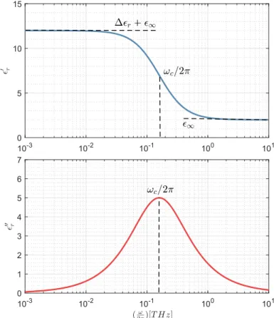
I.4 Example of a simple Debye treatment for∆²r−²∞= 12, ²∞= 2 and τD= 1ps. The in-flection point of²0r(ω) and the maximum of the dielectric loss factor ²00r(ω) are located atωC= 1.01 rad.ps−1.. . . 20

I.5 Illustration of the Cole-Cole treatment for the Debye parameters used in Figure I.4 (Top: blue; Bottom: red) and forα = 0.25,0.50,0.75 subsequently. . . 21

I.6 Illustration of the Cole-Davidson treatment for the Debye parameters used in Figure I.4 and forβ = 0.25,0.50,0.75 subsequently. . . 22

I.7 Illustration of the Havriliak-Negami formulation for the Debye parameters used in Figure I.4 and forα and β taking the successive values: 0.25, 0.50, 0.75. . . 23

I.8 Illustration of a Lorentz oscillator for²0= 75, A/(2π)2= 0.25 THz2,Γ/(2π) = 0.32 THz and a characteristic frequency atω0/(2π) = 500 GHz. . . 24

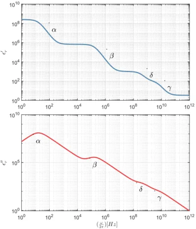
I.9 Schematic representation of the real and imaginary part of the relative permittivity, ²0 r and²00r as a function of the frequency and the location of the dispersive domains α, β, δ and γ. Where α denotes KHz relaxation of ions, β describes the MHz relax-ation of large biomolecules,δ depicts the hydration shell relaxation within protein surface - water complex andγ stands for bulk and free-water relaxations. Simulation performed by a tetra-Debye treatment (equation I.22 wherein N = 4) for²∞= 3.33, ∆²1 = 2.49 · 108, ∆²2 = 6.66 · 105, ∆²3 = 900, ∆²4 = 96.67, τ1 = 10−2s, τ2 = 10−6s, τ3= 5 · 10−10s,τ4= 5 · 10−11s. . . 25

I.10 Water molecules. Right: the bond network. Left: closer look on a hydrogen-bond and a covalent hydrogen-bond. . . 26

I.11 Structure of theα-form (left) and the β-form (right) of D-glucose. . . 28

I.12 Structure of the heparan sulfate polysaccharide subunit.. . . 28

I.13 Chemical structure of the fatty acid C16H32O2(palmitic acid).. . . 29

I.14 Schematic diagram of the DNA helix structure. . . 30

I.15 Protein synthesis in the ribosome complex. Proteins are assembled as stipulated by the encoded genetic information. The messenger-RNA (mRNA) serves as a template while the transfer-RNA (tRNA) acts as the physical link between the mRNA and the amino acid sequence of growing proteins. . . 31

I.16 Skin diagramm. . . 34

I.17 Eye anatomy.. . . 35

I.18 Tooth structure. . . 36

I.19 Breast anatomy. . . 40

(9)

I.21 Breast cancer surgery management: from initial partial mastectomy to second in-tervention, and histological examination in between. Step 1: abnormal tissue may extend beyond the visible fraction of the tumor. If not completely removed, the can-cer will recur. Step 2: The surgeon removes the visible portion of the tumor. Step 3: The excised tissue is formalin-fixed and paraffin-embedded. Then, the tissue is di-vided into thin section of around 5µm. Hematoxylin and eosin (H&E) stain is carried out to highlight cell cytoplasm and nuclei and the extracellular matrix. Hematoxylin stains cell nuclei blue, eosin staining pink the remainder of the section. Step 4: the pathologist microscopically examines the margins and the undersurface of each sec-tion. Step 5: if margins are defined as positive, the surgeon returns to the patient to remove the remaining abnormal cells.. . . 42

II.1 Illustrative example of pulsed terahertz generation by means of a photoconductive antenna. LCL: long carrier lifetime. SCL: short carrier lifetime. . . 55

II.2 Details of a free-space terahertz detection using aχ(2)susceptibility crystal. . . 57

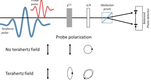
II.3 Reconstruction of a terahertz pulse by means of electro-optic sampling method. . . 58

II.4 Schematic details of a time-domain system for terahertz spectroscopy in transmis-sion configuration. BS stands for beam splitter, and M depicts mirrors. . . 59

II.5 Schematic details of a time-domain system for terahertz spectroscopy in reflection configuration. BS stands for beam splitter, and M depicts mirrors. . . 59

II.6 Illustrative terahertz time-domain waveform (blue) and spectrum (red) recorded through the use of a TDS setup. . . 60

II.7 Photograph of the TPS Spectra 3000 (left) and the Terapulse 4000 (right). . . 61

II.8 Scheme of the iterative determination of Ssam(ω). Each k-incrementation gives ac-cess to further possible events based on the previous ones at k − 1. Detected pulses have been marked with an eye in the node box. The incident angle was tilted for visual convenience. . . 63

II.9 Microscopic examination of the calibration sample. . . 64

II.10 Refractive index n( f ) and extinction coefficient k( f ) of each medium belonging to the calibration sample. . . 65

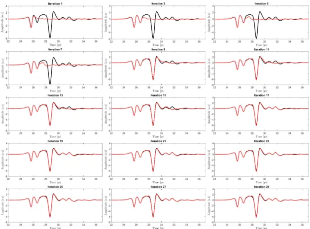
II.11 Progressive reconstruction of Sr(t ) (red) in comparison to the experimental signal (black) for the calibration sample made of four layers each of tens of microns. . . 66

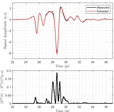
II.12 Top: experimental signal of the stratified structure in reflection geometry (black) and its reconstruction via the iterative tree algorithm (red). Bottom: deviations observed from the measured signal using theΛ(t) metric. . . . 67

II.13 Profile of the integrated comparison metric between 22 ps and 37 ps as a function of the number of iterations. The non-monotonous nature of the dependence reflects that time features are in majority due to the combination of several physical pro-cesses. Despite additional iterations, the error does not fall to zero. That is caused by unrecovered time features for the previously mentioned reasons and because time features corresponding to k → ∞ are basically out of the time window in which the comparison metric is defined. . . 67

II.14 Relative field at different frequencies as a function of the k−value and their respec-tive relarespec-tive noise level (dashed lines). The relarespec-tive noise level for each frequency is defined as the ratio of the noise level of the reference with respect to the reference field carried at these frequencies. The two dotted black lines represent the maximum and the minimum relative field value over the 0.2 - 2 THz spectral range observed at each k−value. Due to the dispersive behavior of coating layer, the difference be-tween the field carried at low frequencies and the field carried at high frequencies increases as k increases. . . . 68

(10)

II.15 Top: Reconstruction of the signal provided by the reduced iterative tree algorithm (black cross) with the 33 selected contributing paths (red). The correlation is almost perfect between the two signals over the entire time window. Bottom: Λ(t) metric. Differences are observed in regions where additional subdivided pulses have been

ommitted (e.g. k > 17). . . . 69

II.16 Representation of the main optical paths sorted by the iterative tree procedure for k-index ranging from 7 through 17. The optical paths at each k-values are sorted from left to right from the highest contribution to the signal to the lowest. Particular optical paths exhibit a symmetric one represented in dashed lines. These symmetric paths participate in an equivalent fashion to the signal. . . 70

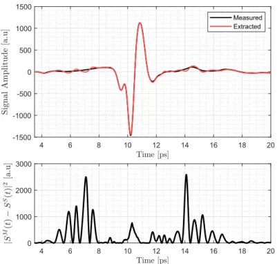
II.17Ptmax t =0 |SM(t )−SS(t )|2as a function of the tested thicknesses contained in the d vector. The global minimum was found to be 63.4µm. . . . 72

II.18 Time-domain error of the thickness global minimum using theΛ metric. . . 73

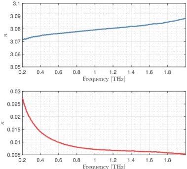
II.19 Optical properties n(ω) and κ(ω) for 63.4 µm. . . . 73

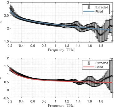
II.20 1st order Debye (i.e. n = 1 equation I.22.) fit of the IEP extracted properties. . . . 74

II.21 Reconstructed waveform after fitting the optical properties.. . . 75

II.22 Refractive index and extinction coefficient of the sapphire substrate. . . 76

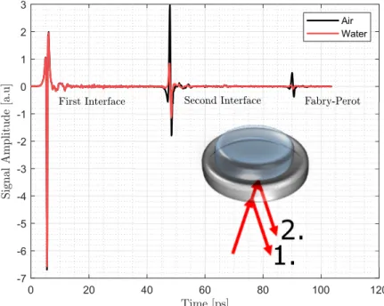
II.23 Typical time-domain waveform recorded without (black) and with (red) water film on the top side on the sapphire substrate.. . . 77

II.24 Water optical properties extracted in reflection geometry, averaged over ten inde-pendent measurements. . . 77

II.25 Cole-Cole plot of water and approximated representation of characteristic relaxations domains. In black dashed lines are schematically represented the portion of the semi-circle that describes the double-Debye relaxation nature. Frequency axis de-creases from 200 GHz to 1 THz from right to left. . . 78

II.26 Residuals at eachω with respect to both the real and complex plane for 2-Debye terms and 3-Debye terms. . . 79

II.27 Fit to 2-Debye terms model and the experimental n(ω) and κ(ω). . . 80

II.28 Frequency dependence of the refractive index and the extinction coefficient of each samples. . . 82

II.29 Fitting of the dispersion profiles of each phantoms with respect to II.33. Blue: #1 phantom; Green: #3 phantom; Yellow: #4 phantom; Purple: #5 phantom. Black dashed line represents theΛ metric. . . 85

II.30 Fitting of the real part of the dispersion profiles of each phantoms. Blue: #1 phan-tom; Green: #3 phanphan-tom; Yellow: #4 phanphan-tom; Purple: #5 phantom. Black dashed line represents theΛ metric. . . 87

II.31Λ metric on the comparison between Truong et al model and the modified-Lorentz one for phantoms. Blue: #1 phantom; Green: #3 phantom; Yellow: #4 phantom; Purple: #5 phantom. Black dashed line represents theΛ metric. . . 89

II.32 I.I and K.I samples sandwiched between two sapphire substrates to prepare the tis-sue measurement. . . 91

II.33 Refractive index and extinction coefficient for malignant lesions, healthy fibrous and adipose tissues. . . 91

II.34 Refractive index and extinction coefficient difference between adipose and healthy fibrous as a percentage of healthy fibrous characteristics. . . 93

II.35 Refractive index and extinction coefficient difference between healthy fibrous and cancer as a percentage of cancer characteristics.. . . 94

II.36 Fitting of the dispersion profiles of the mean response of cancer (solid red), fibrous (solid blue) and adipose tissue (solid green). Dashed black line represents theΛ met-ric between measurement and fitting. . . 96

II.37 Averaged distribution of model parameters of each poles for tissue types.. . . 98

(11)

II.39 Dispersion profiles of the real and imaginary part of the dielectric constant for each cell concentration. . . 101

II.40 Variations in²_∞,∆²1and∆²2as a function of MCF7 cell concentration. . . 103

II.41 Contribution of²∞, ²1and²2to the dielectric constant dispersion profiles. . . 104

III.1 Schematic representation of the information volume acquired during 2D material imaging. The third axis, t represents the time. . . . 111

III.2 Abbe’s limit between 200 GHz and 1 THz in free space forθ0=π₆. . . 112

III.3 Resolution test-target. . . 112

III.4 Minimum resolved spatial frequency corresponding to at least a contrast of 30% as a function of the sensing terahertz frequency. . . 113

III.5 Smallest resolved line pairs (dashed red square) for 200, 400, 600, 800 and 1000 GHz. The smallest resolved spatial frequency at 200 GHz was assumed to be half the spatial frequency of group -2, element 1.. . . 114

III.6 Flow chart to illustrate the procedure to improve sample characterization. R1and R2

depicts the lower and upper reflected pulses at dielectric interfaces. . . 115

III.7 Schematic illustration of the plane of interest that contains the information about the tissue sample. . . 116

III.8 Example of a typical pixel that allows the reference retrieval. . . 116

III.9 Scaling function and shape of the db6 wavelet. . . 118

III.10Block diagram of the self-reference method. (i). A retrieval pixel is selected; (ii). Sig-nal inversion is performed to calculate the reference sigSig-nal; (iii). The reference sigSig-nal is denoised by means of db6 wavelet. Eventually, the complete signal of the retrieval pixel arising from the interaction of the calculated reference with the two dielectric interfaces is retrieved. Note that the time-scale is relative rather than absolute. . . . 119

III.11Representation of a pixel with the four associated pointel (0;0), (0;1), (1;1), (1;0) and the four linels joining them. . . 120

III.12Illustration of the contouring procedure to reduce the number of pixels treated by the inverse electromagnetic problem. (i). Raw terahertz image of a sample; (ii). Contour levels extraction; (iii). Enclosed surface associated to a selected contour level; (iv). Delineation of the region to be treated by inverse electromagnetic problem. In the example, the number of pixel to be considered was reduced from 101,440 pixels to 56,296 pixels.. . . 121

III.13Problems associated with 2D histological images. (a) Presence of tears and holes. (b) Global shape deformation and missing information. (c) Artefacts in and around. (d) Glue deposited on sample slide. (e) Local misalignment of tissue substructures. (f ) Vignette arising from difference of thickness around tissue edges. Reproduced with the courtesy of Abiodun Ogunleke [20]. . . . 122

III.14Representation of the registration process. The terahertz and pathology original im-ages are treated by a contouring algorithm to extract the edges of each image. The pathology image resolution is reduced to match the lower resolution of the terahertz image. Then, the terahertz image is reoriented with respect to the pathology image until the best correlation is achieved. These modifications are therefore applied to the refractive index map and the pathology mask. . . 124

III.15Representation of the refractive index thresholding. a. Schematic refractive index map. b. Refractive index thresholding for t = 2.4. c. Refractive index thresholding for t = 2.1. d. Refractive index thresholding for t = 1.8. . . . 125

III.16Spreading of an object due to PSF. From left to right: punctual object, PSF and spread object image. . . 126

III.17Representation of the class overlapping for the modulus amplitude distribution C1

(blue) and C2(orange). Green fills the overlapping region where it is not possible to

clearly define pixel’s belonging. Black curve represents the sum of the two distribu-tions and therefore the observed global behavior. . . 126

(12)

III.18Schematic representation ofΣ1 andΣ2structuring elements. Left: Σ1 structuring element that may also be named local connectivity with four connectivity. Right:Σ2 structuring element that is not solely local as it consists of twelve connectivity pixels. 128

III.19Diagram of the classification process from the refractive index map to both the hard and connected thresholding diagnosis. The black dashed arrow on the top of the di-agram refers to the inverse electromagnetic problem (IEP) and upstream data treat-ment performed to derive the refractive index map. Note that it is possible to think about connected thresholding as an expansion of the hard thresholding rather than an independent process. For clarity purposes, the two strategies have been organ-ised in two distinct arms. Black dashed circles highlights . . . 129

III.20Flow chart of the method followed to classify tissue section terahertz pixels.1: Note that the histology treatment is performed after the terahertz imaging. . . 131 132figure.caption.148

III.22Receiver operating characteristic for the different classification methods, at 560 GHz. The black line represents TPR = FPR. . . 133

III.23TPR − FPR as a function of the refractive index threshold for HT, CT1, CT2 and CT3, at 560 GHz.. . . 134

III.24NS1 tissue sample classification map at 560 GHz for HT, CT1, CT2 and CT3 and their respective first two best thresholds, at 560 GHz. . . 136

III.25Overview of the results obtained via the procedure for the NS2 sample: i. photo-graph; ii. pathology image with four enlightened regions. A gap is shown in the middle of the section that is due to the histology chain; iii. Pathology mask derived from the pathologist diagnosis. iv. Terahertz image of the tissue sample at 560 GHz; v. Terahertz mask derived from the 560 GHz raw image; vi. Refractive index map cal-culated from the self-reference procedure and the inverse electromagnetic problem; vii. Raw and denoised retrieval pixel signals used to retrieve the reference signal -relative time-scale; viii. Reconstructed signal from the retrieval denoised pixel signal - relative time-scale. a, b, c and d are pathological view of the regions related in the pathology image (ii) and the raw terahertz image (iv). . . 137

III.26Receiver operating characteristic for the different classification methods, at 560 GHz. The black line represents TPR = FPR. . . 138

III.29Overview of the results obtained via the procedure for the NS3 sample: i. photo-graph; ii. pathology image with four enlightened regions. A gap is shown in the middle of the section that is due to the histology chain; iii. Pathology mask derived from the pathologist diagnosis. iv. Terahertz image of the tissue sample at 560 GHz; v. Terahertz mask derived from the 560 GHz raw image; vi. Refractive index map cal-culated from the self-reference procedure and the inverse electromagnetic problem; vii. Raw and denoised retrieval pixel signals used to retrieve the reference signal -relative time-scale; viii. Reconstructed signal from the retrieval denoised pixel signal - relative time-scale. a, b, c and d are pathological view of the regions related in the pathology image (ii) and the raw terahertz image (iv). . . 142

III.30Receiver operating characteristic for the different classification methods. The black line represents TPR = FPR, at 560 GHz. . . 143

(13)

III.34Schematic representation of a data matrix to be inserted into the PCA routine.. . . . 149

III.35Integrated loading weighted frequencies for modulus and phase data set for the first three principal components. The reader is referred to Figure III.21 for eyeball com-parison.. . . 151

III.36Modulus data set projection on the PC1-PC2-PC3 space. a) 3D projection on PC-PC2-PC3 space. b) PC2(PC1) projection. c) PC3(PC1) projection. d) PC3(PC2) pro-jection. . . 152

III.37Phase data set projection on the PC1-PC2-PC3 space. a) 3D projection on PC-PC2-PC3 space. b) PC2(PC1) projection. c) PC-PC2-PC3(PC1) projection. d) PC-PC2-PC3(PC2) projection. 153

IV.1 Delineation between the near-field domain and the far-field regime. The near-field regime is defined as the sphere of radiusλ/2π whose center is the punctual electro-magnetic source. Beyond the near-field sphere, interactions with matter should be regarded as far-field effects. . . 167

IV.2 Near-field sensing with terahertz source near the sample to be inspected. a: ap-proach developed by Lecaque et al in [5;6]. The sample is placed on the emitter. b: coupling between an optical fiber and aχ(2)crystal as reported by [7] . . . 168

IV.3 Near-field sensing with terahertz detector near the sample to be inspected. a: ap-proach developed by [9]. The terahertz field induces a refractive index change in the electro-optic crystal onto which is mounted the sample. Polarization ellipticity changes in the counter-propagating probe fs-laser beam are recorded. b: alterna-tive idea suggested by [11] where the electro-optic crystal is replaced by H-shaped electrodes patterned on a silicon layer. . . 170

IV.4 Near-field sensing with both terahertz electro-optic source and detector close to the sample to be inspected [12].. . . 170

IV.5 Near-field sensing with illuminated sub-wavelength aperture. Note that the sample may either be upstream or downstream the sub-wavelength aperture. a: the tera-hertz beam passes through the sample and subsequently through a sub-wavelength gold aperture. The electric component of the transmitted field is detected by a low temperature grown GaAs photoconducting antenna [15]. b: the incident terahertz beam is sent onto a bull’s eye structure that activates surface waves. The resonant excitation of those waves allow to increase the amplitude of the electric field that is detected. Terahertz passes through a bow-tie aperture and interacts with the inves-tigated sample [17]. . . . 171

(14)

IV.6 Scheme of a S-NSOM setup. A terahertz beam is focused onto the sample surface by means of lenses. The evanescent field is probed with an oscillating scatterer that vibrates at the frequency of the field to be recorded. The measurement of the near-field suffers from the inavoidable presence of a strong far-near-field background. . . 173

IV.7 Conceptual design of a near-field device that senses the evanescent field arising from the interaction of terahertz radiations with a sample (right). The device is aimed to consist of an illumination source, a near-field surface sensor and a high-responsivity terahertz power detector, with all mounted on an unique chip. Thanks to subwave-length resolution, features whose size is smaller than the probing wavesubwave-length can be resolved. a: the smallest size of features than can be resolved depends on the near-field device performances. In comparison, far-near-field probing (left) does not allow to resolve sample features smaller thanλ/2. . . 175

IV.8 Representation of different split-ring resonator geometries. a: circular SRR; b: dou-ble circle SRR; c: complementary spiral SRR; d: square SRR; e: U-shaped SRR; f: dual-square SRR. . . 176

IV.9 Schematic representation of a split-ring resonator probe. The resonator behaves like a LC-component whose characteristic frequency is about to be shifted in the pres-ence of a sample, at the neighborhood of the resonator gap. . . 176

IV.10Block-diagram of the measurement operation. The resonance shift is interpreted as amplitude transmission changes from opaque to lucent at the terahertz power detector output. . . 177

IV.11Sensor scheme. a: 3/4 view of the complete sensor made of a transmission line, and cross-bridged dual-square SRR; b: top view of the resonator with L = 19µm, W = 4.5 µm, and S = 3 µm.. . . 178

IV.12S21 parameter profile between 400 GHz and 600 GHz highlighting the presence of

a nominal resonance frequency (ω0

2π) at 540 GHz. The sensor illumination (ω2πosc) is

proceeded at 560 GHz. . . 179

IV.13Profile of S21as a function of the PEC distance from the surface. Left: Highlight of

the induced frequency shift due to the PEC relative altitude. Right: Bi-exponential behavior of S21as a function of the PEC relative distance at 560 GHz, withα1= -6.273,

α2= 0.099,β1= 4.082 andβ2= -1.189. . . 180

IV.14Profile of S21as a function of different²0. Left: Highlight of the induced frequency

shift due to the progressive increase of²0. Right: Bi-exponential behavior of S21as a

function of the²0relative permittivity at 560 GHz, withα1= -6.675,α2= -0.488,β1=

-5.755 andβ2= -0.038. . . 181

IV.15Profile of S21as a function of different²00. Left: Highlight of LC-circuit response due

to the progressive increase of²00. Right: Bi-exponential behavior of S21as a function

of the tanδ relative loss angle at 560 GHz, with α1= -9.677,α2= -0.029,β1= 0.041 and

β2= -10.55. . . 181

IV.16Slope as defined in equation IV.7 as a function of t anδ with α1= 0.106,α2= -1.761,

β1= 0.255 andβ2= -0.371. . . 182

IV.17Profile of S21as a function of²0and²00. Left: Highlight of LC-circuit response due

to changes in²0 and²00 . Right: Map of the S21value at 560 GHz for²0∈ [1; 6] and

tanδ ∈ [0;0.5]. . . 182

IV.18Profile of S21for water methanol, ethanol and propanol. Left: Highlights of the

LC-circuit response to polar liquids. The inset depicts the values of²0 and²00for each sample at 560 GHz as derived from the parameters in Table IV.1. Right: Behavior of S21at 560 GHz as a function of the considered liquids. Simulated differences in S21

(15)

IV.19Profile of S21for water, BCC, normal and adipose tissue. Left: Highlights of the

LC-circuit response to biological tissues. The inset depicts the values of²0 and²00for each tissue types and water at 560 GHz as derived from the parameters in Table IV.3. Right: Behavior of S21at 560 GHz as a function of the considered tissues. Simulated

differences in S21between the different samples are highlighted.. . . 185

IV.20Micrograph of the near-field sensing array. The sensing strip length is 3.2 mm long. The black region contains additional circuits that are not associated to the near-field sensing. ASIC: application-specified integrated circuits. ADC: analog-to-digital con-verted. Refgen: reference generator. BP: bandpass. . . 186

IV.21Block diagram of the system on a chip with the required external components. The chip contains 2 rows of 64 pixels, each divided into 16 subarrays of 4 entities illu-minated by a common oscillator and an on-chip lock-in amplifier read-out. Pixel selection (row,col)) is achieved via an application-specific integrated circuit (ASIC). adlccl k: analog-to-digital converter clock. FADC: flash analog-to-digital converter. GND: ground. LIref: lock-in reference. OSC: oscillator. TP: test point. UART: uni-versal asynchronous receiver/transmitter. VDD: digital supply voltage. VCC: analog supply voltage.. . . 187

IV.22Photograph of the packaged imaging module. a: 3/4 view of the module with 1-euro coin for scale. b: top view of the module, highlighting the sensing line, the spacer and the wire bonds encapsulated in epoxy resin. c: zoom on the system on-chip (x20).188

IV.23Surface profile analysis of a small fraction of the sensing strip. Strip lines are elevated by about 12µm. Such a topology makes it difficult to accurately sense stiff material as a perfect control of the altitude and the flatness with respect to the sensing line are required. . . 190

IV.24Droplet deposited onto the top of the sensing line. . . 190

IV.25Response of the near-field array pixels as a function of the deposited liquids to that of free space. a: global matrix response to water. b: global matrix response to methanol. c: global matrix response to ethanol. d: global matrix response to propanol. Loga-rithmic scale in arbitrary units. The reader is invited to note that the scale is loga-rithmic rather than linear to highlight matrix response difference between liquids.

. . . 191

IV.26Pixel response to water (blue), methanol (red), ethanol (green) and propanol (yel-low). The mean level of propanol is slightly lower than that of ethanol. The mean level of the matrix response to methanol is higher than for other liquids. Water stands in the middle as a result of the impact of its lossy part of permittivity. . . 192

IV.27Biometric fingerprint data comparison [35]. a: ink-and-paper fingerprint. b: 560 GHz near-field image of the equivalent finger region. Points 1, 2 and 3 depict the presence of ridge splitting that are well retrieved from ink-and-paper fingerprint to terahertz image. . . 193

IV.28Terahertz near-field imaging of a deparaffinized breast section [35]. a: micrograph of the deparaffinized imaged breast section; b: height profile of the sample; c: terahertz near-field image at 560 GHz with the section in contact with the array. . . 194

(16)

I.1 Dielectric properties of some alcohols and water at 70 GHz. [28] . . . 19

I.2 Comparison of the dielectric Debye parameter for water molecules found in the lit-erature. a_{Parameter fixed during the Levenberg–Marquardt fitting procedure [}₄₁_;₄₇_]. b In-cludes intermolecular libration amplitude. . . 27

I.3 Relative mass (%) of water, lipid, protein, carbohydrate for various body tissues [66]. a_{: Approximations are particularly schematic for breast composition since} compo-nent content varies among individuals and tissue excision location [67]. In addi-tion, significant variations in composition have been observed for adipose tissue and mammary glands as reported by [66]. . . . 33

I.4 Cancer classification system. Cancers are sorted by histological appearance. De-pending on the histological type, they are classified as ductal or lobular carcinoma. Carcinoma in situ denotes cancers which have not spread out the initial tissue com-partment, while invasive carcinoma have spread in surrounding tissues. The grade states for the differentiation level of cells. Tissues exhibiting cells least like normal ones are by and large high grade carcinomas. . . 41

II.1 Properties of some ultrafast photoconductive substrates for pulsed terahertz emission. 56 II.2 Characteristics of the TPS Spectra 3000 and the Terapulse 4000. . . 61

II.3 Fitting Debye parameters for the four coatings of the calibration sample.²_∞stands for the dielectric constant at high frequencies,∆² is the permittivity difference be-tween the static dielectric constant and the relaxation process permittivity, occurring over the timeτ. d stands for the thicknesses extracted from optical measurement. . 65

II.4 Number of computed paths for each k-incrementation and the number among them outgoing the structure being thus detected. . . 68

II.5 Fitting Debye parameters for the unknown sample. . . 74

II.6 Fitting parameters for 2-Debye terms and 3-Debye terms. . . 79

II.7 Fraction of protein, oil and water in each phantom in percent-by-weight.. . . 81

II.8 Fitting parameters of each phantom with respect to equation II.33. . . 84

II.9 Fitting parameters of each phantom for (II.36a). . . 87

II.10 Parameters of the model proposed by Truong et al. aR2 is the adjusted R-square value denoting the square of the correlation between the response values and the simulated ones. When equal to unity, the adjusted R-square value denotes a per-fect correlation while being equal to 0 it denotes a null correlation. BCC: basal cell carcinoma. . . 88

II.11 List of the fifteen freshly excised tissues analyzed in reflection spectroscopy. Samples having the same letter reference code belong to the same patient and have been ex-cised during the same procedure. The diagnosis column refers to the pathology from which is suffering the patient. ILC: invasive lobular carcinoma; IDC: invasive ductal carcinoma; MBC: metaplastic breast cancer; BPT: breast phyllodes tumor; BR: breast reduction. . . 90

(17)

II.12 Fitting parameters for the mean complex dielectric function of each tissue types for

(II.33).. . . 95

II.13 Comparison of²_∞. . . 97

II.14 MCF7 cell concentrations. . . 100

II.15 Debye parameter for the best fitted relaxation strengths. . . 102

III.1 Thickness and spatial frequency of each element of the USAF-1951 test-chart. . . 113

III.2 Compliance decision rule between the terahertz image and the pathology one. . . . 130

III.3 Area under the curve for each classification method. . . 133

III.4 First two best refractive index threshold characteristics considering the trade-off be-tween TPR and FPR. . . 134

III.5 Area under the curve for each classification. . . 138

III.7 Area under the curve for each classification. . . 143

III.9 Contribution to variance (%) for the first six principal components based on the modulus and the phase of each pixel between 200 GHz and 1 THz.. . . 150

III.10Contribution to variance (%) for the first six principal components based on the modulus and the phase of each pixel between 200 GHz and 1 THz.. . . 154

III.11Contribution to variance (%) for the first six principal components based on the modulus and the phase of each pixel between 200 GHz and 1 THz.. . . 157

IV.1 Debye parameter of water, methanol, ethanol and propanol as used to simulate their respective dispersion profiles.. . . 183

IV.2 Simulated sensor response to water, methanol, ethanol and propanol. Values are given with respect to that of free space. P00/P₀denotes the gain in transmitted power for a particular sample with respect to that of free space.. . . 184

IV.3 Parameters of the model proposed by Truong et al. aR2 is the adjusted R-square value denoting the square of the correlation between the response values and the simulated ones. When equal to unity, the adjusted R-square value denotes a perfect correlation while being equal to 0 it denotes a null correlation. . . 185

IV.4 Simulated sensor response to basal cell carcinoma (BCC), normal fibrous and healthy adipose. Values are given with respect to those of free space. P00/P₀denotes the gain in transmitted power for a particular sample with respect to that of free space.. . . . 185

IV.5 Simulated sensor response to water, normal fibrous and healthy adipose. Values are given with respect to those of basal cell carcinoma (BCC). P00/P_BCCdenotes the change in transmitted power for a particular sample with respect to that of BCC. . . 186

IV.6 Permittivity lossless and lossy part for water, methanol, ethanol and propanol at 560 GHz from [36] and this work. . . . 190

(18)

Je souhaiterais avant tout remercier Dr. Patrick Mounaix, mon directeur de thèse, pour m’avoir laissé me tromper. C’est ainsi -je crois- que j’ai pu tant apprendre et ne jamais cesser de question-ner.

Mes sincères remerciements aux Dr. Jean-Paul Guillet, Dr. Thomas Zimmer et Dr. Gaëtan MacGrogan, qui m’ont tous trois permis de progresser dans chacun de leur domaine d’expertise respectif. Au même titre, j’aimerais remercier M. Frédéric Fauquet, pour sa gentillesse et son ent-housiasme permanent à l’égard de mon travail.

Mes pensées vont également au Dr. Christine Tunon de Lara, engagée au sein de ce projet en tant qu’experte en chirurgie du sein.

Mein Dank gilt auch dem gesamten Forschungsteam in Wuppertal, unseren Partnern in diesem Projekt und insbesondere Prof. Ullrich Pfeiffer und Philipp Hillger für ihre Erläuterungen und Hilfe bei der Nutzung der Nahfeldmatrix.

Je souhaiterais également remercier le Dr. Guilhem Gallot et le Dr. Frédéric Garet pour avoir acceptés de participer au processus d’évaluation de mon mémoire de thèse en tant que rappor-teurs, ainsi que le Dr. Romain Peretti pour le temps accordé à mon travail en tant qu’examinateur de ces travaux.

Je souhaite également remercier M. Samuel Caravera, technicien supérieur à l’institut Bergonié, centre régional de lutte contre le cancer, pour son enthousiasme et sa patience à l’égard de mes de-mandes concernant les échantillons excisés, même les plus farfelues. C’est également l’ensemble des équipes à Bergonié qu’il me faut remercier, je pense à Marie-Claude, Reynlad, Fabien, Valérie et Stéphane.

Il me faut adresser mes sincères remerciements à Mme. Florence Poulletier de Gannes, pour sa patience et son aide concernant la culture des cellules MCF7.

Mes pensées vont à Amel Al-Ibadi, Joyce Bou-Sleiman et Corinna Koch-Dandolo, avec qui j’ai pu, de près ou de loin travailler sur diverses thématiques.

Хочу выразить искреннюю благодарность сотрудникам Международного институ-та «Фотоники и оптоинформатики» Университеинститу-та ИТМО, которые рабоинститу-тают в области исследования терагерцового поля. За их гостеприимство, отзывчивость и профессиона-лизм. Особую благодарность выражаю Ольге Алексеевне Смолянской, с которой мне удалось сотрудничать во время написания диссертации. 日本・大阪大学の斗内政吉教授のTHz研究チームとは、乳癌のTHz近接場イメージングに関して短いながらも充実した共同研究を行わせていただき、ここに厚く御礼を申し上げます。特に本共同研究の中心メンバーである岡田航介氏に深く感謝申し上げるとともに、彼の博士号取得の成功を願います

Je souhaiterais également remercier Simone, Fabienne, Nicolas, Nathalie, Laëtitia et l’ensemble des équipes administratives du laboratoire IMS.

Sur des plans plus amicaux, c’est l’ensemble des doctorants et amis du laboratoire IMS qu’il me faut maintenant remercier, je pense à Marine, Florent Alb., Matthieu, Mathieu, Adrien, JB, Djeber, Soumaya, Florent Abd., Jean-Marie, Thomas, Isabelle, Margaux, Yuanci, Marco, Olivia. . .

Mais aussi, mes amis d’enfance, Tom, Andréas, Léa, Matthieu, Sofiane, Sébastien, Mathilde, Baptiste, Jean-Melchior, Alexandre, Florent, Marie-Camille, Ludovic, Rémi, Manu...

Je souhaiterais aussi remercier les équipes du planétarium de Lyon, qui m’ont données l’opportunité d’enseigner dès mon plus jeune âge: Adrien, Walter, Pierre, Simon, Philippe, Matthieu, Serge,

(19)

Alex...

Mes amis du handball, pour les soirées "handiablées": Aurore, Laurence, Antoine, Franck, Maud, Véronique, Vincent, JB, Adrian. . .

Mes pensées à mes élèves, à l’IUT GEII de Bordeaux qui n’ont eu de cesse de me surprendre, jusqu’à scander mon nom dans les tramways bordelais.

Mon colocataire et ami, Romain Matthieu, pour tous ces moments de détente ô combien forts nécessaires durant cette épreuve.

Mes pensées vont à mes parents, pour leurs amours inconditionnelles et leur support sans mesure, sans lesquels, rien de tout cela n’aurait jamais été réalisable. Mais également, mon frère Benjamin et ma soeur Auriane, pour notre merveilleuse enfance, pleine de complicité et d’amour. Et si l’amour se veut, sur ces lignes maître, il me faut remercier mes grands-parents qui n’ont eu de cesse d’alimenter ce ruisseau d’amour et de bienveillance à mon égard, de ma naissance jusqu’à aujourd’hui.

最后的最后,我所有的思念,爱怜和温柔都涌向明明。在读博的三年里,你给予了我无与伦

比的陪伴,我们一起克服了所有的困难。我们紧握双手，把挡在我们面前的每一个障碍都推

倒，对彼此没一丝迟疑对方。我希望并且相信,从这场考验开始,我们的余生紧密地连接在一

(20)

A

• ADC: Analog-to-Digital Converter; • A-NSOM: Aperture-Near-field Scanning

Optical Microscopy;

• ASIC: Application Specified Integrated Circuits;

• ATR: Attenuated Total Reflection; • AUC: Area Under the Curve;

B

• BCC: Basal Cell Carcinoma; • BCS: Breast Conserving Surgery; • BP: Band-Pass;

• BS: Beam Splitter;

C

• CT1: 1st-order Connected Thresholding; • CT1: 2nd-order Connected Thresholding; • CT1: 3r d-order Connected Thresholding;

D

• dB: Decibels;

• DFT: Direct Fourier transform; • DNA: Deoxyribonucleic Acid;

E

• EMF: Electromotive Force;

F

• FADC: Flash Analog-to-Digital Converter; • FDTD: Finite Difference Time Domain; • FFT: Fast Fourier Transform;

• FIT: Finite Integration Technique; • FPGA: Field-Programmable Gate Array; • FPR: False-Positive Rate; • FT: Fourier Transform;

G

• GHz: Giga-Hertz; • GND: Ground;

H

• HT: Hard Thresholding;

I

• IEP: Inverse Electromagnetic Problem; • ITA: Iterative Tree Algorithm;

K

• KHz: Kilo-Hertz

L

• LC: Inductance-Capacitance;

• LT-GaAs: Low-Temperature grown Gal-lium Arsenide;

M

• MCF7: Michigan Cancer Foundation - 7; • MDCK: Madin-Darby Canine Kidney; • MHz: Mega-Hertz

N

• NA: Numerical Aperture;

• NIPALS: Nonlinear Iterative Partial Least Squares;

• NMR: Nuclear Magnetic Resonance; • NSOM: Near-field Scanning Optical

(21)

O

• OSC: Oscillator;

P

• PC: Principal Component;

• PCA: Principal Component Analysis; • PCA: Photoconductive Antenna; • PEC: Perfect Electric Conductor; • PSF: Point Spread Function;

R

• RD-SOS: Radiation-Damaged Silicon-on-Sapphire;

• RNA: Ribonucleic Acid; • RoI: Region of Interest;

• ROC: Receiver Operating Characteristics;

S

• S-NSOM: Scattering-Near-field Sensing Optical Microscopy;

• SRR: Split-Ring Resonator;

• SVD: Singular Value Decomposition;

T

• TDS: Time-Domain Spectroscopy; • THz: Tera-Hertz; • TP: Test-Point; • TPR: True-Positive Rate;

U

• UART: Universal Asynchronous Re-ceiver/Transmitter;

• USAF-1951: UnitedStates Air Force -1951;

V

• VCC: Analog Supply Voltage; • VDD: Digital Supply Voltage;

(22)

Chapter I.

E: Photon energy; h: Planck constant; ν: Frequency; ω: Angular frequency; t: Transmission coefficient; r: Reflection coefficient; ˆ

n: Complex refractive index; n: Real refractive index; κ: Extinction coefficient; α: Absorption coefficient; δ: Penetration depth; − → k : Wave vector; − →

E : Electric field vector; −

→

D : Dielectric field vector; ˆ

²r: Complex rel. permittivity; ²0: Free-space permittivity; ²0

r: Real rel. permittivity; ²00

r: Imaginary rel. permittivity;

²d: Dipole losses; σ: Conductivity losses; ²∞∞∞: ∞-frequency permittivity; ∆²: Permittivity step; τ: Characteristic time; Γ: Damping factor; AS: Intermolecular stretching; AL: Intermolecular libration;

Chapter II.

ETHz: Scalar THz field; q: Elementary charge;

ν: Charge velocity / frequency; n: Charge density;

t : Time;

J: Transient current; −

→

E : Electric field vector; − → P : Polarization vector; ²0: Free-space permittivity; χ(n)_{: n} t horder non-linearity; ω: Angular frequency; fs: Sampling frequency; fmax: Maximum frequency; ∆x: Delay-line displacement; c: Light velocity in free-space; STHz: THz signal;

S0_THz: Recorded THz signal; RPCA: PCA response;

F : Fourier operator;

cn: nt hFourier coefficients;

σs: Modulus variance; σe: Emitter noise; σd: Shot noise;

σi: Other sources of noise; ρ: Dielectric properties; T: Transfer function; Ssam: THz sample signal; Sr e f: THz reference signal; φsam: THz sample phase; φr e f: THz reference phase; Ht: Transmission function; Hr: Reflection function; M: Propagation matrix; i −→→→ j : i ; j dielectric interface; t : Transmission coefficient; r : Reflection coefficient; k: Pulse internal subdivision; Λ: Discrepancy metric;

χ: Objective function; δM: Amplitude penalty; δφ: Phase penalty;

ζ: Fibonacci like sequence / regularization parameter; |||Res|||: Fitting residuals; ²∞∞∞: ∞-frequency permittivity;

∆²: Permittivity step; τ: Characteristic time; d : Layer thickness; ²0

r: Imaginary rel. permittivity; Φ00_{: Problem Hessian function;}

σ: Conductivity losses; α0: Fitting term; α1: Fitting term; β0: Fitting term; β1: Fitting term;

(23)

Chapter III.

d : Focus diameter / thickness; λ: Wavelength;

NA: Numerical aperture; n: Real refractive index; θ: Convergence angle;

ERP: Retrieval pixel waveform; Er e f: Reference waveform; t : Transmission coefficient; r : Reflection coefficient; ω: Angular frequency;

ˆ

n: Complex refractive index;

c: Light velocity in free-space; X: Reduction of Snell’s law; NX: Number of pixel in X-axis; NY: Number of pixel in Y-axis;

R: Real number; s: Scalar field;

c: Scalar field contour; Sx,y: Scalar field coordinates; χ: Objective function; ζ: Regularization parameter; Ih: Image height; Iw: Image width; δΣ: Morphological dilation; Σ: Structuring element; ²: Structuring element compo-nent;

P0: Transposed projection ma-trix; sn: nt hscore; ln: nt hloading; T: Projection plane; R: Residual matrix; On: nt hobservable;

Chapter IV.

η: Wave impedance; µ: Magnetic permeability; µ0: Magnetic permeability of free-space; ²: Electric permittivity;

²0: Electric permittivity of

free-space;

j : Imaginary number; −

→

E : Electric field vector; −

→

H: Magnetic field vector; λ: Wavelength; χ(n)_{: n} t horder non-linearity; − → S : Poynting vector; z: Distance from aperture; d : Aperture diameter; ω0: Resonance frequency;

L: Inductance; C: Capacitance;

V0: Sample-free detector

re-sponse;

V000₀: Sample-loaded detector re-sponse;

Posc: Oscillator supplied power;

RV: Detector voltage

respon-sivity;

∆T0,00: Transmitted power

dif-ference with and without sam-ple;

ωosc: Oscillator angular fre-quency;

S21: Transmission parameter

between port #1 and port #2; α1: Fitting term;

α2: Fitting term; β1: Fitting term; β2: Fitting term; ²0

r: Imaginary rel. permittivity; tan: Loss angle;

∆ˆ²mi n_{: Minimum detectable} permittivity change;

Vn,i nt: Total noise integrated over the sensor;

Pt: Transmitted power; ²∞∞∞: ∞-frequency permittivity; ∆²: Permittivity step; τ: Characteristic time; σ: Conductivity losses; DR: Dynamic range;

(24)

A

• Adenocarcinoma: Specific type of malig-nant tumor that arises from the neoplasia of epithelial tissues.

• Aneuploidy: Presence of an abnormal number of chromosomes in a cell. • Angiogenesis: Formation of new blood

vessels.

• Apoptosis: Programmed cell death pro-cess in which redundant or flawed cells destroy themselves.

C

• Carcinogenesis: Process by which a healthy cell becomes cancerous.

• Centromeres: Region where the chro-matids of a chromosome meet.

• Cirrhosis: Cirrhotic diseases of the liver that progressively destroys the liver’s abil-ity to aid in digestion and desintoxifica-tion.

D

• Deoxyribonucleic acid: Molecule that contains the genome of living organisms. • Differentiation: Process through which a cell changes from on cell type to another. • Ductal: Refers to breast ducts.

• Duct: Tube that carries breast milk from the glandular tissue to the nipple.

• Dysplastic: Abnormal changes in cells of a tissue. Cells are not cancerous but they may progress to cancer.

E

• Epithelial: Cellular structure lining, pro-tecting and enclosing the organs.

F

• Fibroblast: Cell that helps the formation of collagen and elastic fiber of connective tissue.

G

• Gene: Sequence of nucleotides that en-codes the synthesis of a proteins and RNA.

• Genome: Referring to the inherited en-semble of chromosomes and genes. • Glandes: Group of cells that produces

specific substances.

• Glandular: Refers to glandes.

• Glioblastoma: Most frequent and most aggressive brain tumor.

• Grade: Measure of the cell appearance in tumors and other neoplasms.

H

• Haploidy: Presence of a single complete set of chromosome in a cell.

K

• Keranocyte: Cell of the epidermis that produces a protein called keratin and forms a soft protective sheet for the body.

L

• Leukemia Group of blood cancers that commonly starts in the bone marrow. • Liposome: Spherical vesicle exhibiting at

least one lipid layer.

• Lobule: Gland that produces breast milk. • Lobular: Refers to lobules.

(25)

• Lumpectomy: Surgical removal of a dis-crete portion of the breast.

• Lymph: Fluid that flows through the lym-phatic network.

• Lymphatic: Organ system that is a part of the circulatory and immune system. • Lymphocyte: Type of white blood cell

that can recognize foreign substances in the body.

M

• Mastectomy: Surgical removal of the breast.

• Metastasis: Spread of cancer cells from primary site to another part of the body. • Mitosis: Part of the cell cycle during

which replicated chromosomes are di-vided into two new nuclei.

• Mucosa: Tissue that lines the tube-like structures of the body.

N

• Necrosis: Premature death of living cells. • Neoplasia: Abnormal growth of tissues

ei-ther benign or cancerous.

• Nucleotides: DNA and RNA building block molecules.

O

• Orthotopic: Referring to an event that oc-curs in the normal or usual place in the body.

P

• Pleomorphism: Ability of an organism to modify its intrinsic functions in response to environmental conditions.

• Polyp: Noncancerous growth that pro-tudes from mucous membranes.

R

• Ribonucleic acid: Molecules that takes part in coding, decoding, regulation and expression of genes.

• Ribosome: Cytoplasmic organite where takes place protein synthesis.

S

• Squamous: Referring to a flat, scaly ep-ithelial cell.

(26)

Breast cancer is the most frequently diagnosed cancer in women. Worldwide, nearly one in four of new cancer cases in women are identified as breast carcinoma. The chart below summarizes the GLOBOCAN survey released by the International Agency for Research on Cancer (IARC) in 2018.

Mortality Incidence

Estimated number of cancer incident cases and deaths in women, worldwide, in 2018. Source: Global Cancer Observatory, 2018.

Breast cancer is not an unique disease, but rather gathers a constellation of distinct subtypes associated with diverse clinical outcomes. Most common tumor initiation and progression oc-cur in cells that line the ducts and the terminal ductal lobular units, that supply the ducts with milk. Despite considerable advances towards diagnosing and curing breast cancer, several crucial clinical and scientific issues have not been entirely resolved. These problems are related to pre-vention, to diagnosis specificity and sensitivity, to cancer prediction, to the type and to the length of treatment and, to therapeutic resistance. Addressing and resolving all these problems remain drastically challenging as breast cancer is not a single disease but is highly heterogeneous at both the clinical level and the cellular one.

Breast cancer management depends on the disease characteristics established by a set of in-dicators: (i). the tumor stage; (ii). the tumor grade; (iii) the tumor immunophenotype. Breast conserving surgery, followed by radiation therapy, is nowadays the standard therapy to promote healing for early stage breast cancer. Such a local therapy is often preferred since it is safe and provides an overall equivalent survival rate as mastectomy. In 2005, the international consensus conference defined breast conserving surgery as “[...] complete removal of the breast issue with a concentric margin of surrounding healthy tissue performed in a cosmetically acceptable man-ner (lumpectomy) usually followed by radiation therapy”. It is, however, worth mentioning that women undergoing breast conserving surgery to treat cancer carry slightly greater risk of breast cancer local recurrence, for life. The success of breast conserving procedures is therefore dictated by the accuracy with which are delineated the concentric margins of excised breast volumes dur-ing the surgery. Although there is no generic definition of ideal margins, it is common to consider

(27)

a 10-mm wide edge, if feasible, followed by postoperative radiation management to eradicate the eventual remaining malignant cells. The cleanliness of edges are assessed during biopsy exami-nation for which, excised tissues are successively fixed into formalin solution, paraffin embedded, sliced in micrometric section and immersed into different alcohol and biological stain baths. Usu-ally, hematoxylin and eosin stains are used as hematoxylin stains cell nuclei blue and eosin stains both the cytoplasm and the extracellular matrix pink. The stain draws the global layout of a tissue structure so that a pathologist can easily state on margin cleanliness. Overall, two extreme cases towards edge definition can be distinguished: (i). positive margins - malignant cells are located at the edge of the excised volume; (ii). negative margins - absence of tumor cells at the edge or the distance of abnormal cells from the edge is at least more than 1-mm. Currently, following histopathologic inspection, up to 20% of excised volumes are reported to exhibit positive margins. Reasons behind tumor edge delineation failure are often due to random specimen for biopsy, dis-continuous tumor spread from the original disease site or inappropriate excision during surgery.

With the aim to address the issue of margin positiveness, this work reports investigations on a specific window of the electromagnetic spectrum, the terahertz band, towards its potential for demarcation between healthy and malignant breast tissues. Terahertz radiations have been re-ported to be particularly sensitive to water content. Indeed, water exhibits relaxation mechanisms in the terahertz band at approximately few tens of gigahertz and 900 GHz, respectively1. At the same time, water is the predominant fluid among living organisms. Unifying concepts around car-cinogenesis suggested that cell hydration could be on the front lines. All of these reports strongly advert that terahertz waves may help surgeons to accurately define breast tumor margins intraop-eratively, based on both terahertz radiations and tumor specificities.

Terahertz waves cover photon energies that are orders of magnitude smaller (0.4-40 meV) than the visual spectrum. Furthermore the low energy carried by such waves indicates that they do not have an ionizing effect and are overall considered to be weakly hazardous for cells, organs and organisms.

This manuscript attempts to answer questions fundamental to the terahertz band’s ability to manage demarcation between abnormal and normal breast tissues. The title of this thesis work should be interrogative rather than simply affirmative: Terahertz radiations for breast

tu-mour recognition ? Throughout this manuscript different strategies and methodologies are

subse-quently considered, described, applied and discussed in trying to respond to such a question. The first chapter Context and Key Concepts, establishes the physics that is proving to be use-ful to study the interaction of electromagnetic waves in the sub-millimeter range with biological entities, whereupon interaction mechanisms from a sub-cellular point of view are discussed. In this regard, the most promising candidates for interaction are reported and a related overview of the research field is provided. The discussion then turns to the super cellular level responsiveness to terahertz stimuli, where the main findings and biomedical application are listed, as exhaus-tively as possible. Ultimately, the chapter ends on a section dedicated to the specific case of breast carcinoma, from breast anatomy review to cancer treatment, through carcinogenesis.

The second chapter Terahertz Spectroscopy begins by introducing the different concept and techniques to generate and to detect terahertz waves. Subsequently, the experimental set-up em-ployed to conduct the investigations on biological samples is presented. Such a system allows to measure the fraction of electromagnetic energy that is either transmitted through or reflected by the sample under inspection. Therefore, important concepts to extract the intrinsic dielec-tric properties of the different types of tissue found in breast volume are discussed. Some spe-cific contributions to the field are reported and the concept of inverse electromagnetic problem is described as it is omnipresent throughout this work. These tools are then used to extract the dielectric profile of water and the associated relaxations are addressed. As the actual breast envi-ronment is complex and definitely not homogeneous, preliminary studies are conducted on tissue mimicking breast phantoms. These samples are aimed to provide generic information on the the-oretical behavior of real tissues, by mimicking the actual chemical composition. Specific trends

(28)

are reported that tend to suggest that terahertz is globally sensitive to the fraction of protein, fat and water found in tissues. In an attempt to provide a generic formulation to describe the over-all dielectric profiles, the grounds of a mathematical model are discussed. Then, based on the characteristics exhibited by tissue mimicking breast phantoms, a campaign of measurements on freshly excised breast tissues conducted at Bergonié Institute (Bordeaux, FRANCE) is reported. Global dielectric profiles of adipose, fibrous and malignant tissues are reported. Clear evidence of demarcation between adipose tissue and other types are reported. Subtler changes in optical con-stants are additionally underlined between healthy fibrous and malignant tissues. Ultimately, to understand the source of contrast between tissue types, investigations on different concentration of cancer cells in solution are reported and some possible explanations towards tissue contrast are postulated.

The third chapter Terahertz Imaging: Far-field Survey is dedicated to the acquisition of tera-hertz images of freshly excised breast tissues in far-field. First and foremost, the performances of the imaging set-up are identified and sorted. Then, a self-reference image inversion proce-dure is described that aims to improve sample characterization. From raw images, the described process and inverse electromagnetic problem, the refractive index map of different tissues are ex-tracted. The refractive index derived over the sample surface are then aimed to be employed to segment within the terahertz image. Image registration and correlation with pathology images are detailed. Thereafter different classification strategies are investigated and their relative perfor-mances in terms of sensitivity and specificity are reported. Compliance map between pathology images and terahertz classifications are provided. Last, to complete the field of inquiry, principal component analysis, that is an unsupervised data analysis, is investigated as a potential additional tool towards segmentation. Reported results on principal component analysis are in good agree-ments with refractive index classification.

The last chapter Breast Cancer Imaging: Near-field Survey reports the development of a ter-ahertz near-field solid-state imaging matrix working at a frequency that is identified in preced-ing chapters as promispreced-ing towards tissue differentiation. The chapter begins by pointpreced-ing out the diffraction limit of resolution that severely affect far-field imaging systems. The state-of-the-art of the near-field research domain is discussed, whereupon the conceptual working principle of a resonator-based permittivity-sensitive sub-wavelength near-field imager is described. Such a device is aimed to break the diffraction limit of resolution and to provide an image resolution that is overall at the scale of the typical size of eukaryote cells. A battery of simulations are re-ported that support the idea that such a device could effectively break the diffraction limit while remaining sensitive to tissue dielectric behavior. The task is however reported to be challenging as only subtle changes in response of such an imager between healthy and cancer are anticipated. The fabrication process and the overall architecture of the solid-state array are described and its intrinsic imaging performances are provided. Preliminary studies with the sub-wavelength near-field imaging sensor are reported and an image of a deparaffinized breast section concludes this manuscript.

The work reported in this manuscript takes part in collaborative projects: the Far and

Near-sense projects, respectively funded by Région Nouvelle-Aquitaine and the German Research

Foun-dation as a part of the Priority Program ESSENCE (SPP 1857). Three entities were part in these joint projects and have to be acknowledged. Studies on interaction mechanisms between terahertz ra-diations and biological tissues were conducted at the University of Bordeaux (FRANCE) under the supervision of Dr. Dir. Rrch. Patrick Mounaix (DR). The development of the near-field imager was addressed by the University of Wuppertal (GERMANY) under the guidance of Prof. Dr. rer. nat. Ullrich Pfeiffer. Finally, the medical background for the study was assured by the department of pathology at Bergonié Institute (Bordeaux, FRANCE) under the watch of Dr. Gaëtan MacGrogan.

(29)

(30)