Stockholm based on social network data
The MIT Faculty has made this article openly available. Please share
how this access benefits you. Your story matters.
Citation
Heine, Cate et al. "Analysis of mobility homophily in Stockholm
based on social network data." PLoS ONE 16,3 (March 2021):
e0247996. © 2021 Heine et al
As Published
http://dx.doi.org/10.1371/journal.pone.0247996
Publisher
Public Library of Science (PLoS)
Version
Final published version
Citable link
https://hdl.handle.net/1721.1/130454
Terms of Use
Creative Commons Attribution 4.0 International license
RESEARCH ARTICLE
Analysis of mobility homophily in Stockholm
based on social network data
Cate HeineID1*, Cristina MarquezID2, Paolo Santi1,3, Marcus Sundberg4☯,
Miriam Nordfors5☯, Carlo Ratti1
1 Senseable City Lab, Massachusetts Institute of Technology, Cambridge, MA, United States of America, 2 Universidad Carlos III de Madrid, Legane´ s, Spain, 3 Instituto di Informatica e Telematica del CNR, Pisa, Italy, 4 Department of Urban Planning and Environment, Division of Systems Analysis and Economics, KTH Royal Institute of Technology, Stockholm, Sweden, 5 Strategi- och utvecklingsenheten, Stockholms Stad, Stockholm, Sweden
☯These authors contributed equally to this work. *cheine@mit.edu
Abstract
We present a novel metric for measuring relative connection between parts of a city using geotagged Twitter data as a proxy for co-occurrence of city residents. We find that socioeco-nomic similarity is a significant predictor of this connectivity metric, which we call “linkage strength”: neighborhoods that are similar to one another in terms of residents’ median income, education level, and (to a lesser extent) immigration history are more strongly con-nected in terms of the of people who spend time there, indicating some level of homophily in the way that individuals choose to move throughout a city’s districts.
Introduction
Cities are defined by the flow of people through them—the boundaries of metropolitan areas are drawn based on commuting patterns and on socioeconomic integration [1]; as people move through cities to work, shop, go to school, and socialize, they spread resources and ideas, tying the city together as a single organism. Some even credit the circulation of people throughout a city with the superlinear production of income and innovation [2]. However, a growing body of literature suggests that this circulation of people may be quite irregular: researchers have used high-granularity geospatial mobility datasets from Twitter or mobile phone data to identify individuals’ trajectories around cities and found that people are signifi-cantly more likely to colocate with others “like” them across various socioeconomic dimen-sions [3–5].
While these person-based studies are valuable in analyzing social structure and identifying lack of interaction between, for example, different ethnic groups [6], there is also value in a more place-based approach. Most existing literature has taken the person-location network created as people move through urban spaces (where individuals and locations are two types of nodes and visits from a person to a location are edges) and projected it into an individual-based network, with links between individuals who co-locate [3–6]; however, we can alterna-tively project the same network to a person-based network, with links between locations which a1111111111 a1111111111 a1111111111 a1111111111 a1111111111 OPEN ACCESS
Citation: Heine C, Marquez C, Santi P, Sundberg M, Nordfors M, Ratti C (2021) Analysis of mobility homophily in Stockholm based on social network data. PLoS ONE 16(3): e0247996.https://doi.org/ 10.1371/journal.pone.0247996
Editor: Wenjia Zhang, Peking University Shenzhen Graduate School, CHINA
Received: September 4, 2020 Accepted: February 18, 2021 Published: March 9, 2021
Copyright:© 2021 Heine et al. This is an open access article distributed under the terms of the Creative Commons Attribution License, which permits unrestricted use, distribution, and reproduction in any medium, provided the original author and source are credited.
Data Availability Statement: All data used in our analysis are available from the Harvard Dataverse database (https://doi.org/10.7910/DVN/WQBHCK). Funding: All authors belong to the KTH-MIT Senseable Stockholm Lab, funded by City of Stockholm, KTH Royal Institute of Technology, Stockholm Chamber of Commerce, and Newsec. Researcher CM was funded to work on this study by H2020 5G-TOURS, Grant Agreement No. 85695 (https://5gtours.eu/). Senseable City Lab, which employs authors CH, PS, and CR, is funded by the following sponsors: RATP (https://www.ratp.fr/en),
share frequent visitors [7–10]. By studying the overall connectivity between physical locations in a city, as opposed to co-location between individuals, we can identify weaknesses in the cir-culation of people throughout a city and study the connectedness of the city as a whole: do peo-ple flow evenly through urban areas, connecting all neighborhoods to one another, or are there irregularities by which people connect some parts of a city more closely than others?
Further, studying location-connectivity as opposed to person-connectivity bypasses some of the obstacles that come with more traditional approaches. One such obstacle is that existing literature on segregation in activity spaces either relies on travel diaries and surveys [11,12], or on dense geospatial datasets that come from social media or mobile phones like the Twitter dataset that we use [3–5,7,8]. Survey-based methods produce rich data but are limited by sam-ple size constraints and the reliability of respondents. On the other hand, most mobile phone or social media datasets that track human movement are anonymized; attaching individuals in these datasets to the types of socioeconomic characteristics necessary in order to study homo-phily of any kind requires rough estimation and/or potentially invasive home location estima-tion, which in turn requires very dense datasets. Our location-based approach does not rely on home estimation at all; instead, our approach focuses on the socioeconomic and demographic features of neighborhoods or statistical areas (which are often measured and released directly by country-level census organizations) and views people as connectors between those places. Our methodology thus avoids both potential error that comes from estimating socioeconomic attributes via home estimation and potential privacy issues that may come from home location estimation. It also allows us to work with a dataset that is too sparse to perform home location estimation or to identify origin-destination pairs, setting it apart from existing location-based social connectivity literature ([7,8]) and opening up avenues for this type of research in areas where extremely dense geospatial mobility datasets are not available.
We propose a methodology to study connectivity between neighborhoods in Stockholm, Sweden, specifically as it relates to socioeconomic similarity: does the homophily in travel pat-terns identified in existing literature cause neighborhoods which are socioeconomically similar to one another to be more connected by the flow of people? First, we present a metric for cal-culating connectivity, which we call “linkage strength”, between any two neighborhoods in the city using data with high spatial but low temporal resolution. Our metric defines connectivity between two areas by co-occurrence of people in those areas—co-occurrence has been used to measure connectivity between physical places in existing studies in other contexts [13,14]. Our metric is validated by a strong correlation with commonly used connectivity metrics which use origin/destination (OD) pairs in temporally dense data sets [15,16]. Second, we use generalized linear regression to study the determinants of this connection between places and their relative importance. We focus on socioeconomic similarity as our variable of interest and control for aspects of Stockholm’s geography and urban structure that induce travel patterns in order to isolate the component of the relationship between socioeconomic similarity and linkage strength that comes from preference. These controls include population distribution, structure of transit networks, and a nuanced accessibility measure. The accessibility measure specifically, which was designed by a research team at KTH [17,18] in order to account for time and mandatory activity constraints in the way that people move around cities, has never before been used in this way. The results of our analysis are relevant to disciplines beyond soci-ology; for instance, our results could be applied to the dynamic configuration and orchestra-tion of network slices [19], urban development and planning [20], or transportation [21].
The paper is organized as follows. We introduce the methodology and datasets of our study in the Materials and Methods section. The outcome of the three regression analyses we per-form are in the Results section. Finally, conclusions and future research directions are outlined in the Conclusions section.
Dover Corporationhttps://www.dovercorporation. com/), Teck Resources (https://www.teck.com/), Lab Campus (https://www.labcampus.de/en), Anas S.p.A. (https://www.stradeanas.it/it), Ford (https:// www.ford.com/), ENEL Foundation (https://www. enelfoundation.org/), Cities of Laval (https://www. laval.ca/Pages/Fr/accueil.aspx), Curitiba (https:// www.curitiba.pr.gov.br/), Stockholm (https://start. stockholm/), and Amsterdam (https://www. amsterdam.nl/en/), and all members of the Senseable City Lab consortium. Partners at the City of Stockholm (author MN, an employee of Stockholm Stads) assisted with data collection and reviewed this manuscript before submission. No other sponsors have played a role in the study design, data collection and analysis, decision to publish, or preparation of the manuscript. Competing interests: We have received funding from three commercial sources: Dover
Corporation, Teck Resources, and Ford. They have not participated in this project in any way, including the study design, data collection and analysis, decision to publish, or preparation of the manuscript. Author MN, an employee of Stockholm Stads, assisted with data collection and reviewed this manuscript before submission. This funding source and employment relationship, respectively, do not alter our adherence to PLOS ONE policies on sharing data and materials.
Materials and methods
Data
Our analysis requires two datasets: one describing movement of people between neighbor-hoods in Stockholm, and one describing socioeconomic dissimilarity between neighborneighbor-hoods in Stockholm. In order to understand human mobility across the city, we analyze a set of geo-tagged tweets in the municipality of Stockholm between January 1, 2016 and April 30, 2019. By looking at successive geotagged tweets, we can understand users’ general mobility spaces—Fig 1shows the density of Twitter activity across Stockholm as well as the tweet trajectories of four randomly selected users. After filtering out bots, businesses, and other types of uninformative tweets (seeS1 Appendix), we analyze 281,863 tweets from 14,478 users.
In order to understand the distribution of socioeconomic characteristics across Stockholm, we look at 2017 census data recorded at the level of Stockholm’s 132 “stadsdelar” (singular: stadsdel)—geographical units containing an average of around 6,000 residents. By aggregating tweet locations up to the stadsdel level, we are able to compare movement across neighbor-hoods to the socioeconomic characteristics of those neighborneighbor-hoods; namely, we compare a connectivity metric calculated from Twitter data which we call “linkage strength” (described below) with dissimilarity between pairs of stadsdelar in three socio-economic features: income per person, the percentage of their population that was born in another country, and the per-centage of their population that attended some amount of post secondary school (source: City of Stockholm municipality’s Statistical Information Service).
Calculating linkage strength
In this study, we define connection, or linkage strength, between two areas in terms of shared Twitter users. Users who tweet often in region A and in region B indicate some social or eco-nomic connection between the two regions (even if it occurs over the span of weeks) and some colocation of their residents. In order to quantify this type of connection between two loca-tionsA and B, we use the following formula: Let UAbe the set of users who tweet at least once
in locationA. Let xiAbe the number of times useri tweets in location A. We define fA,Bto be
Fig 1. Twitter data. (A) Density of tweets across Stockholm. (B) Trajectories of the geotagged tweets of four random users. User one’s geotagged tweets (red) span eight different stadsdelar across the city, while user four’s tweets (blue) are confined to just two. https://doi.org/10.1371/journal.pone.0247996.g001
the connection, or linkage strength, between locationA and location B created by Twitter
users as follows:
fA;B¼
X
i2UA
min fxi;A;xi;Bg: ð1Þ
In other words, if a user tweetsxi,Atimes in locationA and xi,Btimes in locationB, they
add min{xi,A,xi,B} units of linkage strength betweenA and B. Informally, users who spend
time in both locations can be thought of as spreading resources or ideas between the two areas or forming personal connections between residents of the two areas. We take the mini-mum ofxi,Aandxi,Bbecause it serves as a bound on the interaction created between the two
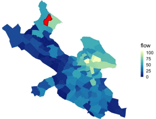
neighborhoods. SeeFig 2for linkage strength values between an example stadsdel and all other stadsdelar.
Relationship with more traditional connectivity metrics. We compare our linkage
strength metric to that used in [15,16], which calculates origin-destination pairs from Twitter data in order to identify commuting patterns and validate travel demand models, respectively. Their metric identifies instances of successive tweets by the same user in two different regions within four hours of one another as an origin-destination trip; flow between two areas is the total number of origin-destination trips between them. They find that the metric performs well in approximating commuting patterns as identified by census survey data and estimated by the SCAG travel demand model. This type of method is infeasible with our dataset, as suc-cessive tweets may occur weeks or months apart and do not necessarily correspond to
origin-Fig 2. Linkage strength between example stadsdel and all other stadsdelar. Color of each stadsdel represents the value of its linkage strength with the stadsdel highlighted in red, where lighter stadsdelar are more strongly connected to the stadsdel in red and darker stadsdelar are more weakly connected. Note that there is strong connection between the example stadsdel and the stadsdelar in the city center of Stockholm—as these central stadsdelar have high levels of Twitter activity in general, they have strong connection to all other stadsdelar—we control for this difference in Twitter activity volume in our model.
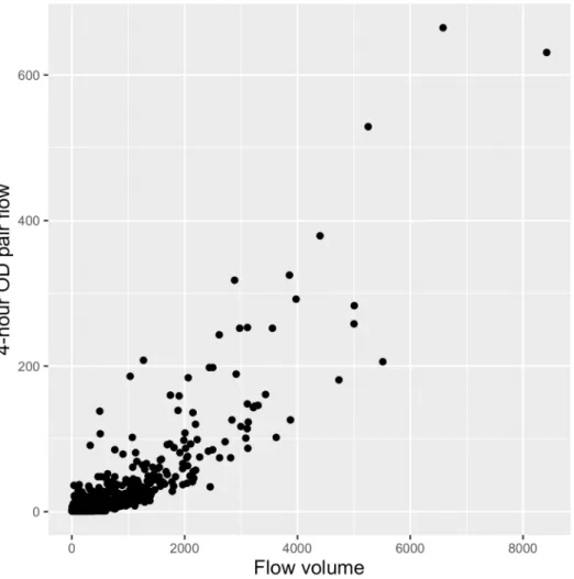
destination pairs; however, we find that our metric is strongly correlated with the metric used in [15,16], (correlation coefficient .85, p-value << 0.001, seeFig 3) while still allowing us to retain the use all of our data—our metric incorporates information from all roughly 280,000 of our tweets, while the origin-destination flow metric would only be able to incorporate infor-mation from 65,521 of those tweets (24,491 OD-pairs).
Privacy concerns. Usernames and text associated with the tweets are dropped from our
dataset. User ids are hashed to new, random values in order to fully anonymize our data. Fur-ther, once linkage strength is calculated, tweets are no longer associated with individuals at all, and trajectories are untraceable in the data. Thus, we remove all identifying information from our data, and we do not add identifying data via home location estimation.
Model
We use a negative binomial regression to estimate the relationship between our explanatory variables (described below) and linkage strength between pairs of stadsdelar. Linkage strength is a count variable, but it is overdispersed with respect to a Poisson distribution (mean = 102.6, variance = 80056.90); negative binomial regression is appropriate for this kind of overdis-persed count data [22]. Because all of our explanatory variables are determined by the origin
Fig 3. Relationship between linkage strength and existing metric. Our linkage strength metric is on the x-axis, flow as measured by origin-destination pairs from which the same user tweeted within four hours on the y-axis. Pearson correlation coefficient is .853, p-value << .001.
stadsdel, the destination stadsdel, or a function of the two, we use clustered standard errors as recommended in [23], where the data is clustered on bothA and B—seeDiscussionfor more details. The geospatial nature of our data suggests there could be potential issues with residual spatial autocorrelation [24]; however, we find no residual spatial autocorrelation in any of our three models (seeS2 Appendix).
In order to understand differences between stadsdelar in the impact of socioeconomic dif-ference on movement patterns, we also estimate individual negative binomial regression mod-els for each stadsdel. We use fewer explanatory variables—the variables related to origin stadsdel (A) are no longer relevant, as we are looking at only pairs with the same origin stads-del, and we remove several highly collinear variables, as they contain redundant information and we have fewer degrees of freedom in these smaller models. SeeTable 1for the full list of explanatory variables used in the individual-stadsel and all-stadsdelar models. We use the GLM module in the statsmodels python package in order to estimate all of our negaitve bino-mial regression models.
Explanatory variables
Variable of interest: Socioeconomic dissimilarity. We examine whether absolute
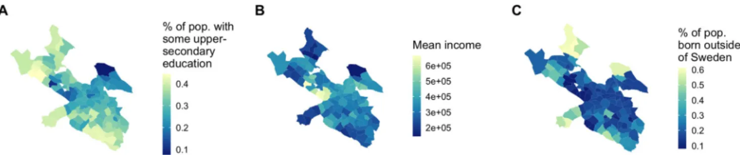
differ-ence in socioeconomic characteristics between two areas affects the linkage strength between them—are neighborhoods more connected by flow of people to other neighborhoods “like” theirs, in terms of mean income, education levels, and immigrant makeup? We choose three socioeconomic variables for each stadsdel: mean income, percentage of the population with some post secondary education, and percentage of the population classified as “first genera-tion” (those born outside of Sweden). These three characteristics are correlated with one another but distinct—seeFig 4. For each of the three socioeconomic attributes, we run a nega-tive binomial regression on all pairs of stadsdelar. The dependent variable is linkage strength between the two stadsdelar and the variable of interest is absolute difference in their socioeco-nomic attributes.
Table 1. Explanatory variables used in individual-stadsdel and all-stadsdel models. Individual stadsdel models All stadsdelar models Variable
✔ ✔ Socioeconomic difference
✔ Transit time
✔ ✔ Driving time
✔ Labor accessibility A
✔ ✔ Labor accessibility B
✔ Log points of interest A
✔ ✔ Log points of interest B
✔ Population A ✔ Population B ✔ ✔ Rank-distance model ✔ Income A ✔ Income B ✔ Education A ✔ Education B ✔ Foreign background A ✔ Foreign background B ✔ Total linkage strength from A
✔ ✔ Total linkage strength from B
Control variables. We look at five control variables that can help to account for travel
constraints and layout of the city: travel time between two locations, physical accessibility of each location in the city structure, number of points of interest in each location, population of each location, and expected linkage strength in a rank-distance null model of mobility.
Travel times. We use the Google Maps API to calculate travel times via driving and public
tran-sit between two areas. As longer travel times indicate that areas are more expensive to travel between in terms of both time and money, we expect an inverse relationship between the travel time between two places and linkage strength between them. Analysis of this travel time data indicates heterogeneities in the strength of the transportation network between different neighborhoods—seeS3 Appendixfor more details.
Accessibility. We use a labor accessibility index based on the SCAPER travel demand model
[17,18]. The index acts as a proxy for the proportion of the city’s population that can access the area during the day subject to constraints imposed by daily schedules, mandatory travel locations (work, school) and travel times, which incorporate road and public transit net-works as well as traffic information; thus, we expect a positive relationship between accessi-bility of an area and linkage strength to that area. SeeS4 Appendixfor more details. The index is reported at the EMME node level, which we aggregate up to the stadsdel level by assigning each stadsdel the average of the accessibility indices attributed to the EMME nodes inside of it.
Points of Interest (POIs). We download information on points of interest in each stadsdel from
OpenStreetMap. Points of interests include shops, restaurants, tourism sites, parks, among other types of places. As points of interest draw visitors to an area, they could help to explain movement around Stockholm. In order to specifically capture points of interest that would indicate attractiveness of an area, we filter out passive POIs which do not serve as a draw to an area, such as trash cans and surveillance cameras—seeS1 Appendixfor full list of POI categories. Existing work has shown that OSM data is highly positionally accurate but incomplete (for example [25], found that only 70% of US schools identified in an authoritative national dataset were mapped in OSM); we assume that level of incomplete-ness is uniform across Stockholm [26].
Population. We use 2017 population counts from the Swedish census (source: City of
Stock-holm municipality’s Statistical Information Service).
Rank-distance null model. We estimate expected travel linkage strengths between areas of
Stockholm using the rank-distance model in [27]. This models movement between two placesA and B as inversely proportional to rankA(B), where rankA(B) is the number of
Fig 4. Socioeconomic variables of interest. (A) Percent of the population with some level of post-secondary education. (B) Mean income. (C) Percent of the population first-generation.
points of interest closer toA than B is to A. In [27], Noulas et al. find the rank-distance model to fit better than other commonly-used models of human movement, such as gravity models, for within-city travel patterns. Estimating expected linkage strength using this model allows us to account for movement between two places that have only to do with the distribution of amenities across Stockholm, helping us to further isolate choice in the rela-tionship between socioeconomic similarity and linkage strength.
We also include total Twitter activity and the individual socioeconomic characteristics of each stadsdel. In summary, the explanatory variables for the individual-stadsdel and all-stads-del moall-stads-dels are reported inTable 1. There do exist some correlations between our dependent variables, but they do not result in severe multicollinearity issues—seeS2 Appendixfor full details.
Since our measure of linkage strength is symmetric, the characteristics of each location should contribute equally to it; for this reason, we fix the coefficients on socioeconomic char-acteristics, accessibility, points of interest, population, total amount of linkage strength and total number of tweets to be the same for both locations (e.g., the coefficient on population of stadsdel A is equal to the coefficient on population of stadsdel B) by including their sums instead of their individual values. We also perform a log transform on accessibility, points of interest, population, and total number of tweets in order to capture the empirical relationship between those variables and our linkage strength metric.
Results
The outcome of our regression analysis is detailed inTable 2. Controlling for covariates, we see that education and income have significant effects on the linkage strength between two regions at the levelα = .001, while foreign background has a signficant effect on linkage strength atα = .1. For every standard deviation increase in socioeconomic difference, we see
Table 2. All-stadsdel model results.
linkage strength between A and B
Income Education Foreign background
Constant 3.528���(0.040) 3.528���(0.040) 3.530���(0.040)
Income difference -0.093���(0.027)
Education difference -0.105���(0.021)
Foreign background difference -0.035�(0.020)
Transit time -0.144���(0.031) -0.138���(0.030) -0.140���(0.031)
Driving time -0.157���(0.023) -0.147���(0.023) -0.163���(0.023)
Log labor accessibility A, log labor accessibility B 0.225���(0.054) 0.235���(0.056) 0.232���(0.056)
Log points of interest A, log points of interest B 0.223���(0.072) 0.223���(0.071) 0.238���(0.070)
Log population A, log population B 0.033 (0.031) 0.030 (0.031) 0.024 (0.031)
Rank-distance model 0.073���(0.041) 0.071���(0.014) 0.075���(0.014)
Income A, income B -0.075�(0.043) -0.126���(0.040) -0.137���(0.042)
Education A, education B -0.077��(0.032) -0.088���(0.032) -0.089���(0.032)
Foreign background A, 0.114���(0.039) 0.114���(0.035) 0.076��(0.038)
Total Twitter activity in A, total Twitter activity in B 0.939���(0.070) 0.937���(0.070) 0.935���(0.070) Note:
�p<0.1; ��p<0.05; ���p<0.01
total linkage strength multiplied by the exponential of the given coefficient; thus, for every standard deviation increase in income difference between A and B (85,525.27 Swedish krona, equivalent to around 10,251 USD), linkage strength between A and B is multiplied bye−0.097= .91, leading to a 8.9% decrease in linkage strength between A and B. For every standard deviation increase in post-secondary education difference between A and B, we see a 10.0% decrease in linkage strength between A and B. For every standard deviation increase in immigrant makeup difference between A and B, we see a 3.4% decrease in link-age strength between A and B. Socioeconomic differences between neighborhoods thus pro-duce statistically significant barriers to linkage strength throughout the city—in the case of income and education, quite stark barriers; in the case of immigration status, relatively weaker barriers.
Importantly, driving and transit time are also significant predictors of linkage strength, and have even larger effects than socioeconomic difference—longer travel times by either mode of transportation are associated with significantly less linkage strength. This indicates that each serves a separate and significant role in connecting physical locations in the city. Strengthening physical infrastructure between parts of the city with low linkage strength could similarly serve to strengthen connectivity between dissimilar places: our results suggest that a decrease of one standard deviation in transit time (about fourteen minutes) is associated with about a 13.4% increase in linkage strength between two stadsdelar.
Individual-stadsdel models
We find that predictive effect of socioeconomic difference varies by stadsdel, and is even insig-nificant in some. In most stadsdelar where socioeconomic difference does have a siginsig-nificant predictive effect on linkage strength, that effect is negative, indicating that neighborhoods are more likely to be connected to other neighborhoods with a similar socioeconomic makeup, consistent with our full-city model. However, there is also a significantly positive effect in some stadsdelar—some neighborhoods are significantly more likely to be connected to neigh-borhoods which are different from them, contrary to the overall trend in Stockholm (seeFig 5).Fig 6shows the size of the effect in stadsdelar where it is significant (stadsdelar with no sig-nificant effect are shown in gray). As in the all-stadsdel models, the homophily effect is weakest in the foreign background models—education and income seem to have a much stronger effect on connection between stadsdelar.
Fig 5. Histograms of individual stadsdel model coefficients. Histogram of coefficients on education (A), income (B), and foreign background (C) difference in individual statsdelar models. In the individual-stadsdel income and education models, more negative coefficients are statistically significant at thep < 0.5 level and there are larger negative coefficients than positive ones, which is consistent with the overall trend of a negative relationship between socioeconomic difference and linkage strength. However, this trend is less clear in the foreign background models.
Discussion
We have identified significantly stronger linkage between neighborhoods of similar income, education levels, and immigrant makeup. This relationship persists even when controlling for factors induced by the structure and layout of the city, such as transit time between places and intervening opportunities, indicating some level of homophily in the way that individuals choose to move through neighborhoods. This lack of linkage strength between neighborhoods with different socioeconomic characteristics has important implications for social segregation in Stockholm. Researchers have already identified strong residential segregation between eth-nic Swedes and immigrants to Sweden and between socioeconomic groups [6]; our results sug-gest that this segregation persists in activity spaces as well. Further, our results seem to sugsug-gest that while difference in immigrant makeup does have a significant effect on connectivity between two stadsdel, it is a small one in comparison to the effects of income and education level. The strong immigrant/non-immigrant residential segregation identified in [6] may weaken as Stockholm residents move through daily activity spaces.
Policymakers have already instituted various policies to try to ameliorate residential divides. For example, the Swedish Migration Agency discourages new immigrants to the city from liv-ing in certain socioeconomically challenged neighborhoods by withholdliv-ing some state benefits if they choose to do so [28]. The neighborhoods in Stockholm specifically that are included in this provision—parts of Rinkeby, Husby, and Tensta—have some of the strongest income, educationand foreign background dissimilarity coefficients in Stockholm, suggesting that
they aren’t well connected to the rest of the city in terms of linkage strength; our results suggest that encouraging new migrants to move elsewhere could potentially have the desired effect of faster integration into Sweden in that they may be more likely to be exposed to people from all across the city [29]. However, our results also suggest that socioeconomically similar commu-nities are connected to one another regardless of physical proximity and accessibility, implying that residential integration alone may not be enough to break down social barriers in Stock-holm. Creating public spaces or mixed-income housing units that link areas of different income and education level or immigration background could help to break down existing limits to city connectivity beyond residential segregation.
In our individual-stadsdel models, we have found heterogeneities in the effect of socioeco-nomic dissimilarity on city connectivity across neighborhoods: consistent with the overall model, most significant socioeconomic difference coefficients in the income and education models were negative, but there were still some stadsdelar with significant, positive coeffi-cients, indicating that they are more likley to be strongly connected to stadsdlardifferent from
them by the flow of people. Using the individual-stadsdel models, we were able to identify which stadsdelar have the most significant homophily effect. These stadsdelar could potentially
Fig 6. Individual model coefficients. Socioeconomic difference coefficients in the individual-stadsdel education (A), income (B), and foreign background (C) models. Transparent stadsdelar have statistically insignificant coefficients at the .05 level.
be areas of interest for Stockholm city planners as they plan for activities and spaces that will foster integration.
While the results are promising, it is important that we recognize potential biases in the Twitter data used in this study. Direct demographic information of Twitter users are not avail-able, but language processing studies and formal surveys have found that Twitter’s user popu-lation is, in general, younger, more educated, and wealthier than the general popupopu-lation [30, 31]. Further, while geotagged Tweets can serve as a proxy for user location [32], they are not ground-truth: Twitter users opt in to location-sharing, so they may not share the location of every tweet they send and they most likely do not tweet from every location they go to. Selec-tion biases come from both layers of this—the locaSelec-tions that users choose to report may not be representative of their full distribution of tweeting locations, and the locations from which users tweet may not be representative of their full travel trajectories. That being said [33], com-pares an analysis of six million geotagged tweets across Australia to existing analyses of call data records (which do not contain the previously discussed Twitter biases) to find that Twitter data is, in fact, a useful proxy for human mobility. Their analysis suggests that any biases in our Twitter data may have only limited impact on the results. Future work replicating our findings with, for instance, call detail records from distinct operators [34] could shed more light on this. Finally, Twitter data is known be dominated by certain users, with a small subset of users producing the majority of tweets [30]. In order to ensure that our results are not sensi-tive to a few, highly influential users, we repeated our analysis with the additional constraint that we filtered out repeated tweets from the same user in a given stadsdel on a given day, ensuring that high-volume users are not over-represented in the data (a process similar to that in [35]). This analysis produced no major changes in the fitted coefficients of our models—see S1 Appendixfor full results.
Our distance calculations pose a further limitation to our analysis—travel times were calcu-lated using the geographic centroid of each stadsdel, which may not be representative of travel times between all points in the stadsdelar. Further research could help to illuminate exactly what biases arise from this, if any (see [36]).
Our data is cross-classified and multilevel in structure: each observationfA,Bbelongs to a
cluster of observations associated with stadsdelA and a cluster of observations associated with
stadsdelB. The natural statistical dependencies that will occur in data of this structure are
known to cause deflated standard errors and thus over-rejection of the null hypothesis. We choose to account for this using clustered standard errors as recommended in [23], where the data is clustered on bothA and B. While strategies such as multilevel modeling have been
shown to be even more effective at reducing over-rejection of the null hypothesis than cluster-adjusted standard errors, we believe that a single level model is sufficient and preferable in our context due to its simplicity and interpretability [37]. It should be noted that our data’s cross-classified structure may cause bias in coefficients on level 2 variables (variables associated with an individual stadsdel); however, we do not attempt to interpret any level 2 variables in this case [38].
It is worth exploring more deeply the causal mechanisms behind the lack of connection between dissimilar places that is demonstrated by our results. Specifically, analyzing the rela-tionship between flow of people between places and infrastructure allowing for that flow (e.g., public transit and road networks) could have important implications for urban design, trans-portation planning, and the efficient orchestration of network slices. Using place-based mea-sures like ours as opposed to person-based meamea-sures is especially amenable to this kind of analysis and planning, as they allow for the identification of weak spots in connectivity of the physical environment, as opposed to other measures of social segregation which look at lack of connectivity in social networks—a metric agnostic of the physical environment.
Supporting information
S1 Appendix. Data pre-processing. We discuss the cleaning process of our Twitter and point
of interest data. (PDF)
S2 Appendix. Verification of certain model assumptions. We show that our model does not
suffer significantly from bias related to residual spatial autocorrelation or multicollinearity. (PDF)
S3 Appendix. Travel time data. We describe the travel time data used in our model.
(PDF)
S4 Appendix. Labor accessibility index. We describe the labor accessibility index used in our
model and show how it is distributed across the city of Stockholm. (PDF)
Acknowledgments
The authors would like to acknowledge the Senseable Stockholm Lab and its partners: City of Stockholm, KTH Royal Institute of Technology, the Stockholm Chamber of Commerce and Newsec, in collaboration with MIT Senseable City Lab. We would also like to acknowl-edge the H2020 5G-TOURS project. Finally, we would like to thank the City of Stockholm municipality’s Statistical Information Service for provision of population counts and socio-economic data.
Author Contributions
Conceptualization: Cate Heine, Cristina Marquez, Paolo Santi, Carlo Ratti. Data curation: Cate Heine, Cristina Marquez, Paolo Santi, Marcus Sundberg. Formal analysis: Cate Heine.
Methodology: Cate Heine, Cristina Marquez, Paolo Santi, Carlo Ratti. Supervision: Paolo Santi, Carlo Ratti.
Visualization: Cate Heine, Cristina Marquez.
Writing – original draft: Cate Heine, Cristina Marquez, Paolo Santi, Marcus Sundberg. Writing – review & editing: Cate Heine, Cristina Marquez, Paolo Santi, Marcus Sundberg,
Miriam Nordfors.
References
1. Bureau USC. Metropolitan and Micropolitan About; 2015. Available from:https://www.census.gov/ programs-surveys/metro-micro/about.html.
2. Bettencourt L. The Origins of Scaling in Cities. Science (New York, NY). 2013; 340:1438–1441.https:// doi.org/10.1126/science.1235823
3. Bora N, Chang YH, Maheswaran R. Mobility patterns and user dynamics in racially segregated geogra-phies of US cities. In: International Conference on Social Computing, Behavioral-Cultural Modeling, and Prediction. Springer; 2014. p. 11–18.
4. Wang Q, Phillips NE, Small ML, Sampson RJ. Urban mobility and neighborhood isolation in America’s 50 largest cities. Proceedings of the National Academy of Sciences of the United States of America. 2018; 115(30):7735–7740.https://doi.org/10.1073/pnas.1802537115PMID:29987019
5. Xu Y, Belyi A, Santi P, Ratti C. Quantifying segregation in an integrated urban physical-social space. Journal of the Royal Society Interface. 2019; 16(160).https://doi.org/10.1098/rsif.2019.0536 6. Rokem J, Vaughan L. Geographies of ethnic segregation in Stockholm: The role of mobility and
co-presence in shaping the ‘diverse’ city. Urban Studies. 2019; 56(12):2426–2446.https://doi.org/10.1177/ 0042098018795561
7. Prestby T, App J, Kang Y, Gao S. Understanding neighborhood isolation through spatial interaction net-work analysis using location big data. Environment and Planning A: Economy and Space. 2020; 52 (6):1027–1031.https://doi.org/10.1177/0308518X19891911
8. Dorman M, Svoray T, Kloog I. How does socio-economic and demographic dissimilarity determine physical and virtual segregation? Journal of Spatial Information Science. 2020; 21(21).https://doi.org/ 10.5311/JOSIS.2020.21.587
9. Zhang W, Thill JC. Detecting and visualizing cohesive activity-travel patterns: A network analysis approach. Computers, Environment and Urban Systems. 2017; 66:117–129.https://doi.org/10.1016/j. compenvurbsys.2017.08.004
10. Zhang M, Zhang W, Pang H, et al. Identifying the local and regional travel effects of activity centers in the Austin, Texas area. Southwest Region University Transportation Center (US); 2015.
11. Browning CR, Calder CA, Krivo LJ, Smith AL, Boettner B. Socioeconomic segregation of activity spaces in urban neighborhoods: Does shared residence mean shared routines? The Russell Sage Foundation Journal of the Social Sciences (RSF). 2017; 3(2):210–231.
12. Li F, Wang D. Measuring urban segregation based on individuals’ daily activity patterns: A multidimen-sional approach. Environment and Planning A. 2017; 49(2):467–486.https://doi.org/10.1177/ 0308518X16673213
13. Zhang W, Thill JC. Mesoscale Structures in World City Networks. Annals of the American Association of Geographers. 2019; 109(3):887–908.https://doi.org/10.1080/24694452.2018.1484684
14. Longley PA, Adnan M. Geo-temporal Twitter demographics. International Journal of Geographical Infor-mation Science. 2016; 30(2):369–389.https://doi.org/10.1080/13658816.2015.1089441
15. Gao S, Yang J, Yan B, Hu Y, Janowicz K, McKenzie G. Detecting Origin-Destination Mobility Flows From Geotagged Tweets in Greater Los Angeles Area. Eighth International Conference on Geographic Information Science (GIScience 2014). 2014; p. 0–4.
16. Lee JH, Gao S, Goulias K. Can Twitter data be used to validate travel demand models? In: Proceedings of the 14th International Conference on Travel Behaviour Research (ICTBR 2015). Windsor, UK; 2015.
17. Jonsson D, Karlstro¨ m A, Oshyani MF, Olsson P. Reconciling User Benefit and Time-Geography-Based Individual Accessibility Measures. Environment and Planning B: Planning and Design. 2014; 41 (6):1031–1043.https://doi.org/10.1068/b130069p
18. Va¨stberg OB, Karlstro¨ m A, Jonsson D, Sundberg M. A dynamic discrete choice activity-based travel demand model. Transportation Science. 2020; 54(1):21–41.
19. Marquez C, Gramaglia M, Fiore M, Banchs A, Ziemlicki C, Smoreda Z. Not All Apps Are Created Equal: Analysis of Spatiotemporal Heterogeneity in Nationwide Mobile Service Usage. In: Proceedings of the 13th International Conference on Emerging Networking EXperiments and Technologies (ACM CoNEXT 2017). Incheon, Republic of Korea; 2017. p. 180–186.
20. Huang Q, Wong DWS. Activity patterns, socioeconomic status and urban spatial structure: what can social media data tell us? International Journal of Geographical Information Science. 2016; 30(9):1873– 1898.
21. van Eggermond MAB, Chen H, Erath A, Cebrian M. Investigating the potential of social network data for transport demand models; 2015. Transportation Research Board 95th Annual Meeting, United States.
22. Hilbe JM. Negative Binomial Regression. 2nd ed. Cambridge University Press; 2011.
23. Abadie A, Athey S, Imbens GW, Wooldridge J. When Should You Adjust Standard Errors for Cluster-ing? National Bureau of Economic Research; 2017. 24003.
24. Fotheringham AS. The Problem of Spatial Autocorrelation and Local Spatial Statistics. Geographical Analysis. 2009; 41(4):398–403.https://doi.org/10.1111/j.1538-4632.2009.00767.x
25. Jackson SP, Mullen W, Agouris P, Crooks A, Croitoru A, Stefanidis A. Assessing completeness and spatial error of features in volunteered geographic information. ISPRS International Journal of Geo-Information. 2013; 2(2):507–530.https://doi.org/10.3390/ijgi2020507
26. El-Ashmawy KLA. Testing the positional accuracy of OpenStreetMap data for mapping applications. Geodesy and Cartography. 2016; 42(1):25–30.https://doi.org/10.3846/20296991.2015.1160493 27. Noulas A, Scellato S, Lambiotte R, Pontil M, Mascolo C. A tale of many cities: Universal patterns in
human urban mobility. PLoS ONE. 2012; 7(5).https://doi.org/10.1371/journal.pone.0037027PMID:
28. Your own accommodation; 2020. Available from: https://www.migrationsverket.se/English/Private-individuals/Protection-and-asylum-in-Sweden/While-you-are-waiting-for-a-decision/Accommodation/ Your-own-accommodation.html.
29. Areas that may affect the right to compensation for asylum seekers; 2020. Available from:https://www. migrationsverket.se/English/Private-individuals/Protection-and-asylum-in-Sweden/While-you-are- waiting-for-a-decision/Accommodation/Your-own-accommodation/Areas-that-may-affect-the-right-to-compensation-for-asylum-seekers.html.
30. Wojcik S, Hughes A. Sizing Up Twitter Users; 2019. Available from:https://www.pewresearch.org/ internet/2019/04/24/sizing-up-twitter-users/.
31. Longley PA, Adnan M, Lansley G. The geotemporal demographics of twitter usage. Environment and Planning A. 2015; 47(2):465–484.https://doi.org/10.1068/a130122p
32. Hawelka B, Sitko I, Beinat E, Sobolevsky S, Kazakopoulos P, Ratti C. Geo-located Twitter as proxy for global mobility patterns. Cartography and Geographic Information Science. 2014; 41(3):260–271.
https://doi.org/10.1080/15230406.2014.890072
33. Jurdak R, Zhao K, Liu J, Abou Jaoude M, Cameron M, Newth D. Understanding Human Mobility from Twitter. PLoS ONE. 2015; 10.
34. Moyano A, Moya-Go´mez B, Gutie´rrez J. Access and egress times to high-speed rail stations: a spatio-temporal accessibility analysis. Journal of Transport Geography. 2018; 73:84–93.https://doi.org/10. 1016/j.jtrangeo.2018.10.010
35. Gao S, Janowicz K, Montello DR, Hu Y, Yang JA, McKenzie G, et al. A data-synthesis-driven method for detecting and extracting vague cognitive regions. International Journal of Geographical Information Science. 2017; 31(6):1245–1271.
36. Jiang Y, Li Z, Ye X. Understanding demographic and socioeconomic biases of geotagged Twitter users at the county level. Cartography and Geographic Information Science. 2019; 46(3):228–242.https://doi. org/10.1080/15230406.2018.1434834
37. Cheah BC. Clustering standard errors or modeling multilevel data. University of Columbia. 2009; p. 2–4.
38. Johnson BD. Cross-Classified Multilevel Models: An Application to the Criminal Case Processing of Indicted Terrorists. Journal of Quantitative Criminology. 2012; 28(1):163–189.https://doi.org/10.1007/ s10940-011-9157-3