Automated fault detection without seismic processing

Automated fault detection without seismic processing

The MIT Faculty has made this article openly available.

Please share

how this access benefits you. Your story matters.

Citation

Araya-Polo, Mauricio, Taylor Dahlke, Charlie Frogner, Chiyuan

Zhang, Tomaso Poggio, and Detlef Hohl. “Automated Fault Detection

Without Seismic Processing.” The Leading Edge 36, no. 3 (March

2017): 208–214 © 2017 Society of Exploration Geophysicists

As Published

http://dx.doi.org/10.1190/tle36030208.1

Publisher

Society of Exploration Geophysicists

Version

Final published version

Citable link

http://hdl.handle.net/1721.1/110058

Terms of Use

Article is made available in accordance with the publisher's

policy and may be subject to US copyright law. Please refer to the

publisher's site for terms of use.

Automated fault detection without seismic processing

Abstract

For hydrocarbon exploration, large volumes of data are acquired and used in physical modeling-based workflows to identify geologic features of interest such as fault networks, salt bodies, or, in general, elements of petroleum systems. The adjoint modeling step, which transforms the data into the model space, and subsequent interpretation can be very expensive, both in terms of computing resources and domain-expert time. We propose and implement a unique approach that bypasses these demanding steps, directly assisting interpretation. We do this by training a deep neural network to learn a mapping relationship between the data space and the final output (particularly, spatial points indicating fault presence). The key to obtaining accurate predictions is the use of the Wasserstein loss function, which properly handles the structured output — in our case, by exploit-ing fault surface continuity. The promisexploit-ing results shown here for synthetic data demonstrate a new way of using seismic data and suggest more direct methods to identify key elements in the subsurface.

Introduction

Acquisition technology advances and exploration of complex areas are pushing the amount of data to be analyzed into the “big data” category. Current exploration workflows consist of many partially automated steps in which domain experts (geolo-gists, geophysicists, rock physicists, etc.) command highly tuned applications and then curate the resulting data in search of valuable information. The data explosion is stressing these workflows to a point at which every year more of the data remains unused. Generally, the exploration process can be broken down into two main elements: advanced tools and manpower. Tools have progressed, and the addition of high-performance computing has helped to reduce turnaround times for seismic imaging (Rubio et al., 2009; Rastogi, 2011). Even in the extreme case in which execution time for processing tools would take nearly zero time, the problem of manpower remains; there is no sensible way in which domain experts can analyze and interpret all incoming data. The best solution must trade domain-expert time for computing time. Therefore, some of that domain knowledge needs to be formalized and imple-mented within existing and future tools. One way to achieve this is by taking advantage of algorithms that learn, for instance, from legacy data that have been properly vetted. Using machine learning, we can take advantage of new algorithms and software ecosystems, as well as specialized hardware. In this contribu-tion, we will focus our attention on one such application of machine learning.

Seismic imaging is the primary tool used to build high-res-olution models of the subsurface. In practice, it is typically part

Mauricio Araya-Polo

_{, Taylor Dahlke}

_{, Charlie Frogner}

_{, Chiyuan Zhang}

_{, Tomaso Poggio}

_{, and Detlef Hohl}

of an iterative workflow that alternates between imaging steps and model update steps. This iterative refinement is expensive in terms of human costs (picking out features/adjusting the velocity model) and computational costs (many repeated wave propagations and attributes computations). Most prior work focused on identify-ing features in already migrated images (Hale, 2012; Hale, 2013; Guillen, 2015; Addison, 2016; Bougher and Hermann, 2016). The literature is filled with refinements to this workflow, but ultimately, it remains largely the same.

Recent work (Zhang et al., 2014; Frogner et al., 2015; Dahlke et al., 2016) demonstrates a new approach that builds and uses a deep neural network (DNN) statistical model to transform raw-input seismic data directly to the final mapping of faults in 2D. In this case, fault locations were chosen as the output because of their relevance to optimizing production in existing fields. DNNs are built on the premise that they can be used to replicate any function (in theory, even a nonlinear one like acoustic wave propagation). We show that DNNs can be used to identify fault structure in 3D volumes with reasonable accuracy. The greater promise is that as computational tools improve, we can use even more complex neural networks to improve accuracy. The costs are all computational, mostly in the form of training incurred only once up front. Once the neural network is trained, predictions can be produced in a fraction of the training time and of the time needed for tradi-tional physics modeling with partial differential equations. This means that nearly instantaneous earth models could be created as acquisition progresses. An interpreter aboard an acquisition vessel could identify hot spots as they travel over them and then modify acquisition to improve imaging over that same area on another pass. This is more cost effective than initiating a new acquisition campaign.

In this paper, we start by explaining the basics of the problem followed by discussions of DNNs and the Wasserstein loss func-tion. Next, we introduce the general workflow used to train our DNN. After that, we discuss our performance results and some of our findings regarding network architectural parameters. Last, we will explain the directions for future work.

Problem overview

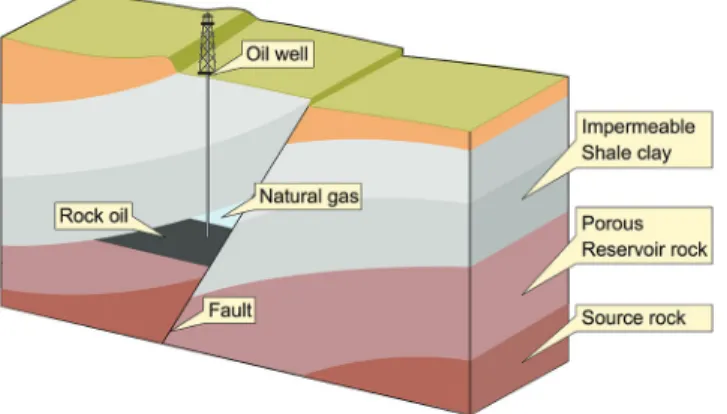
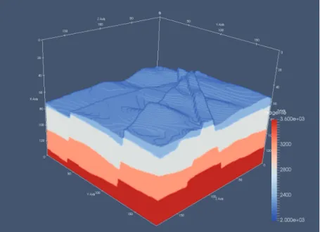
The key geologic feature we target in this work is a fault network. Shifted rock layers can trap liquid hydrocarbons, which will form reservoirs (Figure 1). The 3D structure of a fault network can be highly complex (Figure 2), representing a challenge for structured output methods of prediction.

Deep neural networks (DNN)

Using learning algorithms is an appealing alternative to classic seismic processing. Among that class of algorithms, we have

1_{Shell International Exploration and Production Inc.} 2_{Stanford University.}

3_{Massachusetts Institute of Technology.}

http://dx.doi.org/10.1190/tle36030208.1.

selected DNN for our experiments since there is increasing com-munity agreement (Grzeszczuk et al., 1998; De et al., 2011; Lin and Tegmark, 2016) in favor of this kind of algorithm as a good surrogate for physics-based processes.

DNNs consist of “layers” of weighted nodes that are activated by inputs from previous layers. These networks are trained with examples in which the correct/true output (label) is known for a given input; the weight parameters in the nodes of the network evolve due to the minimization of the error between prediction and true value. This causes the network to become an increasingly better predictor of the training examples and, ultimately, of any example (assuming proper training) of a data class that is similar in nature to the training data.

This topology of information flow between nodes is inspired by the structure of neurons in the brain (Figure 3). The universal approximation theorem shows that neural networks can be used to approximate an arbitrary continuous function up to our desired accuracy (Hornik et al., 1989). For this reason, there is much promise in using this approach to make predictions of functions that are very nonlinear (like fault probability from time-series data). While the theoretical limits of this approach are generous, to find the neural network that best approximates our function is not trivial. Our ability to build effective neural networks is limited by computing constraints. More complex networks are more expensive to train, and the generation of accurate training examples can be computationally expensive due to large-scale forward modeling. Ultimately, our predictions are only as good as the complexity and refinement of our neural network coupled with the relevance and quality of the features we choose as inputs.

Workflow

The first step in our workflow (Figure 4) is to collect the training examples. Real data examples are impractical and limiting since the labels are assigned to fault locations by few domain experts. This means that the neural network’s best result would be bound by human performance and data quality. Instead, we generate realistic 3D velocity models synthetically, with the fault labeling generated concurrently for an unbiased ground truth. Next, we use an acoustic approximation to the wave equation to generate wavefields and record them as time-series signals with predefined acquisition geometry. This step is conducted on thousands of random velocity-model realizations, giving us many instances of labeled fault locations and the corresponding seismic traces for the entire data set. We reserve a portion of this data set unseen from the algorithm (holdout set) so that we can test it after we have trained our predictor. We set ranges on a relatively small number of parameters as bounds on the random model generator. These parameters include the number of layers in a model, the number of faults, the range of velocity, and the dip and strike angles for each possible fault. We believe that the randomized models pro-duced in this manner are realistic enough to demonstrate the efficacy of neural network predictions (see Figure 5).

Labeling

Since the positions of the faults are known a priori, the labeling process is straightforward. However, complexity is added to this process when the labeling targets a subsampled grid for compu-tational efficiency. Addition of a threshold parameter to define the labeling of the coarse grid is needed. This threshold value sets how many fine-sampled voxels inside a coarse voxel must be fault-labeled for that coarse voxel to be considered as having a fault or not. There are a variety of ways to choose that threshold

Figure 1. Diagram of a fault trap (Creative Commons).

Figure 2. Example of complex faulting (from Mira Geoscience).

Figure 3: Topology of a simple neural network.

Figure 4. Depiction of the workflow’s main tasks.

so that the subsampled labeling appropriately matches the underlying fine-sampled labeling, with ours being chosen on a trial-and-error basis prior to any training.

Structured output learning and the

Wasserstein loss

Our problem is naturally formulated as pre-dicting a (subsampled) 3D “voxel map” of binary fault/nonfault indicators. This is similar to image segmentation problems in computer vision. A common way of handling this is to introduce a Markov random field (MRF) on the output voxels that captures the interactions and run an inference algorithm to get the jointly optimal predictions. More generally, the inference step can be incor-porated into the objective function for learning. Commonly used formulations include structured support vector machines and conditional random fields (Nowozin and Lampert, 2011).

However, while the couplings for pixel labels in an image can be modeled naturally via

neigh-borhood similarity or input-pixel-based similarity, the prior structure in our model is of much higher complexity. More specifi-cally, the faults usually extend as smooth surfaces. This property cannot be characterized via factors that involve only a few nearby output variables. On the other hand, inference on MRFs with general high-order factors is computationally expensive. As a result, we choose to perform independent predictions for each output region and incorporate our prior knowledge via a novel loss function called the Wasserstein loss (Frogner et al., 2015).

Formally, let K = D × D × D be the number of output voxels. We normalize the ground-truth binary output vector y ∈ 0,1

{ }

to y = y / y ₁ so that it represents a probability distribution over the 3D grid. Moreover, we model our predictor as a DNN with a softmax layer at the top so that it also produces a probability distribution

h

( )

x

∈ Δ

The cross-entropy loss is commonly used to measure the difference between two distributions. It is derived from the Kull-back–Leibler divergence between the predictionˆy and the ground-truth y : ℓCE

(

)

∑

When the ground-truth y is a “one-hot” vector for a single class, this reduces to the cross-entropy loss typically used in multiclass logistic regression. Unfortunately, this loss does not consider the structural information for the fault-prediction prob-lems. Specifically, the spatial relationship among the K output voxels could enforce strong smoothness information. Consider a prediction that is slightly off the ground truth and another that is completely wrong; the cross-entropy loss cannot effectively distinguish the two different cases.

Alternatively, consider the following Wasserstein loss (Frogner et al., 2015), which is inspired by optimal transport literature and related to other applications on geosciences (Engquist and Froese, 2014; Metivier et al., 2016):

ℓ_W

(

)

Π

₍

₎

{

}

₍

₎

(

)

( )

the output space. For our application, the output space is the 3D grid of voxels, and the natural ground metric is the Euclidean distance between the voxels. T in the loss term is a joint probability distribution that marginalizes to the ground truth and the predic-tion. Intuitively, T defines a transportation plan that maps prob-ability mass from the prediction to the ground-truth, and T ,M

measures the cost of this plan according to the ground metric. The loss is then defined by the cost of the optimal feasible transport plan. For the cases of Figure 7, the Wasserstein loss for the left plot will be smaller than the central plot due to the larger cost of this plan according to the ground metric.

Feature generation and extraction

Raw seismic data is far too unrefined and redundant to be immediately useful as inputs to our neural network. We im-proved prediction performance by extracting input features carefully, taking advantage of techniques from signal processing. The amount of collected features is large and grows by orders of magnitude when more realistic models are used. For instance, for all cases used in this work, the acquisition configuration is: nine shots per model, with 400 receivers in a 20 × 20 grid, and 1500 time samples per receiver. This configuration (smaller than realistic acquisitions) produces 5,400,000 raw features in total per model. If we were to use a more realistic acquisition, such as 100 shots with 1600 receivers and 2000 time samples, we would end up with up to 320,000,000 input attributes. These numbers only grow with denser acquisition geometries. Figure 5. Example of a randomly generated velocity model with a multiple faults.

Choosing the architectural parameters of a neural network is not a deterministic process. A neural network that learns from this amount of features requires a large number of training epochs to train.

We use transformations of the data space coupled with feature-reduction methods for removing the features that are the least useful for prediction. These steps reduce the feature space to a more reasonable magnitude (thousands of input features rather than millions).

Implementation and results

In terms of computing, the training process takes a few hours per data set and minutes for testing. Putting this in perspective, the training process for one data set takes the same time that the migration of a single shot takes for a dense acquisi-tion with anisotropic assumpacquisi-tion. Once the network is trained, it can be reused many times with minimal cost, and given a certain generalization level, it can be exposed to many new data sets. This can be far less expensive than processing and interpret-ing one complete seismic acquisition, which happens every time the underlying model is changed. Our proprietary workflow is almost completely implemented in the MIT Julia language in which the heavy computing is offloaded to GPGPUs through NVIDIA’s CuDNN.

We generate thousands of random velocity models with up to four faults in them, of varying strike, dip angle, and position. Our models had between three and six layers each, with velocities varying from 2000 to 4000 [m/s], with layer velocity increasing with depth. These models were 140 × 180 × 180 grid points at the sampling used for wave propagation (using the acquisition geom-etry described earlier) but were subsampled to 20 × 20 × 20 and 32 × 32 × 32 for labeling purposes. The raw data collected was reduced aggressively to a feature set that can fit in an NVIDIA K80 GPGPU memory.

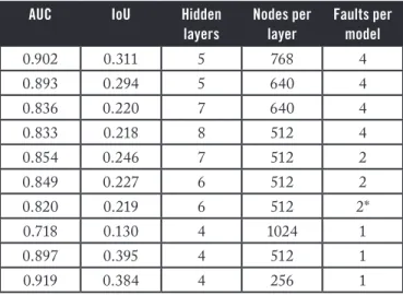
With the generated features and labels, a variety of fully connected deep neural networks are trained. The network architecture main parameters varied from two to 20 hidden layers and 256 to 2048 units per layer. For all cases presented in Table 1, we used the Wasserstein loss function for training. The output of the networks is a subsampled 3D voxel grid, with each voxel’s value indicating the likelihood of a fault being present within the voxel. Ground-truth labels on the same grid were binary valued, indicating presence or not of a fault in each voxel. The final predictions were generated by taking the likelihood values map output and applying a threshold to it, such that likelihood values above the threshold would be considered having a fault, while those below would not. As a result, a lower threshold will label more voxels as faults, while a high threshold labels less.

We use two different quantitative metrics of performance in this work: intersection over union (IoU) and area under the ROC curve (AUC).

The IoU value is a ratio of the number of voxels that are in the intersection of the ground truth and prediction, divided by the number of voxels in the union of the ground truth and prediction. This gives us an idea of how clustered or scattered a prediction is; the values range from 0 to 1, where higher values are better (example in Figure 6). Two predictions could theoretically have the same AUC value (see Table 1) but Figure 6. Comparison of (a) the Wasserstein- and (b) non-Wasserstein-based

predictions, IoU metric (described in the article). Red areas show false positives, green shows true positives (correct predictions), and yellow shows false negative. (c) 2D slice of a 3D model. The predictions have very different IoU, where green means better.

Figure 7. ROC curves for representative DNN architectures. The closer to the top-left corner the better.

Table 1. Results obtained on several representative sets of simulated test data. The first two columns report performance metrics; the other columns describe the parameter of the experiments. All results obtained using Wasserstein loss function, with 16,000 training models and 4000 testing models, except for the asterisked case, where only 10,000 training models and 2000 testing models were used.

AUC IoU Hidden

layers Nodes per layer Faults per model 0.902 0.311 5 768 4 0.893 0.294 5 640 4 0.836 0.220 7 640 4 0.833 0.218 8 512 4 0.854 0.246 7 512 2 0.849 0.227 6 512 2 0.820 0.219 6 512 2* 0.718 0.130 4 1024 1 0.897 0.395 4 512 1 0.919 0.384 4 256 1

different IoU values. We report the (IoU) value averaged for the entire test set of predictions, with predicted likelihoods thresholded at a value chosen to maximize the average IoU over all the predictions.

Each point of a receiver operating characteristics (ROC) curve (see Figure 7) is based on the number of true positive predictions (vertical axis) and the false positive predictions (horizontal axis) for a particular threshold value. We report the AUC for the predictions, which describes how strong our predic-tor is. The value ranges from 0.5 to 1.0, where the higher the value the better.

In Table 1, for all data sets (one, two, and four faults in model) AUC exceeds 0.9, which approaches that needed for practical use. Also, IoU surpasses 0.3 for many experiments, which implies that the prediction can be improved in terms of spatial alignment with respect to the ground truth.

The prediction grid size of experiments in Figure 9 and Figure 11 is 32 × 32 × 32, therefore each prediction represents a voxel of 4 × 5 × 5 in the model space. The predictions in Figure 9 follow the expected results, plus some false positives in the bottom-right area of the back slice.

The predictions in Figure 11b follow the expected structure as can be seen in Figure 11a. However, false positives are present in the area where the faults coincide. This is in line with expecta-tions, since a cornucopia of signals and patterns are produced in that area. This case exposes the current limit of our predicting resolution for complex cases. In general, the resolution is limited by the quality of the data.

Future work

To evaluate practical usability, we must address how this approach can be scaled to actual production-level seismic data sets. For instance, we have to analyze sensitivity of the predic-tions to acquisition geometries. Current synthetic input data is based on fixed acquisition geometry. If we use this fixed geometry to train a predictor, one must bin and stack the ac-quired data so that it matches the acquisition used for training the model. For this reason, we believe that using a fixed dense geometry permits us to accurately bin and stack real data to match the predictor’s input parameters. Denser acquisition means more features, and as a result, more dramatic reduction of the feature space (and/or more complex neural networks) is needed.

Another area where we can improve the prediction quality is by increasing the number of voxels in our downsampled output grid such that we have better resolution in our predictions. This increase in voxel granularity means a more computationally de-manding neural network and thus an increase in the cost of tuning and training.

Our workflow is flexible with respect to what can be predicted. The workflow can be repurposed to build one that predicts, for instance, salt bodies instead of fault locations. We change our labeling scheme so that salt bodies are labeled before training. Since salt bodies often create strong signals (at least for the top-of-salt events) we expect that this geologic feature could also be identified using this method. Preliminary results along this line are promising.

Figure 8. Example of 3D model with two 2D highlighted slices. In this top view, two faults can be identified.

Figure 9. (a) Expected predictions for fault network in Figure 8 velocity model slices. (b) Our DDN-based predictions.

Figure 11. (a) Expected predictions for fault network in Figure 10 velocity model, overlaid on the top view of the model. (b) Our DNN-based predictions.

Figure 10. Random generated 3D velocity model. Top view. A network of four faults can be observed.

Conclusions

We present a novel approach to the challenging multistep seismic model-building problem. It uses a deep learning system to map out a fault network in the subsurface, using raw seismic recordings as input. A distinguishing aspect of the solution is the use of the Wasserstein loss function, which is suited to problems in which the outputs have spatial layout dependency. We dem-onstrate the system’s performance on synthetic data sets with simple fault networks. The primary challenge going forward will be transitioning to fault networks with more complex 3D geometry. This will lead to more tuned existing networks and/or extensions to our workflows.

The application of machine learning approaches to seismic imaging and interpretation shows great promise in hydrocarbon exploration and can dramatically change how the vast amount of seismic data is used in the future.

Acknowledgments

The authors thank Shell International Exploration & Produc-tion Inc. and MIT for permission to publish this paper. Also, we thank Jan Limbeck for his help improving the document. Corresponding author: Mauricio.araya@shell.com

References

Addison, V., 2016, Artificial intelligence takes shape in oil and gas sector: http://www.epmag.com/artificial-intelligence-takes-shape-oil-gas-sector-846041, accessed 16 January 2017.

Bougher, B., and F. Hermann, 2016, AVA classification as an unsu-pervised machine-learning problem: 86th _{Annual International} Meeting, SEG, Expanded Abstracts, 553–556, http://dx.doi. org/10.1190/segam2016-13874419.1.

Dahlke, T., M. Araya-Polo, C. Zhang, and C. Frogner, 2016, Pre-dicting geological features in 3D Seismic Data: Presented at Ad-vances in Neural Information Processing Systems (NIPS) 29, 3D Deep Learning Workshop.

De, S., D. Deo, G. Sankaranarayanan, and V. S. Arikatla, 2011, A Physics-driven Neural Networks-based Simulation System (PhyN-NeSS) for multimodal interactive virtual environments involv-ing nonlinear deformable objects: Presence, 20, no. 4, 289–308, http://dx.doi.org/10.1162/PRES_a_00054.

Engquist, B., and B. D. Froese, 2014, Application of the Wasser-stein metric to seismic signals: Communications in Mathemati-cal Sciences, 12, no. 5, 979–988, http://dx.doi.org/10.4310/ CMS.2014.v12.n5.a7.

Frogner, C., C. Zhang, H. Mobahi, M. Araya-Polo, and T. A. Pog-gio, 2015, Learning with a Wasserstein loss: Presented at Ad-vances in Neural Information Processing Systems (NIPS) 28. Grzeszczuk, R., D. Terzopoulos, and G. Hinton, 1998,

NeuroAn-imator: fast neural network emulation and control of physics-based models: Presented at 25th _{annual conference on Computer} graphics and interactive techniques (SIGGRAPH ‘98), http:// dx.doi.org/10.1145/280814.280816.

Guillen, P., 2015, Supervised learning to detect salt body: 85th An-nual International Meeting, SEG, Expanded Abstracts, 1826– 1829, http://dx.doi.org/10.1190/segam2015-5931401.1. Hale, D., 2012, Fault surfaces and fault throws from 3d seismic

im-ages: 82nd _{Annual International Meeting, SEG, Expanded} Ab-stracts, http://dx.doi.org/10.1190/segam2012-0734.1.

Hale, D., 2013, Methods to compute fault images, extract fault sur-faces, and estimate fault throws from 3d seismic images: Geophys-ics, 78, no. 2, O33–O43, http://dx.doi.org/10.1190/geo2012-0331.1. Hornik, K., M. Stinchcombe, and H. White, 1989, Multilayer feedforward

networks are universal approximators: Neural Networks, 2, no. 5, 359– 366, http://dx.doi.org/10.1016/0893-6080(89)90020-8.

Lin, H., and M. Tegmark, 2016, Why does deep and cheap learn-ing work so well?: arXiv:1608.08225.

Métivier, L., R. Brossier, Q. Merigot, E. Oudet, and J. Virieux, 2016, Increasing the robustness and applicability of full-waveform in-version: An optimal transport distance strategy: The Leading Edge, 35, no. 12, 1060–1067, http://dx.doi.org/10.1190/ tle35121060.1.

Nowozin, S., and C. H. Lampert, 2011, Structured learning and prediction in computer vision: Foundations and Trends in Com-puter Graphics and Vision, 6, no. 3–4, 185–365, http://dx.doi. org/10.1561/0600000033.

Rastogi, R., 2011, High performance computing in seismic data pro-cessing: Promises and challenges: Presented at HPC Advisory Council Switzerland Workshop 2011, http://www.hpcadvisory- council.com/events/2011/switzerland_workshop/pdf/Presenta-tions/Day%203/2_CDAC.pdf, accessed 16 January 2017. Rubio, F., M. Araya-Polo, M. Hanzich, and J. M. Cela, 2009, 3D

RTM problems and promises on HPC platforms: Presented at 79th _{Annual Meeting, SEG.}

Zhang, C., C. Frogner, M. Araya-Polo, and D. Hohl, 2014, Ma-chine-learning based automated fault detection in seismic traces: 76th _{Conference and Exhibition, EAGE, Extended Abstracts,} http://dx.doi.org/10.3997/2214-4609.20141500.