Publisher’s version / Version de l'éditeur:
Computational Linguistics, 32, 3, pp. 379-416, 2006-08-24
READ THESE TERMS AND CONDITIONS CAREFULLY BEFORE USING THIS WEBSITE.
https://nrc-publications.canada.ca/eng/copyright
Vous avez des questions? Nous pouvons vous aider. Pour communiquer directement avec un auteur, consultez la première page de la revue dans laquelle son article a été publié afin de trouver ses coordonnées. Si vous n’arrivez pas à les repérer, communiquez avec nous à [email protected].
Questions? Contact the NRC Publications Archive team at
[email protected]. If you wish to email the authors directly, please see the first page of the publication for their contact information.
Archives des publications du CNRC
This publication could be one of several versions: author’s original, accepted manuscript or the publisher’s version. / La version de cette publication peut être l’une des suivantes : la version prépublication de l’auteur, la version acceptée du manuscrit ou la version de l’éditeur.
For the publisher’s version, please access the DOI link below./ Pour consulter la version de l’éditeur, utilisez le lien DOI ci-dessous.
https://doi.org/10.1162/coli.2006.32.3.379
Access and use of this website and the material on it are subject to the Terms and Conditions set forth at
Similarity of semantic relations
Turney, Peter D.
https://publications-cnrc.canada.ca/fra/droits
L’accès à ce site Web et l’utilisation de son contenu sont assujettis aux conditions présentées dans le site LISEZ CES CONDITIONS ATTENTIVEMENT AVANT D’UTILISER CE SITE WEB.
NRC Publications Record / Notice d'Archives des publications de CNRC:
https://nrc-publications.canada.ca/eng/view/object/?id=a9ab1831-4fcf-48a7-a476-88b751c07563 https://publications-cnrc.canada.ca/fra/voir/objet/?id=a9ab1831-4fcf-48a7-a476-88b751c07563Institute for
Information Technology
Institut de technologie de l'information
Similarity of Semantic Relations *
Turney, P.
September 2006
* published in the Computational Linguistics Journal. Volume 32, Issue 3. pp. 379-416. September 2006. NRC 48775.
Copyright 2006 by
National Research Council of Canada
Permission is granted to quote short excerpts and to reproduce figures and tables from this report, provided that the source of such material is fully acknowledged.
Peter D. Turney
National Research Council Canada
There are at least two kinds of similarity. Relational similarity is correspondence between re-lations, in contrast with attributional similarity, which is correspondence between attributes. When two words have a high degree of attributional similarity, we call them synonyms. When two pairs of words have a high degree of relational similarity, we say that their relations are anal-ogous. For example, the word pair mason:stone is analogous to the pair carpenter:wood. This paper introduces Latent Relational Analysis (LRA), a method for measuring relational similar-ity. LRA has potential applications in many areas, including information extraction, word sense disambiguation, and information retrieval. Recently the Vector Space Model (VSM) of informa-tion retrieval has been adapted to measuring relainforma-tional similarity, achieving a score of 47% on a collection of 374 college-level multiple-choice word analogy questions. In the VSM approach, the relation between a pair of words is characterized by a vector of frequencies of predefined patterns in a large corpus. LRA extends the VSM approach in three ways: (1) the patterns are derived automatically from the corpus, (2) the Singular Value Decomposition (SVD) is used to smooth the frequency data, and (3) automatically generated synonyms are used to explore variations of the word pairs. LRA achieves 56% on the 374 analogy questions, statistically equivalent to the average human score of 57%. On the related problem of classifying semantic relations, LRA achieves similar gains over the VSM.
1. Introduction
There are at least two kinds of similarity. Attributional similarity is correspondence be-tween attributes and relational similarity is correspondence bebe-tween relations (Medin, Goldstone, and Gentner, 1990). When two words have a high degree of attributional similarity, we call them synonyms. When two word pairs have a high degree of rela-tional similarity, we say they are analogous.
Verbal analogies are often written in the form A:B::C:D, meaning A is to B as C is to D; for example, traffic:street::water:riverbed. Traffic flows over a street; water flows over a riverbed. A street carries traffic; a riverbed carries water. There is a high degree of rela-tional similarity between the word pair traffic:street and the word pair water:riverbed. In fact, this analogy is the basis of several mathematical theories of traffic flow (Da-ganzo, 1994).
In Section 2, we look more closely at the connections between attributional and lational similarity. In analogies such as mason:stone::carpenter:wood, it seems that re-lational similarity can be reduced to attributional similarity, since mason and carpenter are attributionally similar, as are stone and wood. In general, this reduction fails. Con-sider the analogy traffic:street::water:riverbed. Traffic and water are not attributionally similar. Street and riverbed are only moderately attributionally similar.
Institute for Information Technology, National Research Council Canada, M-50 Montreal Road, Ottawa, Ontario, Canada, K1A 0R6. E-mail: [email protected].
Submission received: 30th March 2005; revised submission received: 10th November 2005; accepted for publication: 27th February 2006.
Many algorithms have been proposed for measuring the attributional similarity be-tween two words (Lesk, 1969; Resnik, 1995; Landauer and Dumais, 1997; Jiang and Conrath, 1997; Lin, 1998b; Turney, 2001; Budanitsky and Hirst, 2001; Banerjee and Ped-ersen, 2003). Measures of attributional similarity have been studied extensively, due to their applications in problems such as recognizing synonyms (Landauer and Dumais, 1997), information retrieval (Deerwester et al., 1990), determining semantic orientation (Turney, 2002), grading student essays (Rehder et al., 1998), measuring textual cohesion (Morris and Hirst, 1991), and word sense disambiguation (Lesk, 1986).
On the other hand, since measures of relational similarity are not as well developed as measures of attributional similarity, the potential applications of relational similarity are not as well known. Many problems that involve semantic relations would benefit from an algorithm for measuring relational similarity. We discuss related problems in natural language processing, information retrieval, and information extraction in more detail in Section 3.
This paper builds on the Vector Space Model (VSM) of information retrieval. Given a query, a search engine produces a ranked list of documents. The documents are ranked in order of decreasing attributional similarity between the query and each doc-ument. Almost all modern search engines measure attributional similarity using the VSM (Baeza-Yates and Ribeiro-Neto, 1999). Turney and Littman (2005) adapt the VSM approach to measuring relational similarity. They used a vector of frequencies of pat-terns in a corpus to represent the relation between a pair of words. Section 4 presents the VSM approach to measuring similarity.
In Section 5, we present an algorithm for measuring relational similarity, which we call Latent Relational Analysis (LRA). The algorithm learns from a large corpus of unlabeled, unstructured text, without supervision. LRA extends the VSM approach of Turney and Littman (2005) in three ways: (1) The connecting patterns are derived automatically from the corpus, instead of using a fixed set of patterns. (2) Singular Value Decomposition (SVD) is used to smooth the frequency data. (3) Given a word pair such as traffic:street, LRA considers transformations of the word pair, generated by replacing one of the words by synonyms, such as traffic:road, traffic:highway.
Section 6 presents our experimental evaluation of LRA with a collection of 374 multiple-choice word analogy questions from the SAT college entrance exam.1 An
ex-ample of a typical SAT question appears in Table 1. In the educational testing literature, the first pair (mason:stone) is called the stem of the analogy. The correct choice is called the solution and the incorrect choices are distractors. We evaluate LRA by testing its abil-ity to select the solution and avoid the distractors. The average performance of college-bound senior high school students on verbal SAT questions corresponds to an accuracy of about 57%. LRA achieves an accuracy of about 56%. On these same questions, the VSM attained 47%.
One application for relational similarity is classifying semantic relations in noun-modifier pairs (Turney and Littman, 2005). In Section 7, we evaluate the performance of LRA with a set of 600 noun-modifier pairs from Nastase and Szpakowicz (2003). The problem is to classify a noun-modifier pair, such as “laser printer”, according to the semantic relation between the head noun (printer) and the modifier (laser). The 600 pairs have been manually labeled with 30 classes of semantic relations. For example, “laser printer” is classified as instrument; the printer uses the laser as an instrument for The College Board eliminated analogies from the SAT in 2005, apparently because it was believed that analogy questions discriminate against minorities, although it has been argued by liberals (Goldenberg, 2005) that dropping analogy questions has increased discrimination against minorities and by conservatives (Kurtz, 2002) that it has decreased academic standards. Analogy questions remain an important component in many other tests, such as the GRE.
Table 1
An example of a typical SAT question, from the collection of 374 questions.
Stem: mason:stone Choices: (a) teacher:chalk
(b) carpenter:wood (c) soldier:gun (d) photograph:camera (e) book:word Solution: (b) carpenter:wood printing.
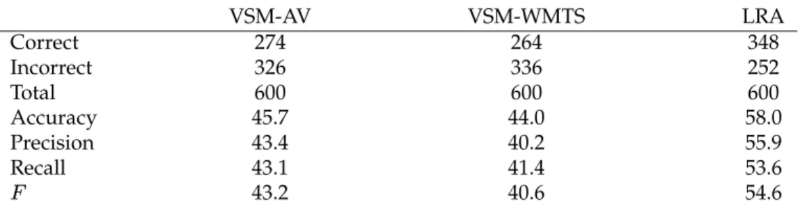
We approach the task of classifying semantic relations in noun-modifier pairs as a supervised learning problem. The 600 pairs are divided into training and testing sets and a testing pair is classified according to the label of its single nearest neighbour in the training set. LRA is used to measure distance (i.e., similarity, nearness). LRA achieves an accuracy of 39.8% on the 30-class problem and 58.0% on the 5-class problem. On the same 600 noun-modifier pairs, the VSM had accuracies of 27.8% (30-class) and 45.7% (5-class) (Turney and Littman, 2005).
We discuss the experimental results, limitations of LRA, and future work in Sec-tion 8 and we conclude in SecSec-tion 9.
2. Attributional and Relational Similarity
In this section, we explore connections between attributional and relational similarity. 2.1 Types of Similarity
Medin, Goldstone, and Gentner (1990) distinguish attributes and relations as follows:
Attributes are predicates taking one argument (e.g., is red, is large), whereas relations are predicates taking two or more arguments (e.g., collides with✁,
is larger than✁). Attributes are used to state properties of objects; relations express
relations between objects or propositions.
Gentner (1983) notes that what counts as an attribute or a relation can depend on the context. For example, large can be viewed as an attribute of✂,LARGE(✂), or a relation
between✂ and some standard✄,LARGER THAN(✂,✄).
The amount of attributional similarity between two words,☎and✆, depends on the
degree of correspondence between the properties of☎and✆. A measure of attributional
similarity is a function that maps two words,☎ and✆, to a real number,✝✞✟✠✡☎☛✆☞ ✌ ✍
. The more correspondence there is between the properties of ☎ and✆, the greater
their attributional similarity. For example, dog and wolf have a relatively high degree of attributional similarity.
The amount of relational similarity between two pairs of words, A:B and C:D, de-pends on the degree of correspondence between the relations between ☎ and ✆ and
the relations between✎ and ✏. A measure of relational similarity is a function that
maps two pairs, A:B and C:D, to a real number,✝✞✟✑✡ ☎ ✒✆☛✎ ✒✏☞ ✌ ✍
. The more cor-respondence there is between the relations of A:B and C:D, the greater their relational similarity. For example, dog:bark and cat:meow have a relatively high degree of relational
similarity.
Cognitive scientists distinguish words that are semantically associated (bee–honey) from words that are semantically similar (deer–pony), although they recognize that some words are both associated and similar (doctor–nurse) (Chiarello et al., 1990). Both of these are types of attributional similarity, since they are based on correspondence be-tween attributes (e.g., bees and honey are both found in hives; deer and ponies are both mammals).
Budanitsky and Hirst (2001) describe semantic relatedness as follows:
Recent research on the topic in computational linguistics has emphasized the perspective of semantic relatedness of two lexemes in a lexical resource, or its inverse, semantic distance. It’s important to note that semantic relatedness is a more general concept than similarity; similar entities are usually assumed to be related by virtue of their likeness (bank-trust company), but dissimilar entities may also be semantically related by lexical relationships such as meronymy (car-wheel) and antonymy (hot-cold), or just by any kind of functional relationship or frequent association (pencil-paper, penguin-Antarctica).
As these examples show, semantic relatedness is the same as attributional similarity (e.g., hot and cold are both kinds of temperature, pencil and paper are both used for writing). Here we prefer to use the term attributional similarity, because it emphasizes the contrast with relational similarity. The term semantic relatedness may lead to confu-sion when the term relational similarity is also under discusconfu-sion.
Resnik (1995) describes semantic similarity as follows:
Semantic similarity represents a special case of semantic relatedness: for example, cars and gasoline would seem to be more closely related than, say, cars and bicycles, but the latter pair are certainly more similar. Rada et al. (1989) suggest that the assessment of similarity in semantic networks can in fact be thought of as involving just taxonimic (IS-A) links, to the exclusion of other link types; that view will also be taken here, although admittedly it excludes some potentially useful information.
Thus semantic similarity is a specific type of attributional similarity. The term semantic similarity is misleading, because it refers to a type of attributional similarity, yet rela-tional similarity is not any less semantic than attriburela-tional similarity.
To avoid confusion, we will use the terms attributional similarity and relational sim-ilarity, following Medin, Goldstone, and Gentner (1990). Instead of semantic similarity (Resnik, 1995) or semantically similar (Chiarello et al., 1990), we prefer the term taxonomi-cal similarity, which we take to be a specific type of attributional similarity. We interpret synonymy as a high degree of attributional similarity. Analogy is a high degree of rela-tional similarity.
2.2 Measuring Attributional Similarity
Algorithms for measuring attributional similarity can be lexicon-based (Lesk, 1986; Bu-danitsky and Hirst, 2001; Banerjee and Pedersen, 2003), corpus-based (Lesk, 1969; Lan-dauer and Dumais, 1997; Lin, 1998a; Turney, 2001), or a hybrid of the two (Resnik, 1995; Jiang and Conrath, 1997; Turney et al., 2003). Intuitively, we might expect that lexicon-based algorithms would be better at capturing synonymy than corpus-based algorithms, since lexicons, such as WordNet, explicitly provide synonymy information that is only implicit in a corpus. However, experiments do not support this intuition.
ques-Table 2
An example of a typical TOEFL question, from the collection of 80 questions.
Stem: levied Choices: (a) imposed
(b) believed (c) requested (d) correlated Solution: (a) imposed
Table 3
Performance of attributional similarity measures on the 80 TOEFL questions. (The average non-English US college applicant’s performance is included in the bottom row, for comparison.)
Reference Description Percent Correct
Jarmasz and Szpakowicz (2003) best lexicon-based algorithm 78.75 Terra and Clarke (2003) best corpus-based algorithm 81.25 Turney et al. (2003) best hybrid algorithm 97.50 Landauer and Dumais (1997) average human score 64.50
tions taken from the Test of English as a Foreign Language (TOEFL). An example of one of the 80 TOEFL questions appears in Table 2. Table 3 shows the best performance on the TOEFL questions for each type of attributional similarity algorithm. The results support the claim that lexicon-based algorithms have no advantage over corpus-based algorithms for recognizing synonymy.
2.3 Using Attributional Similarity to Solve Analogies
We may distinguish near analogies (mason:stone::carpenter:wood) from far analogies (traffic:street::water:riverbed) (Gentner, 1983; Medin, Goldstone, and Gentner, 1990). In an analogy A:B::C:D, where there is a high degree of relational similarity between A:B and C:D, if there is also a high degree of attributional similarity between☎ and✎, and
between✆ and✏, then A:B::C:D is a near analogy; otherwise, it is a far analogy.
It seems possible that SAT analogy questions might consist largely of near analogies, in which case they can be solved using attributional similarity measures. We could score each candidate analogy by the average of the attributional similarity,✝✞✟✠, between ☎
and✎ and between✆ and✏:
✝ ✁✂✄✡☎✒✆✒✒✎ ✒✏☞☎ ✆ ✝ ✡✝✞✟ ✠ ✡☎☛✎☞✞✝✞✟ ✠ ✡ ✆☛✏☞☞ (1)
This kind of approach was used in two of the thirteen modules in Turney et al. (2003) (see Section 3.1).
To evaluate this approach, we applied several measures of attributional similarity to our collection of 374 SAT questions. The performance of the algorithms was measured by precision, recall, and✟, defined as follows:
✠
✂✄ ✞✝✞✁✡☎
✡☛✟☞✄✂✁✌ ✁✂✂✄ ✍✎☛✄✝✝✄✝ ✍✁✍✏✑✡☛✟☞✄✂✁✌✎☛✄✝✝✄✝✟✏✒✄
Table 4
Performance of attributional similarity measures on the 374 SAT questions. Precision, recall, and are reported as percentages. (The bottom two rows are not attributional similarity measures. They are included for comparison.)
Algorithm Type Precision Recall ✟
Hirst and St-Onge (1998) lexicon-based 34.9 32.1 33.4 Jiang and Conrath (1997) hybrid 29.8 27.3 28.5 Leacock and Chodorow (1998) lexicon-based 32.8 31.3 32.0
Lin (1998b) hybrid 31.2 27.3 29.1
Resnik (1995) hybrid 35.7 33.2 34.4
Turney (2001) corpus-based 35.0 35.0 35.0 Turney and Littman (2005) relational (VSM) 47.7 47.1 47.4
random random 20.0 20.0 20.0 ✂✄ ✏✑✑☎ ✡☛✟☞✄✂✁✌ ✁✂✂✄ ✍✎☛✄✝✝✄✝ ✟✏✁✞✟☛✟ ✠ ✁✝✝✞☞✑✄✡☛✟☞✄✂ ✁✂✂✄ ✍ (3) ✟ ☎ ✝ ✂ ✠ ✂✄ ✞✝✞✁✡ ✂ ✂✄ ✏✑✑ ✠ ✂✄ ✞✝✞✁✡✞✂✄ ✏✑✑ (4) Note that recall is the same as percent correct (for multiple-choice questions, with only zero or one guesses allowed per question, but not in general).
Table 4 shows the experimental results for our set of 374 analogy questions. For example, using the algorithm of Hirst and St-Onge (1998), 120 questions were answered correctly, 224 incorrectly, and 30 questions were skipped. When the algorithm assigned the same similarity to all of the choices for a given question, that question was skipped. The precision was ✆✝✄☎
✡ ✆✝✄
✞ ✝✝✆
☞and the recall was ✆✝✄☎ ✡ ✆✝✄ ✞ ✝✝✆ ✞✝ ✄ ☞.
The first five algorithms in Table 4 are implemented in Pedersen’s WordNet-Similarity package.2 The sixth algorithm (Turney, 2001) used the Waterloo MultiText System, as
described in Terra and Clarke (2003).
The difference between the lowest performance (Jiang and Conrath, 1997) and ran-dom guessing is statistically significant with 95% confidence, according to the Fisher Exact Test (Agresti, 1990). However, the difference between the highest performance (Turney, 2001) and the VSM approach (Turney and Littman, 2005) is also statistically significant with 95% confidence. We conclude that there are enough near analogies in the 374 SAT questions for attributional similarity to perform better than random guess-ing, but not enough near analogies for attributional similarity to perform as well as relational similarity.
3. Related Work
This section is a brief survey of the many problems that involve semantic relations and could potentially make use of an algorithm for measuring relational similarity.
3.1 Recognizing Word Analogies
The problem of recognizing word analogies is, given a stem word pair and a finite list of choice word pairs, select the choice that is most analogous to the stem. This problem
✞
was first attempted by a system called Argus (Reitman, 1965), using a small hand-built semantic network. Argus could only solve the limited set of analogy questions that its programmer had anticipated. Argus was based on a spreading activation model and did not explicitly attempt to measure relational similarity.
Turney et al. (2003) combined 13 independent modules to answer SAT questions. The final output of the system was based on a weighted combination of the outputs of each individual module. The best of the 13 modules was the VSM, which is described in detail in Turney and Littman (2005). The VSM was evaluated on a set of 374 SAT questions, achieving a score of 47%.
In contrast with the corpus-based approach of Turney and Littman (2005), Veale (2004) applied a lexicon-based approach to the same 374 SAT questions, attaining a score of 43%. Veale evaluated the quality of a candidate analogy A:B::C:D by looking for paths in WordNet, joining☎to✆ and✎ to✏. The quality measure was based on the
similarity between the A:B paths and the C:D paths.
Turney (2005) introduced Latent Relational Analysis (LRA), an enhanced version of the VSM approach, which reached 56% on the 374 SAT questions. Here we go beyond Turney (2005) by describing LRA in more detail, performing more extensive experi-ments, and analyzing the algorithm and related work in more depth.
3.2 Structure Mapping Theory
French (2002) cites Structure Mapping Theory (SMT) (Gentner, 1983) and its implemen-tation in the Structure Mapping Engine (SME) (Falkenhainer, Forbus, and Gentner, 1989) as the most influential work on modeling of analogy-making. The goal of computational modeling of analogy-making is to understand how people form complex, structured analogies. SME takes representations of a source domain and a target domain, and pro-duces an analogical mapping between the source and target. The domains are given structured propositional representations, using predicate logic. These descriptions in-clude attributes, relations, and higher-order relations (expressing relations between re-lations). The analogical mapping connects source domain relations to target domain relations.
For example, there is an analogy between the solar system and Rutherford’s model of the atom (Falkenhainer, Forbus, and Gentner, 1989). The solar system is the source domain and Rutherford’s model of the atom is the target domain. The basic objects in the source model are the planets and the sun. The basic objects in the target model are the electrons and the nucleus. The planets and the sun have various attributes, such as mass(sun) and mass(planet), and various relations, such as revolve(planet, sun) and attracts(sun, planet). Likewise, the nucleus and the electrons have attributes, such as charge(electron) and charge(nucleus), and relations, such as revolve(electron, nucleus) and attracts(nucleus, electron). SME maps revolve(planet, sun) to revolve(electron, nu-cleus) and attracts(sun, planet) to attracts(nucleus, electron).
Each individual connection (e.g., from revolve(planet, sun) to revolve(electron, nu-cleus)) in an analogical mapping implies that the connected relations are similar; thus, SMT requires a measure of relational similarity, in order to form maps. Early versions of SME only mapped identical relations, but later versions of SME allowed similar, non-identical relations to match (Falkenhainer, 1990). However, the focus of research in analogy-making has been on the mapping process as a whole, rather than measuring the similarity between any two particular relations, hence the similarity measures used in SME at the level of individual connections are somewhat rudimentary.
We believe that a more sophisticated measure of relational similarity, such as LRA, may enhance the performance of SME. Likewise, the focus of our work here is on the similarity between particular relations, and we ignore systematic mapping between sets
Table 5
Metaphorical sentences from Lakoff and Johnson (1980), rendered as SAT-style verbal analogies.
Metaphorical sentence SAT-style verbal analogy
He shot down all of my arguments. aircraft:shoot down::argument:refute I demolished his argument. building:demolish::argument:refute You need to budget your time. money:budget::time:schedule I’ve invested a lot of time in her. money:invest::time:allocate My mind just isn’t operating today. machine:operate::mind:think Life has cheated me. charlatan:cheat::life:disappoint Inflation is eating up our profits. animal:eat::inflation:reduce
of relations, so LRA may also be enhanced by integration with SME. 3.3 Metaphor
Metaphorical language is very common in our daily life; so common that we are usu-ally unaware of it (Lakoff and Johnson, 1980). Gentner et al. (2001) argue that novel metaphors are understood using analogy, but conventional metaphors are simply re-called from memory. A conventional metaphor is a metaphor that has become en-trenched in our language (Lakoff and Johnson, 1980). Dolan (1995) describes an algo-rithm that can recognize conventional metaphors, but is not suited to novel metaphors. This suggests that it may be fruitful to combine Dolan’s (1995) algorithm for handling conventional metaphorical language with LRA and SME for handling novel metaphors. Lakoff and Johnson (1980) give many examples of sentences in support of their claim that metaphorical language is ubiquitous. The metaphors in their sample sen-tences can be expressed using SAT-style verbal analogies of the form A:B::C:D. The first column in Table 5 is a list of sentences from Lakoff and Johnson (1980) and the second column shows how the metaphor that is implicit in each sentence may be made explicit as a verbal analogy.
3.4 Classifying Semantic Relations
The task of classifying semantic relations is to identify the relation between a pair of words. Often the pairs are restricted to noun-modifier pairs, but there are many inter-esting relations, such as antonymy, that do not occur in noun-modifier pairs. However, noun-modifier pairs are interesting due to their high frequency in English. For instance, WordNet 2.0 contains more than 26,000 noun-modifier pairs, although many common noun-modifiers are not in WordNet, especially technical terms.
Rosario and Hearst (2001) and Rosario, Hearst, and Fillmore (2002) classify noun-modifier relations in the medical domain, using MeSH (Medical Subject Headings) and UMLS (Unified Medical Language System) as lexical resources for representing each noun-modifier pair with a feature vector. They trained a neural network to distinguish 13 classes of semantic relations. Nastase and Szpakowicz (2003) explore a similar ap-proach to classifying general noun-modifier pairs (i.e., not restricted to a particular do-main, such as medicine), using WordNet and Roget’s Thesaurus as lexical resources. Vanderwende (1994) used hand-built rules, together with a lexical knowledge base, to classify noun-modifier pairs.
None of these approaches explicitly involved measuring relational similarity, but any classification of semantic relations necessarily employs some implicit notion of re-lational similarity, since members of the same class must be rere-lationally similar to some
extent. Barker and Szpakowicz (1998) tried a corpus-based approach that explicitly used a measure of relational similarity, but their measure was based on literal matching, which limited its ability to generalize. Moldovan et al. (2004) also used a measure of relational similarity, based on mapping each noun and modifier into semantic classes in WordNet. The noun-modifier pairs were taken from a corpus and the surrounding context in the corpus was used in a word sense disambiguation algorithm, to improve the mapping of the noun and modifier into WordNet. Turney and Littman (2005) used the VSM (as a component in a single nearest neighbour learning algorithm) to measure relational similarity. We take the same approach here, substituting LRA for the VSM, in Section 7.
Lauer (1995) used a corpus-based approach (using the BNC) to paraphrase noun-modifier pairs, by inserting the prepositions of, for, in, at, on, from, with, and about. For example, reptile haven was paraphrased as haven for reptiles. Lapata and Keller (2004) achieved improved results on this task, by using the database of AltaVista’s search en-gine as a corpus.
3.5 Word Sense Disambiguation
We believe that the intended sense of a polysemous word is determined by its semantic relations with the other words in the surrounding text. If we can identify the semantic relations between the given word and its context, then we can disambiguate the given word. Yarowsky’s (1993) observation that collocations are almost always monosemous is evidence for this view. Federici, Montemagni, and Pirrelli (1997) present an analogy-based approach to word sense disambiguation.
For example, consider the word plant. Out of context, plant could refer to an in-dustrial plant or a living organism. Suppose plant appears in some text near food. A typical approach to disambiguating plant would compare the attributional similarity of food and industrial plant to the attributional similarity of food and living organism (Lesk, 1986; Banerjee and Pedersen, 2003). In this case, the decision may not be clear, since in-dustrial plants often produce food and living organisms often serve as food. It would be very helpful to know the relation between food and plant in this example. In the phrase “food for the plant”, the relation between food and plant strongly suggests that the plant is a living organism, since industrial plants do not need food. In the text “food at the plant”, the relation strongly suggests that the plant is an industrial plant, since living organisms are not usually considered as locations. Thus an algorithm for classifying semantic relations (as in Section 7) should be helpful for word sense disambiguation. 3.6 Information Extraction
The problem of relation extraction is, given an input document and a specific relation , extract all pairs of entities (if any) that have the relation in the document. The prob-lem was introduced as part of the Message Understanding Conferences (MUC) in 1998. Zelenko, Aone, and Richardella (2003) present a kernel method for extracting the rela-tions person-affiliation and organization-location. For example, in the sentence “John Smith is the chief scientist of the Hardcom Corporation,” there is a person-affiliation relation between “John Smith” and “Hardcom Corporation” (Zelenko, Aone, and Richardella, 2003). This is similar to the problem of classifying semantic relations (Section 3.4), ex-cept that information extraction focuses on the relation between a specific pair of entities in a specific document, rather than a general pair of words in general text. Therefore an algorithm for classifying semantic relations should be useful for information extraction. In the VSM approach to classifying semantic relations (Turney and Littman, 2005), we would have a training set of labeled examples of the relation person-affiliation, for in-stance. Each example would be represented by a vector of pattern frequencies. Given a
specific document discussing “John Smith” and “Hardcom Corporation”, we could con-struct a vector representing the relation between these two entities, and then measure the relational similarity between this unlabeled vector and each of our labeled training vectors. It would seem that there is a problem here, because the training vectors would be relatively dense, since they would presumably be derived from a large corpus, but the new unlabeled vector for “John Smith” and “Hardcom Corporation” would be very sparse, since these entities might be mentioned only once in the given document. How-ever, this is not a new problem for the Vector Space Model; it is the standard situation when the VSM is used for information retrieval. A query to a search engine is rep-resented by a very sparse vector whereas a document is reprep-resented by a relatively dense vector. There are well-known techniques in information retrieval for coping with this disparity, such as weighting schemes for query vectors that are different from the weighting schemes for document vectors (Salton and Buckley, 1988).
3.7 Question Answering
In their paper on classifying semantic relations, Moldovan et al. (2004) suggest that an important application of their work is Question Answering. As defined in the Text RE-trieval Conference (TREC) Question Answering (QA) track, the task is to answer simple questions, such as “Where have nuclear incidents occurred?”, by retrieving a relevant document from a large corpus and then extracting a short string from the document, such as “The Three Mile Island nuclear incident caused a DOE policy crisis.” Moldovan et al. (2004) propose to map a given question to a semantic relation and then search for that relation in a corpus of semantically tagged text. They argue that the desired se-mantic relation can easily be inferred from the surface form of the question. A question of the form “Where ...?” is likely to be seeking for entities with a location relation and a question of the form “What did ... make?” is likely to be looking for entities with a product relation. In Section 7, we show how LRA can recognize relations such as location and product (see Table 19).
3.8 Automatic Thesaurus Generation
Hearst (1992) presents an algorithm for learning hyponym (type of) relations from a cor-pus and Berland and Charniak (1999) describe how to learn meronym (part of) relations from a corpus. These algorithms could be used to automatically generate a thesaurus or dictionary, but we would like to handle more relations than hyponymy and meronymy. WordNet distinguishes more than a dozen semantic relations between words (Fellbaum, 1998) and Nastase and Szpakowicz (2003) list 30 semantic relations for noun-modifier pairs. Hearst (1992) and Berland and Charniak (1999) use manually generated rules to mine text for semantic relations. Turney and Littman (2005) also use a manually gener-ated set of 64 patterns.
LRA does not use a predefined set of patterns; it learns patterns from a large corpus. Instead of manually generating new rules or patterns for each new semantic relation, it is possible to automatically learn a measure of relational similarity that can handle arbitrary semantic relations. A nearest neighbour algorithm can then use this relational similarity measure to learn to classify according to any set of classes of relations, given the appropriate labeled training data.
Girju, Badulescu, and Moldovan (2003) present an algorithm for learning meronym relations from a corpus. Like Hearst (1992) and Berland and Charniak (1999), they use manually generated rules to mine text for their desired relation. However, they supple-ment their manual rules with automatically learned constraints, to increase the precision of the rules.
3.9 Information Retrieval
Veale (2003) has developed an algorithm for recognizing certain types of word analo-gies, based on information in WordNet. He proposes to use the algorithm for ana-logical information retrieval. For example, the query “Muslim church” should return “mosque” and the query “Hindu bible” should return “the Vedas”. The algorithm was designed with a focus on analogies of the form adjective:noun::adjective:noun, such as Christian:church::Muslim:mosque.
A measure of relational similarity is applicable to this task. Given a pair of words,
☎ and ✆, the task is to return another pair of words,✂ and✄, such that there is high
relational similarity between the pair☎:✂ and the pair✄:✆. For example, given ☎ =
“Muslim” and ✆ = “church”, return ✂ = “mosque” and✄ = “Christian”. (The pair
Muslim:mosque has a high relational similarity to the pair Christian:church.)
Marx et al. (2002) developed an unsupervised algorithm for discovering analogies by clustering words from two different corpora. Each cluster of words in one corpus is coupled one-to-one with a cluster in the other corpus. For example, one experiment used a corpus of Buddhist documents and a corpus of Christian documents. A cluster of words such as Hindu, Mahayana, Zen, ...✁from the Buddhist corpus was coupled with
a cluster of words such as Catholic, Protestant, ...✁from the Christian corpus. Thus the
algorithm appears to have discovered an analogical mapping between Buddhist schools and traditions and Christian schools and traditions. This is interesting work, but it is not directly applicable to SAT analogies, because it discovers analogies between clusters of words, rather than individual words.
3.10 Identifying Semantic Roles
A semantic frame for an event such as judgement contains semantic roles such as judge, evaluee, and reason, whereas an event such as statement contains roles such as speaker, addressee, and message (Gildea and Jurafsky, 2002). The task of identifying semantic roles is to label the parts of a sentence according to their semantic roles. We believe that it may be helpful to view semantic frames and their semantic roles as sets of semantic relations; thus a measure of relational similarity should help us to identify semantic roles. Moldovan et al. (2004) argue that semantic roles are merely a special case of semantic relations (Section 3.4), since semantic roles always involve verbs or predicates, but semantic relations can involve words of any part of speech.
4. The Vector Space Model
This section examines past work on measuring attributional and relational similarity using the Vector Space Model (VSM).
4.1 Measuring Attributional Similarity with the Vector Space Model
The VSM was first developed for information retrieval (Salton and McGill, 1983; Salton and Buckley, 1988; Salton, 1989) and it is at the core of most modern search engines (Baeza-Yates and Ribeiro-Neto, 1999). In the VSM approach to information retrieval, queries and documents are represented by vectors. Elements in these vectors are based on the frequencies of words in the corresponding queries and documents. The frequen-cies are usually transformed by various formulas and weights, tailored to improve the effectiveness of the search engine (Salton, 1989). The attributional similarity between a query and a document is measured by the cosine of the angle between their correspond-ing vectors. For a given query, the search engine sorts the matchcorrespond-ing documents in order of decreasing cosine.
words (Lesk, 1969; Ruge, 1992; Pantel and Lin, 2002). Pantel and Lin (2002) clustered words according to their attributional similarity, as measured by a VSM. Their algo-rithm is able to discover the different senses of polysemous words, using unsupervised learning.
Latent Semantic Analysis enhances the VSM approach to information retrieval by using the Singular Value Decomposition (SVD) to smooth the vectors, which helps to handle noise and sparseness in the data (Deerwester et al., 1990; Dumais, 1993; Lan-dauer and Dumais, 1997). SVD improves both document-query attributional similarity measures (Deerwester et al., 1990; Dumais, 1993) and word-word attributional similar-ity measures (Landauer and Dumais, 1997). LRA also uses SVD to smooth vectors, as we discuss in Section 5.
4.2 Measuring Relational Similarity with the Vector Space Model
Let be the semantic relation (or set of relations) between a pair of words,☎ and✆,
and let ✁ be the semantic relation (or set of relations) between another pair, ✎ and ✏. We wish to measure the relational similarity between and ✁. The relations
and ✁ are not given to us; our task is to infer these hidden (latent) relations and then
compare them.
In the VSM approach to relational similarity (Turney and Littman, 2005), we create vectors,✂ and✂✁, that represent features of and ✁, and then measure the similarity
of and ✁by the cosine of the angle ✄ between✂ and✂✁: ✂ ☎ ☎✂ ✆ ☛✝✝✝☛✂ ✆✞✟ (5) ✂✁ ☎ ☎✂✁✆ ☛✝✝✝✂✁✆✞✟ (6) ✁✝✞✡✄✡ ✄ ☞☎ ✞ ✠ ✡☛ ✂ ✆ ✡ ☞ ✂✁✆ ✡ ✌ ✞ ✠ ✡☛ ✡✂ ✆ ✡ ☞ ✁ ☞ ✞ ✠ ✡☛ ✡✂✁✆ ✡ ☞ ✁ ☎ ✂ ☞ ✂✁ ✍ ✂ ☞ ✂ ☞ ✍ ✂✁ ☞ ✂✁ ☎ ✂ ☞ ✂✁ ✎ ✂ ✎ ☞ ✎ ✂✁ ✎ (7)
We create a vector,✂, to characterize the relationship between two words, ✂ and ✄, by counting the frequencies of various short phrases containing✂ and✄. Turney
and Littman (2005) use a list of 64 joining terms, such as “of”, “for”, and “to”, to form 128 phrases that contain ✂ and ✄, such as “✂ of ✄”, “✄ of ✂”, “✂ for ✄”, “✄ for ✂”, “✂ to ✄”, and “✄ to ✂”. These phrases are then used as queries for a search
engine and the number of hits (matching documents) is recorded for each query. This process yields a vector of 128 numbers. If the number of hits for a query is✏, then
the corresponding element in the vector✂is✑✁✎✡✏✞ ✆
☞. Several authors report that the
logarithmic transformation of frequencies improves cosine-based similarity measures (Salton and Buckley, 1988; Ruge, 1992; Lin, 1998b).
Turney and Littman (2005) evaluated the VSM approach by its performance on 374 SAT analogy questions, achieving a score of 47%. Since there are five choices for each question, the expected score for random guessing is 20%. To answer a multiple-choice analogy question, vectors are created for the stem pair and each choice pair, and then cosines are calculated for the angles between the stem pair and each choice pair. The best guess is the choice pair with the highest cosine. We use the same set of analogy questions to evaluate LRA in Section 6.
The VSM was also evaluated by its performance as a distance (nearness) measure in a supervised nearest neighbour classifier for noun-modifier semantic relations (Turney
and Littman, 2005). The evaluation used 600 hand-labeled noun-modifier pairs from Nastase and Szpakowicz (2003). A testing pair is classified by searching for its single nearest neighbour in the labeled training data. The best guess is the label for the training pair with the highest cosine. LRA is evaluated with the same set of noun-modifier pairs in Section 7.
Turney and Littman (2005) used the AltaVista search engine to obtain the frequency information required to build vectors for the VSM. Thus their corpus was the set of all web pages indexed by AltaVista. At the time, the English subset of this corpus consisted of about ✂ ✆✄
words. Around April 2004, AltaVista made substantial changes to their search engine, removing their advanced search operators. Their search engine no longer supports the asterisk operator, which was used by Turney and Littman (2005) for stemming and wild-card searching. AltaVista also changed their policy towards automated searching, which is now forbidden.3
Turney and Littman (2005) used AltaVista’s hit count, which is the number of docu-ments (web pages) matching a given query, but LRA uses the number of passages (strings) matching a query. In our experiments with LRA (Sections 6 and 7), we use a local copy of the Waterloo MultiText System (Clarke, Cormack, and Palmer, 1998; Terra and Clarke, 2003), running on a 16 CPU Beowulf Cluster, with a corpus of about ✂✆✄
✁
English words. The Waterloo MultiText System (WMTS) is a distributed (multiprocessor) search engine, designed primarily for passage retrieval (although document retrieval is possi-ble, as a special case of passage retrieval). The text and index require approximately one terabyte of disk space. Although AltaVista only gives a rough estimate of the number of matching documents, the Waterloo MultiText System gives exact counts of the number of matching passages.
Turney et al. (2003) combine 13 independent modules to answer SAT questions. The performance of LRA significantly surpasses this combined system, but there is no real contest between these approaches, because we can simply add LRA to the combination, as a fourteenth module. Since the VSM module had the best performance of the thirteen modules (Turney et al., 2003), the following experiments focus on comparing VSM and LRA.
5. Latent Relational Analysis
LRA takes as input a set of word pairs and produces as output a measure of the rela-tional similarity between any two of the input pairs. LRA relies on three resources, a search engine with a very large corpus of text, a broad-coverage thesaurus of synonyms, and an efficient implementation of SVD.
We first present a short description of the core algorithm. Later, in the following subsections, we will give a detailed description of the algorithm, as it is applied in the experiments in Sections 6 and 7.
✂
Given a set of word pairs as input, look in a thesaurus for synonyms for each word in each word pair. For each input pair, make alternate pairs by replacing the original words with their synonyms. The alternate pairs are intended to form near analogies with the corresponding original pairs (see Section 2.3).
✂
Filter out alternate pairs that do not form near analogies, by dropping alternate pairs that co-occur rarely in the corpus. In the preceding step, if a synonym
✄
See http://www.altavista.com/robots.txt for AltaVista’s current policy towards “robots” (software for automatically gathering web pages or issuing batches of queries). The protocol of the “robots.txt” file is explained in http://www.robotstxt.org/wc/robots.html.
replaced an ambiguous original word, but the synonym captures the wrong sense of the original word, it is likely that there is no significant relation between the words in the alternate pair, so they will rarely co-occur.
✂
For each original and alternate pair, search in the corpus for short phrases that begin with one member of the pair and end with the other. These phrases char-acterize the relation between the words in each pair.
✂
For each phrase from the previous step, create several patterns, by replacing words in the phrase with wild cards.
✂
Build a pair-pattern frequency matrix, in which each cell represents the number of times that the corresponding pair (row) appears in the corpus with the cor-responding pattern (column). The number will usually be zero, resulting in a sparse matrix.
✂
Apply the Singular Value Decomposition to the matrix. This reduces noise in the matrix and helps with sparse data.
✂
Suppose that we wish to calculate the relational similarity between any two of the original pairs. Start by looking for the two row vectors in the pair-pattern frequency matrix that correspond to the two original pairs. Calculate the co-sine of the angle between these two row vectors. Then merge the coco-sine of the two original pairs with the cosines of their corresponding alternate pairs, as fol-lows. If an analogy formed with alternate pairs has a higher cosine than the original pairs, we assume that we have found a better way to express the anal-ogy, but we have not significantly changed its meaning. If the cosine is lower, we assume that we may have changed the meaning, by inappropriately replac-ing words with synonyms. Filter out inappropriate alternates by droppreplac-ing all analogies formed of alternates, such that the cosines are less than the cosine for the original pairs. The relational similarity between the two original pairs is then calculated as the average of all of the remaining cosines.
The motivation for the alternate pairs is to handle cases where the original pairs co-occur rarely in the corpus. The hope is that we can find near analogies for the original pairs, such that the near analogies co-occur more frequently in the corpus. The danger is that the alternates may have different relations from the originals. The filtering steps above aim to reduce this risk.
5.1 Input and Output
In our experiments, the input set contains from 600 to 2,244 word pairs. The output similarity measure is based on cosines, so the degree of similarity can range from ✆
(dissimilar; ✄ ☎ ✆✁✄✂ ) to ✞ ✆ (similar; ✄ ☎ ✄✂
). Before applying SVD, the vectors are completely nonnegative, which implies that the cosine can only range from✄
to✞ ✆
, but SVD introduces negative values, so it is possible for the cosine to be negative, although we have never observed this in our experiments.
5.2 Search Engine and Corpus
In the following experiments, we use a local copy of the Waterloo MultiText System (Clarke, Cormack, and Palmer, 1998; Terra and Clarke, 2003).4 The corpus consists of
about ✂✆✄ ✁
English words, gathered by a web crawler, mainly from US academic
✄
web sites. The web pages cover a very wide range of topics, styles, genres, quality, and writing skill. The WMTS is well suited to LRA, because the WMTS scales well to large corpora (one terabyte, in our case), it gives exact frequency counts (unlike most web search engines), it is designed for passage retrieval (rather than document retrieval), and it has a powerful query syntax.
5.3 Thesaurus
As a source of synonyms, we use Lin’s (1998a) automatically generated thesaurus. This thesaurus is available through an online interactive demonstration or it can be down-loaded.5 We used the online demonstration, since the downloadable version seems to
contain fewer words. For each word in the input set of word pairs, we automatically query the online demonstration and fetch the resulting list of synonyms. As a courtesy to other users of Lin’s online system, we insert a 20 second delay between each query.
Lin’s thesaurus was generated by parsing a corpus of about ✂✆✄
English words, consisting of text from the Wall Street Journal, San Jose Mercury, and AP Newswire (Lin, 1998a). The parser was used to extract pairs of words and their grammatical relations. Words were then clustered into synonym sets, based on the similarity of their grammat-ical relations. Two words were judged to be highly similar when they tended to have the same kinds of grammatical relations with the same sets of words. Given a word and its part of speech, Lin’s thesaurus provides a list of words, sorted in order of decreasing attributional similarity. This sorting is convenient for LRA, since it makes it possible to focus on words with higher attributional similarity and ignore the rest. WordNet, in contrast, given a word and its part of speech, provides a list of words grouped by the possible senses of the given word, with groups sorted by the frequencies of the senses. WordNet’s sorting does not directly correspond to sorting by degree of attributional similarity, although various algorithms have been proposed for deriving attributional similarity from WordNet (Resnik, 1995; Jiang and Conrath, 1997; Budanitsky and Hirst, 2001; Banerjee and Pedersen, 2003).
5.4 Singular Value Decomposition
We use Rohde’s SVDLIBC implementation of the Singular Value Decomposition, which is based on SVDPACKC (Berry, 1992).6 In LRA, SVD is used to reduce noise and
com-pensate for sparseness. 5.5 The Algorithm
We will go through each step of LRA, using an example to illustrate the steps. Assume that the input to LRA is the 374 multiple-choice SAT word analogy questions of Tur-ney and Littman (2005). Since there are six word pairs per question (the stem and five choices), the input consists of 2,244 word pairs. Let’s suppose that we wish to calculate the relational similarity between the pair quart:volume and the pair mile:distance, taken from the SAT question in Table 6. The LRA algorithm consists of the following twelve steps:
1. Find alternates: For each word pair☎:✆ in the input set, look in Lin’s (1998a)
thesaurus for the top✁✂✄ ☎ ✆
✄ words (in the following experiments,✁✂✄ ☎ ✆
✄
is 10) that are most similar to ☎. For each ☎✝that is similar to ☎, make a new
word pair☎✝:✆. Likewise, look for the top✁✂✄ ☎ ✆
✄words that are most similar ✞
The online demonstration is at http://www.cs.ualberta.ca/✟lindek/demos/depsim.htm and the
downloadable version is at http://armena.cs.ualberta.ca/lindek/downloads/sims.lsp.gz.✟
SVDLIBC is available at http://tedlab.mit.edu/✟dr/SVDLIBC/ and SVDPACKC is available at
Table 6
This SAT question, from Claman (2000), is used to illustrate the steps in the LRA algorithm.
Stem: quart:volume Choices: (a) day:night
(b) mile:distance (c) decade:century (d) friction:heat (e) part:whole Solution: (b) mile:distance
to✆, and for each✆✝, make a new word pair☎:✆✝.☎:✆ is called the original pair
and each ☎✝:✆ or☎:✆✝ is an alternate pair. The intent is that alternates should
have almost the same semantic relations as the original. For each input pair, there will now be✝✂
✁✂✄ ☎ ✆
✄alternate pairs. When looking for similar words
in Lin’s (1998a) thesaurus, avoid words that seem unusual (e.g., hyphenated words, words with three characters or less, words with non-alphabetical char-acters, multi-word phrases, and capitalized words). The first column in Table 7 shows the alternate pairs that are generated for the original pair quart:volume. 2. Filter alternates: For each original pair☎:✆, filter the
✝ ✂ ✁✂✄ ☎
✆
✄ alternates
as follows. For each alternate pair, send a query to the WMTS, to find the frequency of phrases that begin with one member of the pair and end with the other. The phrases cannot have more than ✄ ✏ ✁✂✂ ☎✄ words (we use ✄ ✏ ✁✂✂ ☎✄ ☎ ). Sort the alternate pairs by the frequency of their phrases.
Select the top✁✂✄ ☎ ✆✆✝
✄✂most frequent alternates and discard the remainder
(we use ✁✂✄ ☎ ✆✆✝
✄✂ ☎ ✝, so 17 alternates are dropped). This step tends to
eliminate alternates that have no clear semantic relation. The third column in Table 7 shows the frequency with which each pair co-occurs in a window of
✄ ✏ ✁✂✂ ☎✄words. The last column in Table 7 shows the pairs that are selected.
3. Find phrases: For each pair (originals and alternates), make a list of phrases in the corpus that contain the pair. Query the WMTS for all phrases that begin with one member of the pair and end with the other (in either order). We ig-nore suffixes when searching for phrases that match a given pair. The phrases cannot have more than✄ ✏ ✁✂✂ ☎✄words and there must be at least one word
between the two members of the word pair. These phrases give us information about the semantic relations between the words in each pair. A phrase with no words between the two members of the word pair would give us very little information about the semantic relations (other than that the words occur to-gether with a certain frequency in a certain order). Table 8 gives some examples of phrases in the corpus that match the pair quart:volume.
4. Find patterns: For each phrase found in the previous step, build patterns from the intervening words. A pattern is constructed by replacing any or all or none of the intervening words with wild cards (one wild card can only replace one word). If a phrase is✁words long, there are✁
✝
intervening words between the members of the given word pair (e.g., between quart and volume). Thus a phrase with✁words generates
✝✞ ✞✟✁✠
patterns. (We use✄ ✏ ✁✂✂ ☎✄ ☎ , so a
Table 7
Alternate forms of the original pair quart:volume. The first column shows the original pair and the alternate pairs. The second column shows Lin’s similarity score for the alternate word compared to the original word. For example, the similarity between quart and pint is 0.210. The third column shows the frequency of the pair in the WMTS corpus. The fourth column shows the pairs that pass the filtering step (i.e., step 2).
Word pair Similarity Frequency Filtering step quart:volume NA 632 accept (original pair)
pint:volume 0.210 372
gallon:volume 0.159 1500 accept (top alternate) liter:volume 0.122 3323 accept (top alternate)
squirt:volume 0.084 54
pail:volume 0.084 28
vial:volume 0.084 373
pumping:volume 0.073 1386 accept (top alternate)
ounce:volume 0.071 430 spoonful:volume 0.070 42 tablespoon:volume 0.069 96 quart:turnover 0.229 0 quart:output 0.225 34 quart:export 0.206 7 quart:value 0.203 266 quart:import 0.186 16 quart:revenue 0.185 0 quart:sale 0.169 119 quart:investment 0.161 11 quart:earnings 0.156 0 quart:profit 0.156 24 Table 8
Some examples of phrases that contain quart:volume. Suffixes are ignored when searching for matching phrases in the WMTS corpus. At least one word must occur between quart and volume. At most ✁✂✄☎✆✁✝✞words can appear in a phrase.
“quarts liquid volume” “volume in quarts” “quarts of volume” “volume capacity quarts”
“quarts in volume” “volume being about two quarts” “quart total volume” “volume of milk in quarts”
Table 9
Frequencies of various patterns for quart:volume. The asterisk “*” represents the wildcard. Suffixes are ignored, so “quart” matches “quarts”. For example, “quarts in volume” is one of the four phrases that match “quart volume” when is “in”.
✁ = “in” ✁ = “* of” ✁ = “of *” ✁ = “* *” freq(“quart✁ volume”) 4 1 5 19 freq(“volume✁ quart”) 10 0 2 16
of pairs (originals and alternates) with phrases that match the pattern (a wild card must match exactly one word). Keep the top✁✂✄ ✁
✝✝
✄✂✁☎most frequent
patterns and discard the rest (we use ✁✂✄ ✁ ✝✝ ✄✂✁☎ ☎ ✆ ☛ ✄✄✄ ). Typically there will be millions of patterns, so it is not feasible to keep them all.
5. Map pairs to rows: In preparation for building the matrix✂, create a mapping
of word pairs to row numbers. For each pair ☎:✆, create a row for☎:✆ and
another row for ✆:☎. This will make the matrix more symmetrical, reflecting
our knowledge that the relational similarity between ☎:✆ and ✎:✏ should be
the same as the relational similarity between✆:☎ and✏:✎. This duplication of
rows is examined in Section 6.6.
6. Map patterns to columns: Create a mapping of the top✁✂✄ ✁ ✝✝
✄✂✁☎patterns
to column numbers. For each pattern✁
, create a column for “✄☎✂✆ ✁
✄☎✂✆✁”
and another column for “✄☎✂✆✁ ✁
✄☎✂✆ ”. Thus there will be ✝✂
✁✂✄ ✁ ✝✝
✄✂✁☎
columns in✂. This duplication of columns is examined in Section 6.6.
7. Generate a sparse matrix: Generate a matrix✂ in sparse matrix format,
suit-able for input to SVDLIBC. The value for the cell in row ✆
and column ✝ is
the frequency of the ✝-th pattern (see step 6) in phrases that contain the ✆
-th word pair (see step 5). Table 9 gives some examples of pattern frequencies for quart:volume.
8. Calculate entropy: Apply log and entropy transformations to the sparse matrix (Landauer and Dumais, 1997). These transformations have been found to be very helpful for information retrieval (Harman, 1986; Dumais, 1990). Let✏
✡ ✆
✞
be the cell in row ✆
and column✝ of the matrix✂ from step 7. Let ✄ be the
number of rows in✂ and let✁be the number of columns. We wish to weight
the cell✏ ✡
✆ ✞
by the entropy of the✝-th column. To calculate the entropy of the
column, we need to convert the column into a vector of probabilities. Let✁ ✡ ✆ ✞ be the probability of✏ ✡ ✆ ✞
, calculated by normalizing the column vector so that the sum of the elements is one,✁
✡ ✆ ✞ ☎ ✏ ✡ ✆ ✞ ☎ ✠✟ ✠☛ ✏ ✠ ✆ ✞
. The entropy of the✝-th
column is then ✡ ✞ ☎ ✠✟ ✠☛ ✁ ✠ ✆ ✞ ✑✁✎✡✁ ✠ ✆ ✞
☞. Entropy is at its maximum when ✁ ✡ ✆ ✞ is a uniform distribution,✁ ✡ ✆ ✞ ☎ ✆☎ ✄, in which case✡ ✞ ☎ ✑✁✎✡✄☞. Entropy
is at its minimum when✁ ✡
✆ ✞
is 1 for some value of✆
and 0 for all other values of ✆
, in which case ✡ ✞
☎ ✄
. We want to give more weight to columns (pat-terns) with frequencies that vary substantially from one row (word pair) to the next, and less weight to columns that are uniform. Therefore we weight the cell✏ ✡ ✆ ✞ by✄ ✞ ☎ ✆ ✡ ✞ ☎
✑✁✎✡✄☞, which varies from 0 when✁ ✡
✆ ✞
is uniform to 1 when entropy is minimal. We also apply the log transformation to frequen-cies, ✑✁✎✡✏ ✡ ✆ ✞ ✞ ✆
☞. (Entropy is calculated with the original frequency values,
before the log transformation is applied.) For all✆
value✏ ✡
✆ ✞
in✂ by the new value✄ ✞ ✑✁✎✡✏ ✡ ✆ ✞ ✞ ✆
☞. This is an instance of the
TF-IDF (Term Frequency-Inverse Document Frequency) family of transformations, which is familiar in information retrieval (Salton and Buckley, 1988; Baeza-Yates and Ribeiro-Neto, 1999):✑✁✎✡✏ ✡ ✆ ✞ ✞ ✆
☞is the TF term and✄ ✞
is the IDF term. 9. Apply SVD: After the log and entropy transformations have been applied to
the matrix ✂, run SVDLIBC. SVD decomposes a matrix✂ into a product of
three matrices ✁✂✄, where and ✂ are in column orthonormal form (i.e.,
the columns are orthogonal and have unit length: ✄ ☎ ✂✄✂ ☎ ☎) and ✁ is a diagonal matrix of singular values (hence SVD) (Golub and Loan, 1996).
If ✂ is of rank✂, then ✁ is also of rank ✂. Let ✁ ✠
, where ✆ ✝ ✂, be the
di-agonal matrix formed from the top ✆ singular values, and let ✠
and ✂ ✠
be the matrices produced by selecting the corresponding columns from and✂.
The matrix ✠ ✁
✠ ✂✄
✠ is the matrix of rank
✆ that best approximates the
orig-inal matrix ✂, in the sense that it minimizes the approximation errors. That
is, ✞ ✂ ☎ ✠ ✁ ✠ ✂✄ ✠ minimizes ✟ ✟ ✟ ✞ ✂ ✂ ✟ ✟ ✟
✠ over all matrices ✞
✂ of rank✆, where ✎
✝✝✝ ✎
✠ denotes the Frobenius norm (Golub and Loan, 1996). We may think of
this matrix ✠ ✁
✠ ✂✄
✠ as a “smoothed” or “compressed” version of the
origi-nal matrix. In the subsequent steps, we will be calculating cosines for row vectors. For this purpose, we can simplify calculations by dropping ✂. The
cosine of two vectors is their dot product, after they have been normalized to unit length. The matrix✂✂
✄ contains the dot products of all of the row
vec-tors. We can find the dot product of the ✆
-th and✝-th row vectors by
look-ing at the cell in row ✆
, column✝ of the matrix ✂✂
✄. Since
✂✄✂ ☎ ☎, we
have✂✂ ✄
☎ ✁✂✄✡ ✁✂✄☞✄ ☎ ✁✂✄✂✁✄ ✄ ☎ ✁✡ ✁☞✄, which means
that we can calculate cosines with the smaller matrix ✁, instead of using ✂ ☎ ✁✂✄ (Deerwester et al., 1990). 10. Projection: Calculate ✠ ✁ ✠ (we use✆ ☎ ✝ ✄✄
). This matrix has the same number of rows as ✂, but only ✆ columns (instead of
✝ ✂ ✁✂✄ ✁
✝✝
✄✂✁☎ columns; in
our experiments, that is 300 columns instead of 8,000). We can compare two word pairs by calculating the cosine of the corresponding row vectors in ✠
✁ ✠
. The row vector for each word pair has been projected from the original 8,000 dimensional space into a new 300 dimensional space. The value ✆ ☎ ✝
✄✄
is recommended by Landauer and Dumais (1997) for measuring the attributional similarity between words. We investigate other values in Section 6.4.
11. Evaluate alternates: Let ☎:✆ and ✎:✏ be any two word pairs in the input
set. From step 2, we have ✡✁✂✄ ☎ ✆✆✝
✄✂ ✞ ✆
☞versions of☎:✆, the original and ✁✂✄ ☎
✆✆✝
✄✂ alternates. Likewise, we have ✡✁✂✄ ☎ ✆✆✝ ✄✂ ✞ ✆ ☞ versions of ✎:✏. Therefore we have ✡✁✂✄ ☎ ✆✆✝ ✄✂✞ ✆ ☞ ✁
ways to compare a version of ☎:✆ with
a version of ✎:✏. Look for the row vectors in ✠
✁ ✠
that correspond to the versions of ☎:✆ and the versions of✎:✏ and calculate the ✡✁✂✄ ☎
✆✆✝ ✄✂ ✞
✆ ☞
✁
cosines (in our experiments, there are 16 cosines). For example, suppose ☎:✆
is quart:volume and ✎:✏ is mile:distance. Table 10 gives the cosines for the
sixteen combinations.
12. Calculate relational similarity: The relational similarity between☎:✆ and✎:✏
is the average of the cosines, among the✡✁✂✄ ☎ ✆✆✝
✄✂✞ ✆
☞ ✁
cosines from step 11, that are greater than or equal to the cosine of the original pairs,☎:✆ and✎:✏.
The requirement that the cosine must be greater than or equal to the original cosine is a way of filtering out poor analogies, which may be introduced in step
Table 10
The sixteen combinations and their cosines. :✁::✂:✄expresses the analogy “ is to✁as✂is to ✄”. The third column indicates those combinations for which the cosine is greater than or equal
to the cosine of the original analogy, quart:volume::mile:distance.
Word pairs Cosine Cosine☎original pairs
quart:volume::mile:distance 0.525 yes (original pairs) quart:volume::feet:distance 0.464 quart:volume::mile:length 0.634 yes quart:volume::length:distance 0.499 liter:volume::mile:distance 0.736 yes liter:volume::feet:distance 0.687 yes liter:volume::mile:length 0.745 yes liter:volume::length:distance 0.576 yes gallon:volume::mile:distance 0.763 yes gallon:volume::feet:distance 0.710 yes
gallon:volume::mile:length 0.781 yes (highest cosine) gallon:volume::length:distance 0.615 yes
pumping:volume::mile:distance 0.412 pumping:volume::feet:distance 0.439 pumping:volume::mile:length 0.446 pumping:volume::length:distance 0.491
1 and may have slipped through the filtering in step 2. Averaging the cosines, as opposed to taking their maximum, is intended to provide some resistance to noise. For quart:volume and mile:distance, the third column in Table 10 shows which alternates are used to calculate the average. For these two pairs, the average of the selected cosines is 0.677. In Table 7, we see that pumping:volume has slipped through the filtering in step 2, although it is not a good alternate for quart:volume. However, Table 10 shows that all four analogies that involve pumping:volume are dropped here, in step 12.
Steps 11 and 12 can be repeated for each two input pairs that are to be compared. This completes the description of LRA.
Table 11 gives the cosines for the sample SAT question. The choice pair with the highest average cosine (the choice with the largest value in column #1), choice (b), is the solution for this question; LRA answers the question correctly. For comparison, column #2 gives the cosines for the original pairs and column #3 gives the highest cosine. For this particular SAT question, there is one choice that has the highest cosine for all three columns, choice (b), although this is not true in general. Note that the gap between the first choice (b) and the second choice (d) is largest for the average cosines (column #1). This suggests that the average of the cosines (column #1) is better at discriminating the correct choice than either the original cosine (column #2) or the highest cosine (column #3).
6. Experiments with Word Analogy Questions
This section presents various experiments with 374 multiple-choice SAT word analogy questions.
Table 11
Cosines for the sample SAT question given in Table 6. Column #1 gives the averages of the cosines that are greater than or equal to the original cosines (e.g., the average of the cosines that are marked “yes” in Table 10 is 0.677; see choice (b) in column #1). Column #2 gives the cosine for the original pairs (e.g., the cosine for the first pair in Table 10 is 0.525; see choice (b) in column #2). Column #3 gives the maximum cosine for the sixteen possible analogies (e.g., the maximum cosine in Table 10 is 0.781; see choice (b) in column #3).
Average Original Highest cosines cosines cosines
Stem: quart:volume #1 #2 #3
Choices: (a) day:night 0.374 0.327 0.443
(b) mile:distance 0.677 0.525 0.781 (c) decade:century 0.389 0.327 0.470 (d) friction:heat 0.428 0.336 0.552 (e) part:whole 0.370 0.330 0.408 Solution: (b) mile:distance 0.677 0.525 0.781 Gap: (b)-(d) 0.249 0.189 0.229 Table 12
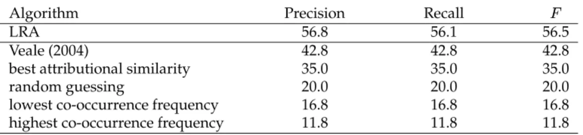
Performance of LRA on the 374 SAT questions. Precision, recall, and are reported as percentages. (The bottom five rows are included for comparison.)
Algorithm Precision Recall ✟
LRA 56.8 56.1 56.5
Veale (2004) 42.8 42.8 42.8
best attributional similarity 35.0 35.0 35.0
random guessing 20.0 20.0 20.0
lowest co-occurrence frequency 16.8 16.8 16.8 highest co-occurrence frequency 11.8 11.8 11.8
6.1 Baseline LRA System
Table 12 shows the performance of the baseline LRA system on the 374 SAT questions, using the parameter settings and configuration described in Section 5. LRA correctly answered 210 of the 374 questions. 160 questions were answered incorrectly and 4 ques-tions were skipped, because the stem pair and its alternates were represented by zero vectors. The performance of LRA is significantly better than the lexicon-based approach of Veale (2004) (see Section 3.1) and the best performance using attributional similarity (see Section 2.3), with 95% confidence, according to the Fisher Exact Test (Agresti, 1990). As another point of reference, consider the simple strategy of always guessing the choice with the highest co-occurrence frequency. The idea here is that the words in the solution pair may occur together frequently, because there is presumably a clear and meaningful relation between the solution words, whereas the distractors may only occur together rarely, because they have no meaningful relation. This strategy is signif-cantly worse than random guessing. The opposite strategy, always guessing the choice pair with the lowest co-occurrence frequency, is also worse than random guessing (but not significantly). It appears that the designers of the SAT questions deliberately chose distractors that would thwart these two strategies.