Any correspondence concerning this service should be sent
to the repository administrator:
[email protected]
This is an author’s version published in:
http://oatao.univ-toulouse.fr/22542
Official URL
DOI :
https://aaai.org/ocs/index.php/AAAI/AAAI18/paper/view/17272
Open Archive Toulouse Archive Ouverte
OATAO is an open access repository that collects the work of Toulouse
researchers and makes it freely available over the web where possible
To cite this version:
Fargier, Hélène and Gimenez,
Pierre-François and Mengin, Jérôme Learning Lexicographic Preference
Trees From Positive Examples. (2018) In: 32th AAAI Conference
on Artificial Intelligence (AAAI 2018), 2 February 2018 - 7
February 2018 (New Orleans, United States).
Abstract
This paper considers the task of learning the preferences of users on a combinatorial set of alternatives, as it can be the case for example with online configurators. In many settings, what is available to the learner is a set of positive examples of alternatives that have been selected during past interactions. We propose to learn a model of the users’ preferences that ranks previously chosen alternatives as high as possible. In this paper, we study the particular task of learning conditional lexicographic preferences. We present an algorithm to learn several classes of lexicographic preference trees, prove con-vergence properties of the algorithm, and experiment on both synthetic data and on a real-world bench in the domain of recommendation in interactive configuration.
1
Introduction
Modern, interactive decision support systems like recom-mender systems or configurators often handle a very large set of possible decisions/alternatives. The task of finding the alternatives that best suit their preferences can be challeng-ing for users, but the system can guide them towards their optimal decision if it has some knowledge of their pref-erences. In many settings, the users’ preferences are not known in advance. This is especially the case of systems that enable anonymous users to browse the catalogues: such systems must be able to acquire users’ preferences.
That is why preference learning has emerged in the last decade as an important field; many interesting results are re-ported in e.g. the book edited by (F¨urnkranz and H¨ullermeier 2011), or the proceedings of recent Preference Learning or DA2PL (Decision Aid to Preference Learning) workshops. A general problem is: given a set of observed preferences, induce a model of preferences that best explains these ob-servations, within a certain class of models. As input, it is often assumed that the observed preferences are given as a set of pairwise comparisons or partial rankings of alterna-tives (Joachims 2002); or can be elicitated online by asking the user to choose between two alternatives (Viappiani, Falt-ings, and Pu 2006; Koriche and Zanuttini 2009).
But in some circumstances, such input is not available. This is especially the case of some anonymous on-line con-figurators, where little information is stored about
interac-tions. However, e-commerce companies in general keep a history of past sales. Sold items have been chosen by users, so they must be ranked high in their preferences, but not nec-essarily in the very top; indeed a user may be led to eventu-ally choose an item which is not the optimal one in her pref-erence order: for instance because of the difficulty to grasp all possible options, a phenomenon called “mass confusion” (Huffman and Kahn 1998), because of the influence of an advertisement, or because her preferred item is unavailable. Yet, this list of highly ranked items does provide information about the users’ preferences.
Our aim in this paper is to study how the users’ prefer-ences can be learnt from this sales history. Note that this is different from a classification problem where one would want to separate alternatives between, say, acceptable ones and not acceptable ones. In our problem, we want to rank the alternatives. If, for instance, the colour red appears more of-ten in the sales history than the colour yellow, then we want to induce a model that ranks alternatives with the colour red higher than alternatives with the colour yellow – maybe in association with some other criteria.
Research on the representation and learning of prefer-ences has brought forward several types of models. Numer-ical models, like linear ranking functions or additive util-ities (Joachims 2002; Freund et al. 2003; Schiex, Fargier, and Verfaillie 1995; Gonzales and Perny 2004; Braziunas 2005), are rich families of models, especially if one allows high-dimensional feature spaces. Research in Artificial In-telligence has also brought forward ordinal models, like CP-nets (Boutilier et al. 2004) and several extensions or vari-ants. Lexicographic preferences are another family of ordi-nal models. This kind of preference is based on the impor-tance of the attributes: when comparing two outcomes, their values for the most important attribute are compared; if the two outcomes have different values for that attribute, then the one with the preferred value is deemed preferable to the other; otherwise one looks at the next most important at-tribute, and so on. This model can be extended by allowing the preferences on the values of an issue to depend on the values of more important ones. The relative importance of issues is no longer a linear order, but a “lexicographic pref-erence” tree (Fraser 1993; 1994; Brewka and others 2006; Wallace and Wilson 2009; Booth et al. 2010).
Lexicographic preference trees are the model that we
Learning
Lexicographic Preference Trees from Positive Examples
H´el`ene
Fargier, Pierre-Franc¸ois Gimenez, J´erˆome Mengin
IRIT, CNRS, University of Toulouse, 31000 Toulouse, France {fargier, pgimenez, mengin}@irit.fr
choose in this paper for two main reasons. First, this is an ordinal model, which is sufficient to represent a ranking of alternatives. Furthermore, the restricted expressivity of the lexicographic preference trees makes them easier to learn while being generally an accurate representation of human behaviours (Gigerenzer and Goldstein 1996). Finally, one can quickly (in polytime) perform some interesting requests for recommendation, such as finding an optimal object or an optimal value for some attribute.
Learning lexicographic preference models have been studied by e.g. (Schmitt and Martignon 2006; Dombi, Im-reh, and Vincze 2007; Yaman et al. 2008), while (Booth et al. 2010; Br¨auning and H¨ullermeyer 2012; Br¨auning et al. 2017; Liu and Truszczynski 2015) studied learning of lexi-cographic preference trees. But all these works assume sets of pairwise comparisons as inputs, while we seek to learn from sales history. Preference learning is also different from learning a (lexicographic) rank-based classifier, as proposed by e.g. (Flach and Matsubara 2007): the latter task takes as input a set of positive and negative instances of a concept.
The paper is structured as follows. The next Section sum-marizes the lexicographic preference tree models and intro-duces the LP-tree classes we aim to learn. Section 3 details the probabilistic model on which our approach is based. The algorithmics is developed in Section 4. Section 5 describes experiments on synthetic data and Section 6 on a real-world dataset in the domain of recommendation in interactive con-figuration.
2
Lexicographic preference trees
Notations
We consider a combinatorial domain over a setX of n dis-crete attributes, each attributeX having a finite domain X. An outcome is an instantiation of X . We use upper-case, bold letters to represent tuples of attributes; if U is such a tuple, then the set of assignments of U is denoted by U, and the corresponding lower-case letter will generally de-note such an assignment: u∈ U. A (complete) outcome is therefore a tuple o∈Q
X∈XX; we denote by X the set of
all of them. o[U] denotes the projection of o onto U: it is a partial outcome, i.e. an instantiation of U; we say that o extends o[U].
If U and V are disjoint tuples of attributes, UV will de-note their concatenation – with similar notations for assign-ments: if u ∈ U and v ∈ V then uv ∈ UV. If U and V are not disjoint, we say that u and v are compatible if u[U ∩ V] = v[U ∩ V].
A preference is modelled as a transitive binary relation over the domain of interest,X in our case. We consider in this paper that indifference is not allowed; the relation is said to be strict and we denote it ≻: o ≻ o′ indicates that o is
(strictly) preferred to o′. We denote by rank(≻, o) the rank of outcome o in the relation≻: the “best” outcome has rank 1, the worst has rank|X |.
Lexicographic preference trees
In the formal model proposed by (Booth et al. 2010), a lexi-cographic preference tree, or LP-tree for short, is composed
of two parts: a rooted tree indicating the relative importance of the attributes, and tables indicating how to compare out-comes that agree on some attributes. Each node of the im-portance tree is labelled with an attribute X ∈ X , and is either a leaf of the tree, or has one single, unlabelled outgo-ing edge, or has|X| outgoing edges, each one being labelled with one of these values. No attribute can appear twice in a branch. For a given nodeN , Anc(N ) denotes the set of at-tributes that label nodes above N . The values of attributes that are at a node aboveN with a labelled outgoing edge in-fluence the preference atN . We denote by Inst(N ) the set of nodes aboveN with a labelled outgoing edge and inst(N ) the tuple of values of the labels between the root andN . Example 1. An example of a LP-tree is depicted in Fig-ure 1a. Let N be the leftmost leaf labelled C, we have Anc(N ) = {A, B} and inst(N ) = a.
Moreover, one conditional preference table CPT(N ) is associated to each nodeN of the tree: if X is the attribute that labels N , then the table contains (consistent) rules of the form v : >, where v is a (possibly partial) instantiation of the attributes in Anc(N ) r Inst(N ), and > is a strict to-tal order > over X. Every LP-tree L induces a (possibly partial) strict order overX , denoted ≻L, as follows: for any
nodeN labelled by X, consider a pair of complete outcomes oand o′such that o[Inst(N )] = o′[Inst(N )] = inst(N ) and
o[V] = o′[V] = v for some rule v : > in CPT(N ) with
v ∈ V; N is said to decide the pair (o, o′), and o ≻ L o′if
and only if o[X] > o′[X].
A branch of a tree is complete iff all attributes appear in it; if all the branches of a tree are complete, then the tree itself is said to be complete. The preference relation induced by a LP-tree is total if and only if the tree is complete (Br¨auning and H¨ullermeyer 2012). In this case, every outcome has a well-defined rank in the preference relation (and there is only one optimal outcome, ranked 1). (Lang, Mengin, and Xia 2012) have shown that it can be computed in polytime and that, for a given rank, finding an outcome with that rank can also be done in polytime. In the following, we will deal with complete trees and ranking only.
Linear LP-trees and
k-LP-trees
In this paper, in addition to general LP-trees, we will be in-terested in a syntactic restriction called linear LP-tree and a extension calledk-LP-tree.
A linear LP-tree is a LP-tree with a single branch and un-conditional preference rules only, like the tree in Figure 1b. It is a strong expressive restriction: linear LP-trees represent the usual, unconditional lexicographic preference relations, and corresponds to LP-trees with unconditional local pref-erences and unconditional importance relation as defined by (Booth et al. 2010).
(Br¨auning and H¨ullermeyer 2012; Br¨auning et al. 2017) extend the expressiveness of LP-trees by allowing to label a node with a set of attributes, considered as a single high-dimensional attribute: the rules in the conditional preference table of the node define orders on the Cartesian product of the domains of its attributes. Note that any (strict) preference relation can in principle be represented by such a LP-tree –
A a > ¯a B a b > ¯b C ¯ a ¯ c > c C b : c > ¯c ¯b : ¯c > c ¯b > b B abc ≻ ab¯c ≻ a¯b¯c ≻ a¯bc ≻ ¯a¯b¯c ≻ ¯ab¯c ≻ ¯a¯bc ≻ ¯abc
(a) A LP-tree.
A a > ¯a B b > ¯b C ¯c > c
ab¯c ≻ abc ≻ a¯b¯c ≻ a¯bc ≻ ¯ab¯c ≻ ¯abc ≻ ¯a¯b¯c ≻ ¯a¯bc
(b) A linear LP-tree
A a > ¯a
BC bc > ¯b¯c > ¯bc > b¯c abc ≻ a¯b¯c ≻ a¯bc ≻ ab¯c ≻ ¯abc ≻ ¯a¯b¯c ≻ ¯a¯bc ≻ ¯ab¯c
(c) A 2-LP-tree Figure 1: Different LP-trees and the preference relations they induce.
possibly by labelling the root with a set that contains all at-tributes and an order over the full domainX . Generally, we restrict this expressivity by fixing the maximum number of attributes labelling a node. We denote k-LP-tree the trees whose nodes are labelled by at mostk attributes. Figure 1c shows a 2-LP-tree whose preference relation cannot be ex-pressed with a regular LP-tree.
3
Learning a preference relation from sales
histories
The probabilistic model
As exposed in the introduction, the input of the learning pro-cess is a sales history, i.e. a multisetH ⊆ X . Its elements are positive examples, outcomes corresponding to products that may have been, for instance, configured by users of some configurator and bought. Each user has a preference rela-tion ˘≻ among products, and is free to configure the prod-ucts according to her preference. However, for some reasons like the influence of advertisements, she may end up with a product which is not her most preferred one.Yet, the higher an outcome is ranked in the user’s preference, the greater the probability that she ends up with it.
Formally, our idea is to consider that there is a ground, hidden preference relation ˘≻, and an associated probability distributionp≻˘ overX which is decreasing and monotonic
w.r.t. ˘≻, i.e. if o ˘≻ o′ thenp ˘
≻(o) ≥ p≻˘(o′). We consider
thatH is a set of outcomes that have been drawn according to the distributionp≻˘. In this paper, we study the problem of
learning a LP-treeL which explains H.
In practice, we can split the learning setH into several clusters and thus reduce the variability of the preferences inside each cluster. Even though each cluster includes the preference of multiple users, they have similar preferences, which can be represented with a unique ground preference relation, withp≻˘ also accounting for the variations between
the preferences of these users.
The ranking loss
In order to evaluate our learning algorithms, we must mea-sure how good the learnt preference relation≻ is w.r.t. the hidden preference relation ˘≻.
The two distances mostly used to compare preference re-lations are the Kendall distance and the Spearman distance.
These distances penalise as much a rank error on preferred items or on least preferred items.But for recommendation purposes, identifying the preference relation on the preferred items is more useful than identifying it on the least preferred ones.
In order to have a relevant measure, we introduce the no-tion of ranking loss, defined as the normalized difference between the expected ranks of the two relations according to the ground probabilityp≻˘:
rlossp≻˘( ˘≻, ≻) =
1
|X |!Ep≻˘[rank(≻, ·)] − Ep≻˘[rank( ˘≻, ·)]
"
It is also equal to the mean of the rank differences for all items, weighted by their probabilities of appearance, and normalized by the maximum rank:
rlossp≻˘( ˘≻, ≻) =
1 |X |
#
o∈X
p≻˘(o)(rank(≻, o) − rank( ˘≻, o))
Proposition 1. Let ˘≻ and ≻ be two preference relations and p≻˘ a probability distribution decreasing w.r.t. ˘≻. Then 0 ≤
rlossp≻˘( ˘≻, ≻) < 1. Furthermore, if p≻˘is strictly decreasing
w.r.t. ˘≻, then rlossp≻˘( ˘≻, ≻) = 0 iff ˘≻ = ≻.
Proof. All the ranks belong to {1, . . . , |X |}, so (rank(≻ , o) − rank( ˘≻, o))/|X | < 1 for every o, thus rlossp≻˘( ˘≻, ≻
) < 1. The other two properties follow from the rearrange-ment inequality (Hardy, Littlewood, and P´olya 1952, sect. 10.2): given two sequences of real numbers r1 ≤ . . . ≤
rN and p1 ≥ . . . ≥ pN, it holds that r1p1 + . . . +
rNpN ≤ rσ(1)p1+ . . . + rσ(N )pN for every permutation
σ of {1, . . . , N }; if the sequences are strictly increasing / decreasing, the minimum is only attained whenσ is the iden-tity. In our case, theri’s correspond to the ranks of the
out-comes as ordered by ˘≻, the pi’s correspond to the
probabil-ities andσ is the permutation that results in the ranks corre-sponding to≻.
In our learning setting, the target preference is unknown, so we cannot measure the ranking loss of an induced erence. However, since the ranking loss of the induced pref-erence is a sum of the ranks of the outcomes weighted by their probabilities of being drawn, we aim to minimize it by
minimizing the normalized empirical mean rank of a set of positive training examplesH drawn according to p≻˘:
rank(≻, H) = 1 |X | 1 |H| # o∈H rank(≻, o)
Note that this optimization problem does not directly depend onp≻˘, only on the set of examples. Althoughp≻˘ explains
whyH does not contain only one outcome – the optimal one according to a hidden target LP-tree – our algorithms below do not directly use it, only through the sampleH.
4
A greedy learning algorithm
In this Section, we describe a greedy algorithm that learns ak-LP-tree and approximately minimizes this measure. The approach follows the generic scheme defined by (Booth et al. 2010; Br¨auning and H¨ullermeyer 2012) to learn LP-trees from examples of pairwise comparisons, but we adapt it to learn from positive examples instead.
Algorithm 1 builds the tree in a greedy way, from the root to the leaves, considering, at every step, the subset of the sales history compatible with the current partial instantia-tion. Given u∈ U with U ⊆ X , let
H(u) = {o ∈ H | o[U] = u}
denote the set of outcomes inH that extend u. Then, at a given currently unlabelled nodeN (initially, the root node), line 3 considers the setH(inst(N )) of outcomes in the sales history that are compatible with the assignments made in the branch between the root andN . Function chooseAttributes returns the set of attributes and the CPT that will label the node. The tree is then expanded belowN according to the set of labels returned by function generateLabels.
Algorithm 1: Learn ak-LP-tree from a sample H Input:X , a set of outcomes H over X
Output:L the learnt k-LP-tree Algorithm LearnLPTree(X , H)
1 L ← unlabelled root node
2 whileL contains some unlabelled node N do 3 (X, table) ← ChooseAttributes(N ) 4 labelN with attributes X and CPT table 5 L ← GenerateLabels(N, X)
6 for eachl ∈ L do add new unlabelled node
toL, attached to N with edge labelled with l
7 returnL
Choice of node labels
Given a node N , function chooseAttribute returns an at-tribute and a CPT so as to explain as well as possible the set of outcomes: we want to induce a LP-tree that ranks as high as possible the elements ofH(n), where n = inst(N ). Suppose first that we already know that N must be la-belled with attribute set X. Our algorithm learns a CPT that
consists of a single, unconditional preference rule.1It is not
difficult to see that the values of X should be ordered ac-cording to their number of occurrences inH(n) in order to minimize the empirical rank ofH.
Example 2. Consider two attributesA and B with respec-tive domain{a, a′, a′′} and {b, b′}. Assume that H contains
45 outcomes distributed as follows:
ab ab′ a′b a′b′ a′′b a′′b′
10 9 8 7 6 5
Suppose that we have chosen attributeA to label the root of an induced LP-tree, then the associated CPT should contain the ordera > a′> a′′overA, since a has 19 occurrences in
H, a′has 15 occurrences, anda′′has 11 occurrences.
In order to decide which attribute, or set of attributes, should label N , consider two attributes X, Y /∈ Anc(N ), and suppose that{X} is chosen for N . Then Y will appear below X in the induced LP-tree, and will be deemed less important. Letx∗andy∗be the values forX and Y
respec-tively that have the most occurrences inH(n); then, accord-ing to the semantics of LP-trees, for every valuesx′ ∈ X,
x′ .= x∗, and y′ ∈ Y , y′ .= y∗, every outcome that
ex-tends nx∗y′ will be considered to be preferred over every
outcome that extends nx′y∗. SinceH is assumed to be
rep-resentative of the preference relation, it should be the case that |H(nx∗y′)| > |H(nx′y∗)| for every pair (x′, y′) ∈
(X \ {x∗}) × (Y \ {y∗}); thus the inequality should hold if
we take averages as well: $ y′∈Y \{y∗} |H(nx∗y′)| |Y | − 1 > $ x′∈X\{x∗} |H(x′y∗)| |X| − 1
If the reverse inequality holds, then it cannot be the case that X is more important than Y , and X should not label N . Example 3. Consider again the dataset of example 2:
|H(ab′)|
|B| − 1 = 9/1 > (8 + 6)/2 =
|H(a′b)| + |H(a′′b)|
|A| − 1
thereforeA is chosen for the root. The resulting LP-tree cor-rectly orders the outcomes according to their numbers of oc-currences inH.
We can generalize the approach to sets of attributes. Con-sider two sets of attributes X and Y that do not contain any attribute from Anc(N ) and that are not included into one an-other. Suppose thatN is labelled with X, the associated CPT can order the instantiations of X according to their number of occurrences inH(n). Let U = X \ Y be the set of vari-ables that are in X and not in Y and let V = Y \ X. Let x∗(resp. y∗) be the most frequent instantiation of X (resp. Y) inH. Then for every x′ ∈ X \ {x∗}, v′, v′′ ∈ V,
ev-ery outcome that extends nx∗v′ will be preferred to every outcome that extends nx′v′′. In particular, if y∗is the most frequent instantiation of Y inH, let v′′ = y∗[V], then for
1This is not restrictive, since function chooseAttribute that we describe below separates the values of an attribute into several branches as long as there are enough examples to induce mean-ingful orders over the domains of subsequent attributes.
every instantiation u′of U which is not compatible with x∗, if x′ = u′· y∗[X], it should be the case that outcomes that
extend nx∗v′are more frequent inH than those that extend nx′v′′= nu′y∗. Hence it can be shown that we should have
$ v′∈V\{y∗[V]} |H(nx∗v′)| |V| − 1 > $ u′∈U\{x∗[U]} |H(nu′y∗)| |U| − 1 (1) Note that, since we allow sets of attributes at the nodes of LP-trees, several LP-trees can represent the same relation – the extreme structure being a LP-tree with a single node that contains all the attributes and an order of the 2n
possible combinations of values. LP-tree nodes should not be larger than necessary: we now propose a way to recognise nodes that may be shrunk.
We do not want to build LP-trees with node sizes larger than necessary. We now propose a way to recognise when this may happen.
Suppose that X ⊃ Y and that for every x, x′, x′′ ∈ X
such that|H(nx)| > |H(nx′)| > |H(nx′′)| and x[Y] =
x′′[Y] we also have x′[Y] = x[Y] = x′′[Y]. Then we say
that Y decomposes X atN (w.r.t. H).
The intuition is that Y decomposes X atN (w.r.t. H) if nodeN labelled with X could be replaced with a node la-belled with Y just above a node lala-belled with X\ Y. Example 4. Consider again the attributes of example 2, and suppose that> orders {A, B} as follows:
ab > ab′> ab′′> a′b > a′b′> a′b′′
Thenab > ab′ > ab′′andab[A] = ab′′[A] = a, and indeed
ab′′[A] = ab[A] = ab′[A]; similarly, a′b > a′b′ > a′b′′and
a′b[A] = a′b′′[A] = a′, and indeeda′b′′[A] = a′b[A] =
a′b′[A]. This preference relation could be represented with
a tree with a single node containing both variables, but also with a tree withA at the root and B below it.
Note that ak-LP-tree with decomposable nodes can al-ways be transformed into ak-LP-tree without decomposable nodes, by “decomposing” these nodes.
Algorithm 2 enumerates the setG of all subsets of X − Anc(N ) with cardinality ≤ k for some fixed k, starting the search with some initial X ∈ G; every time it encounters a new Y∈ G, it checks whether this Y proves that X cannot be the label ofN . We say that Y disproves X if:
• Y ⊃ X and X does not decompose Y; or • Y ⊂ X and Y decomposes X; or
• Y .⊃ X and Y .⊂ X and the reverse of (1) holds.
The next result validates our method for choosing at-tributes, as it shows that, given enough examples, our algo-rithm correctly identifies a target LP-tree:
Proposition 2. Consider a hidden k-LP-tree ˘L with non-decomposable nodes only. Let H be a multiset of out-comes such that the empirical distribution pH, defined by
pH(o) = |H(o)|/|H|, is strictly decreasing w.r.t. ≻L˘. If
Algorithm 1 uses Algorithm 2 for chooseAttributes and if generateLabels always returns X when called for attribute X, then the returnedk-LP-tree exactly represents ≻L˘.
Algorithm 2: Choose an attribute and its CPT Input:X , node N , a set of outcomes H over X , k
the maximal number of attributes per label Output: A set of attributes X and a preference table
T
Algorithm ChooseAttributes(X , N, H, k)
1 G ← the set of attributes sets of size at most k 2 n← inst(N ) ; X ← any set of attributes of G 3 x∗ ← argmaxx∈X|H(xn)|
4 for each Y∈ G r {X} do 5 y∗← argmaxy∈Y|H(yn)|
6 if Y disproves X then X← Y ; x∗← y∗ 7 > ← an order of X according to the counts
{|H(xn)|}x∈X 8 return X, >
Proof. We will look for the root node label; the same rea-soning applies to other nodes. Several k-LP-trees can usu-ally correspond to a same relation. We will look for the label of thek-LP-tree ˘L whose root node, labelled by X, is not decomposable.
Let Yibe a set ofi attributes and Yja set ofj attributes
different from Yi. Leti, j ∈ [1, k], i ≤ j and let compare
Yiand Yj. There are two possibilities:
First case, suppose that Yi .⊂ Yj. We can use inequality
(1) to determine which one is not the root.
Second case, suppose that Yi ⊂ Yj. We can’t compare
Yi and Yj with inequality (1). There are two possibilities
: either Yi decomposes Yj or not. If Yi decomposes Yj,
then Yjis disproved because X is not decomposable. If Yi
doesn’t decompose Yj, then Yiis disproved. Indeed, if Yi
were the root label, it would decompose Yj.
Ultimately, the correct, non-decomposable set of at-tributes X will eventually appear in the enumeration per-formed by chooseAttributes; it is the only one that dis-proves, and is not disproved by, all other candidates.
Managing the split
If function GenerateLabels always returns a blank label, then every node in the tree built by Algorithm 1 will have one child only, and the LP-tree produced will be a linear one. In this case, the algorithm returns a LP-tree that minimizes the empirical expected rank:
Proposition 3. Let X be a set of binary attributes. Algo-rithm 1, when restricted to linear LP-trees, always returns the linear treeL that minimizes the empirical expected rank rank(≻L, H).
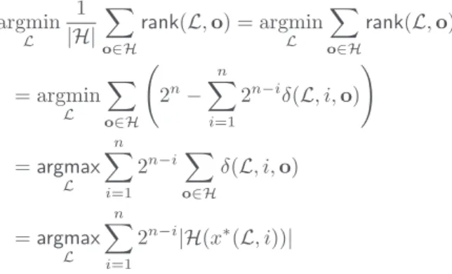
Proof. Given some linear LP-treeL, let X(L, i) be the vari-able at depthi and x∗(L, i) its preferred value. Then
rank(L, o) = 2n− n
#
i=1
2n−iδ(L, i, o)
whereδ(L, i, o) = 1 if o[X(L, i)] = x∗(L, i), 0
argmin L 1 |H| # o∈H rank(L, o) = argmin L # o∈H rank(L, o) = argmin L # o∈H % 2n− n # i=1 2n−iδ(L, i, o) & = argmax L n # i=1 2n−i# o∈H δ(L, i, o) = argmax L n # i=1 2n−i|H(x∗(L, i))|
A linear LP-treeL∗ that maximises this sum must have,
at every leveli, x∗(L∗, i) = argmax
x∈X|H(x)|. And the
rearrangement inequality indicates that the variables must be ordered inL∗in order of decreasing counts|H(x∗(L, i))|,
likewise Algorithm 1.
Learning unconditional lexicographic preferences may be too restrictive, but we do not want to learn fully conditional LP-trees, which would have a size exponential in the number of attributes. One way to learn conditional LP-trees without an exponential number of examples is to consider the num-ber of examples that can be used to continue to induce the tree below a given nodeN : if there is a child N′ofN such
that|H(inst(N′))| is below a fixed threshold τ , then we can
decide not to split; ifH(N′) contains too few examples, it
will not be useful anyway to induce the corresponding part of the LP-tree. We use a function GenerateLabels that im-plements this approach.
Using this thresholdτ , the number of branches of the k-LP-tree learnt is limited because each branch corresponds to at leastτ examples. So there are at most |H|τ branches and
n|H|
τ nodes. In Algorithm 2, at nodeN , one must count the
occurrences inH(inst(N )) of every value of every set of at mostk attributes; this can be done in O(!n
k"d
k|H|), where d
is the maximum domain size of the attributes. The decompo-sition check can be done inO(dk|H|). Furthermore,
Algo-rithm 2 is called for each node. The overall time complexity of the learning algorithm is thenO(n!n
k"d
2k|H|2/τ ).
Pruning
Algorithm 1 returns a treeL that approximately minimizes the empirical expected rank rank(≻L, H) – within the class
of acceptable trees, defined by the chosen threshold. This can lead to overfitting. A standard method to address this problem is to use a score function that trades off, for a given tree, a measure of how well the tree fits to the data with a measure of the complexity of the tree: small mod-els tend to have better generalization properties. We define: Sφ(H, L) = −|H| · rank(≻L, H) − |L| · φ(|H|) where |L|
denotes the size of the model, i.e. the number of its nodes, andφ is a penalty function. In our experiments, we choose φ(|H|) = c, for c a real constant.
Once a LP-tree has been learnt, it can be pruned in or-der to improve its φ-score. This procedure is executed in
a bottom-up fashion. For each non-leaf node N of L, we check whether this node has several outgoing edges. If so, each edge is redirected on the child ofN associated to the preferred value ofX. If the score is improved, we keep this pruned LP-tree; otherwise, we restore the original outgoing edges.
5
Experimental study on randomly
generated data
The first experiments2are run on randomly generated,
reg-ular LP-trees to verify how well a hidden LP-tree can be rediscovered.
LP-tree generation
We randomly generated complete LP-trees (k = 1) with 10 attributes, each having 2 to 6 values (picked with uniform distribution). Each tree was generated in a top-down fashion, starting at the root: at each non-leaf node N , an attribute not already chosen above is picked at random, as well as an order of its values; with probabilityσ, where σ is a split coefficient,N has as many children as X has values; with probability1 − σ, N has a single child.
Given such a randomly picked LP-tree ˘L, we draw a fixed number of outcomes forH using a truncated geometric dis-tribution: the probability of drawing an outcomeo of rank r in ˘L is pµ(r) = Kµ(1−µ)r−1, where1/µ is the mean of pµ.
In the experiments described below, we used a split co-efficientσ = 0.2 and µ was chosen such that the expected value of the drawn rank isX /4: this value (which depends on the sizes that have been picked for the attributes) ensures that, if the root attribute has 2 values, then about 88% of the outcomes are in the preferred subtree.
Results
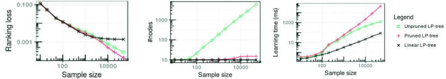
We compared the three variants of the algorithm — LP-Learning without pruning, LP-LP-Learning with pruning and linear LP-Learning — in terms of ranking loss between the hidden and the learnt LP-trees, of size of the learnt tree, and of CPU time necessary to learn the tree (including the prun-ing when used). The splittprun-ing threshold was set toτ = 20 and the penalty function parameterc set equal to 1. Figure 2 shows the results3 for different sample sizes. Each point
represents the mean value on 750 hidden LP-trees.
Figure 2 shows a very good ranking loss. Notice that the ranking loss of linear LP-trees seems to reach a threshold: the hidden LP-trees are not linear, hence the relations they represent are hard to capture with linear structures.
The size of the induced trees increases with the sample size when no pruning is performed, but this size is signifi-cantly reduced by the pruning. This, together with the fact that the ranking loss of the pruned LP-trees is always bet-ter than that of the unpruned LP-trees, suggest an overfitting 2The algorithms have been implemented in Java and have been run on a computer with 8 GB of RAM, a single core 3.4 GHz. Code available at https://github.com/PFGimenez/PhD.
3Because the cardinality of X can be huge, the ranking loss is estimated with a Monte-Carlo sampling with 100,000 samples.
Figure 2: Ranking loss (left), size of the learnt LP-tree (middle) and learning time (right) w.r.t. the sample size.
of the pre-pruning phase. The pruning reduces the size of the learnt LP-tree and enhances its precision, at the cost of a increase in CPU time – that remains sustainable though.
6
Application to value recommendation in
product configuration
The experiments described in this Section are based on a real world problem, car configuration, and the experimental results are drawn for a real world data set, namely a sales history provided by Renault, the French car manufacturer.4
The idea is to use the sales history to build one or several LP-trees, representing the preferences of the past users (the at-tributes in the LP-tree are the configuration variables). These trees can then be used to recommend values during future configurations: given a partial configuration (a partial instan-tiation u∈ U), the LP-tree builds in polynomial time (Lang, Mengin, and Xia 2012) the best (according to the prefer-ence relation it represents) outcome o compatible with u, (i.e. o[U] = u[U]). The system then recommends the value o[X], i.e. the value of X in the preferred completion of u.
Dataset and clustering
We use a dataset that is a genuine sales history containing vehicles of the same type sold by Renault, the French car manufacturer. The vehicles of this data set are described by 48 attributes (mostly binary) and the history contains 27088 items.
This sales history correspond to many customers and there is not enough data to learn the preference relation of each customer (an individual does not often buy a car). How-ever, we can expect clusters of similar users which imply clusters of similar sold products that can be found in the sales history, using some classical k-means algorithm.We can then learn a LP-tree for each cluster, that should approx-imate the preferences of the customers that bought the items in that cluster.
When making a recommendation for a partial outcome u, we use the LP-tree of the cluster that is the nearest to u. This means that, during a configuration session, different LP-trees can be used at different depth in the configuration process. We need to adjust our definition of the empirical mean rank for several LP-trees{Li} and the orders they
rep-resent{≻i}: rank({≻i}, H) = |H|1 $o∈Hminirank(≻i, o)
4Datasets available at http://www.irit.fr/∼Helene.Fargier/ BR4CP/benches.html
Experiment protocol
We use a 10 folds cross-validation protocol. For each item o in the test set, we simulate a configuration session: we start with an empty item u; for each attributeX ∈ X , chosen in a random order, the recommender makes a recommendation ˆ
x given u; we then instantiate X with the value o[X] that has been really chosen by the user; the process is repeated until all attributes have been instantiated. When all items in the test set have been processed, we compute the ratio of accepted recommendations, when the recommended value ˆ
x matched the value o[X] that had been really chosen.
Results
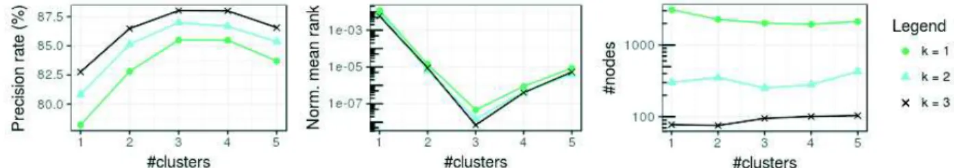
The learning parameterτ is set equal to 20. The results for the learning of unpruned LP-trees are shown in Figure 3. First, we can remark a positive correlation between the pre-cision rate and the normalised empirical mean rank. This suggests that our theoretical score, the mean rank, is indeed correlated with the experimental precision results.
The precision rate ranges from 78.2% (k = 1, 1 cluster) to 88.0% (k=3, 3 clusters); this high precision confirms the practical interest of our approach on real dataset.
The value of the normalised mean rank is in itself inter-esting, because a random LP-tree would have a normalised mean rank equal to 50% while the LP-trees learnt have a normalised mean rank between 1.2% (k = 1, 1 cluster) and 7 · 10−7% (k = 3, 3 clusters).
The precision is maximum for 3 and 4 clusters. While having several clusters increases the expressiveness, each cluster contains fewer examples; this explains the drop in precision with 5 clusters. With more attributes per node (the parameterk) the expressivity is increased, hence a positive impact on the precision.
The size of the model induced (which is the sum of the sizes of the LP-trees learnt for each cluster) seems glob-ally independent of the number of clusters. The effect of the maximum number of attributes per node is stunning, from 2300 nodes withk = 1 to 90 nodes with k = 3. Pruning did not seem to improve results on this dataset.
7
Conclusion and perspectives
This paper constitutes a first approach to the general prob-lem of learning an ordinal preference model from positive examples (and not from pairwise comparisons). We plan to experiment our approach on more real-world datasets. We also plan to study the sample complexity of our algorithms
Figure 3: Precision (left), normalised expected rank (middle) and size (right) of learnt unpruned LP-trees w.r.t. the number of clusters and the maximum number of attributes per nodek.
in a PAC setting since the experiments suggest that the rank-ing loss is inversely proportional to the sample size. An-other lead is the analysis of the computational complexity of finding a LP-tree minimizing the empirical mean rank. In parallel, searching for a scalable and practical algorithm of exact optimization is worth investigating. We also wish to extend the approach to other ordinal preference models like CP-nets; or, more generally, an extension of this framework to partial orders.
References
Booth, R.; Chevaleyre, Y.; Lang, J.; Mengin, J.; and Som-battheera, C. 2010. Learning conditionally lexicographic preference relations. In Proceedings of ECAI’10, 269–274. Boutilier, C.; Brafman, R. I.; Domshlak, C.; Hoos, H. H.; and Poole, D. 2004. CP-nets: A tool for representing and reasoning with conditional ceteris paribus preference state-ments. Journal of Artificial Intelligence Research 21:135– 191.
Br¨auning, M., and H¨ullermeyer, E. 2012. Learning condi-tional lexicographic preference trees. In F¨urnkranz, J., and H¨ullermeyer, E., eds., Proceedings of ECAI’12 Workshop. Br¨auning, M.; H¨ullermeier, E.; Keller, T.; and Glaum, M. 2017. Lexicographic preferences for predictive modeling of human decision making: A new machine learning method with an application in accounting. European Journal of Op-erational Research258(1):295–306.
Braziunas, D. 2005. Local utility elicitation in GAI models. In Proceedings of UAI’05, 42–49.
Brewka, G., et al. 2006. An efficient upper approximation for conditional preference. In Proceedings of ECAI’06, vol-ume 141, 472.
Dombi, J.; Imreh, C.; and Vincze, N. 2007. Learning lexico-graphic orders. European Journal of Operational Research 183:748–756.
Flach, P. A., and Matsubara, E. T. 2007. A simple lexico-graphic ranker and probability estimator. In Proceedings of ECML’07, volume 4701, 575–582.
Fraser, N. M. 1993. Applications of preference trees. In Proceedings of SMC’93, 132–136.
Fraser, N. M. 1994. Ordinal preference representations. The-ory and Decision36(1):45–67.
Freund, Y.; Iyer, R. D.; Schapire, R. E.; and Singer, Y. 2003. An efficient boosting algorithm for combining preferences. Journal of Machine Learning Research4:933–969.
F¨urnkranz, J., and H¨ullermeier, H., eds. 2011. Preference learning. Springer.
Gigerenzer, G., and Goldstein, D. G. 1996. Reasoning the fast and frugal way: Models of bounded rationality. Psycho-logical Review103(4):650–669.
Gonzales, C., and Perny, P. 2004. GAI networks for utility elicitation. In Proceedings of KR’04, 224–234.
Hardy, G. H.; Littlewood, J. E.; and P´olya, G. 1952. In-equalities. Cambridge university press, 2nd edition. Huffman, C., and Kahn, B. E. 1998. Variety for sale: Mass customization or mass confusion? Journal of retail-ing74(4):491–513.
Joachims, T. 2002. Optimizing search engines using click-through data. In Proceedings of SIGKDD’02, 133–142. Koriche, F., and Zanuttini, B. 2009. Learning conditional preference networks with queries. In Proceedings of IJ-CAI’09, 1930–1935.
Lang, J.; Mengin, J.; and Xia, L. 2012. Aggregating conditionally lexicographic preferences on multi-issue do-mains. In Principles and Practice of Constraint Program-ming, 973–987. Springer.
Liu, X., and Truszczynski, M. 2015. Learning partial lex-icographic preference trees over combinatorial domains. In Proceedings of AAAI’15, volume 15, 1539–1545.
Schiex, T.; Fargier, H.; and Verfaillie, G. 1995. Valued con-straint satisfaction problems: Hard and easy problems. In Proceedings of IJCAI’95, 631–637.
Schmitt, M., and Martignon, L. 2006. On the complex-ity of learning lexicographic strategies. Journal of Machine Learning Research7:55–83.
Viappiani, P.; Faltings, B.; and Pu, P. 2006. Preference-based search using example-critiquing with suggestions. Journal of Artificial Intelligence Research27:465–503. Wallace, R. J., and Wilson, N. 2009. Conditional lexico-graphic orders in constraint satisfaction problems. Annals of Operations Research171(1):3–25.
Yaman, F.; Walsh, T. J.; Littman, M. L.; and Desjardins, M. 2008. Democratic approximation of lexicographic prefer-ence models. In Proceedings of ICML’08, 1200–1207.