HAL Id: halshs-03031767
https://halshs.archives-ouvertes.fr/halshs-03031767
Preprint submitted on 1 Dec 2020
HAL is a multi-disciplinary open access
archive for the deposit and dissemination of
sci-entific research documents, whether they are
pub-lished or not. The documents may come from
teaching and research institutions in France or
abroad, or from public or private research centers.
L’archive ouverte pluridisciplinaire HAL, est
destinée au dépôt et à la diffusion de documents
scientifiques de niveau recherche, publiés ou non,
émanant des établissements d’enseignement et de
recherche français ou étrangers, des laboratoires
publics ou privés.
Binary Outcomes and Linear Interactions
Vincent Boucher, Yann Bramoullé
To cite this version:
Working Papers / Documents de travail
WP 2020 - Nr 38
Binary Outcomes and Linear Interactions
Vincent Boucher
Yann Bramoullé
Binary Outcomes and Linear Interactions
†
Vincent Boucher
*and Yann Bramoullé
**November 2020
Abstract
Heckman and MaCurdy(1985) first showed that binary outcomes are compatible with linear econometric models of interactions. This key insight was unduly discarded by the literature on the econometrics of games. We consider general models of linear interactions in binary outcomes that nest linear models of peer effects in networks and linear models of entry games. We characterize when these models are well defined. Errors must have a specific discrete structure. We then analyze the models’ game-theoretic microfoundations. Under complete information and linear utilities, we characterize the preference shocks under which the linear model of interactions forms a Nash equilibrium of the game. Under incomplete information and independence, we show that the linear model of interactions forms a Bayes-Nash equilibrium if and only if preference shocks are iid and uniformly distributed. We also obtain conditions for uniqueness. Finally, we propose two simple consistent estimators. We revisit the empirical analyses of teenage smoking and peer effects of Lee, Li, and Lin (2014) and of entry into airline markets of Ciliberto and Tamer (2009). Our reanalyses showcase the main interests of the linear framework and suggest that the estimations in these two studies suffer from endogeneity problems.
Keywords: Binary Outcomes, Linear Probability Model, Peer Effects, Econometrics of Games.
*Department of Economics, Université Laval, CRREP and CREATE; Email: [email protected] **Aix-Marseille University, CNRS, Aix-Marseille School of Economics; Email: [email protected]
† We thank Habiba Djebbari, Arthur Lewbel, the participants at various seminars and conferences for their helpful
comments, and Aureo de Paula for invaluable feedback. This work was supported by the French National Research Agency Grant ANR-17-EURE-0020.
This research uses data from Add Health, a program directed by Kathleen Mullan Harris and designed by J. Richard Udry, Peter S. Bearman, and Kathleen Mullan Harris at the University of North Carolina at Chapel Hill, and funded by Grant P01-HD31921 from the Eunice Kennedy Shriver National Institute of Child Health and Human Development, with cooperative funding from 23 other federal agencies and foundations. Special acknowledgment is given to Ronald R. Rindfuss and Barbara Entwisle for assistance in the original design. Information on how to obtain Add Health data files is available on the Add Health website (http://www.cpc.unc.edu/addhealth). No direct support was received from Grant P01-HD31921 for this research.
The replication codes are available at https://github.com/vincentboucherecn/linearbinaryinteractions. We usedHlavac(2018) for some of the tables.
1
Introduction
In many contexts, researchers are interested in estimating interactions in agents’ decisions and outcomes. A teenager’s smoking may depend on whether their friends smoke. A firm’s entry into a market may depend on the entry of its competitors. Social and strategic interactions likely play a key role in many important issues, including health, academic achievement, public good provision, consumption and imperfect competition.1 Obtaining credible causal estimates of social and strategic interactions, however, requires addressing some formidable econometric challenges. With binary outcomes, in particular, simultaneity in the behavior of interacting agents may yield multiple equilibria, seeBrock and Durlauf(2001) andTamer(2003). Addressing multiplicity is a central objective of the econometrics of games, surveyed in Bajari, Hong, and Nekipelov
(2013) andDe Paula (2013). In the past 30 years, researchers have made great progress on this issue and have developed econometric frameworks that can, in principle, be used to analyze models with multiple equilibria. The ability to account for multiplicity, however, often comes at a significant cost in terms of practical implementation. At this stage, estimating interactions in binary outcomes under multiplicity may be computationally challenging, may require unrealistic amounts of data and cannot be done while controlling for unobserved heterogeneity with standard fixed effects.
To address these concerns, we propose to revisit linear models of interactions in binary outcomes. Heckman and MaCurdy (1985) showed that binary outcomes are compatible with classical econometric models where an agent’s outcome depends linearly on others’ outcomes. This key insight, however, was discarded by the literature on the econometrics of games,2perhaps because of a belief that these models lack microfoundations. We show that this belief is unfounded and argue that this neglect is undue, given the well-known advantages of linear models. Estimation of linear models is straightforward, they have minimal data requirements, and these models can easily handle fixed effects. Moreover, we show that they can be embedded in models with multiple equilibria. We thus believe that linear models of interactions in binary outcomes should be rehabilitated, even if only as an intermediate step within a deeper analysis.
We consider a general model of linear interactions in binary outcomes. The model notably nests linear-in-means models of peer effects in networks (Bramoullé, Djebbari, and Fortin,2009) and linear models of entry games (Jovanovic, 1989). We develop our analysis in four stages. We first build onHeckman and MaCurdy
(1985) and characterize when this model is well defined (Theorem 1). Errors must have a specific discrete structure, imposed by the binary nature of the outcomes. The model then inherits well-known properties of linear interaction models with continuous outcomes. It generically has a unique solution, and identification is characterized by standard rank conditions, see Wooldridge (2010, Section 9), Bramoullé, Djebbari, and Fortin(2009).
1See, e.g.,Fadlon and Nielsen(2019) on health,Sacerdote(2011) on academic achievement,Foster and Rosenzweig(1995)
on public good provision,Kuhn et al.(2011) on consumption, andBerry(1992) on imperfect competition.
2None of the articles and surveys in our references citeHeckman and MaCurdy(1985) or estimate a linear model of
We then analyze the game-theoretic microfoundations of the econometric model. We adopt standard assumptions of the literature on the econometrics of games but with a different perspective. Most studies in this literature make assumptions on the underlying utilities and preference shocks, and they derive economet-rically relevant implications on the data generating process. In contrast, we start with assumptions on the data generating process—the linear model of interactions—and characterize compatible microfoundations. We consider games of complete and incomplete information. Under complete information, we characterize the preference shocks such that outcomes in the linear model of interactions form a Nash equilibrium of the game with linear utilities. We further derive sufficient conditions for uniqueness in dominant strategies (The-orem 2). Different preference shocks are compatible, and they can notably be independent and continuously distributed. In the presence of multiple equilibria, we show that outcomes in the linear model of interactions form the only Nash equilibrium robust to increases in shock dispersion (Proposition 1). Under incomplete information, we show that under independence, outcomes in the linear model of interactions form an interior Bayes-Nash equilibrium of the game with linear utilities if and only if preference shocks are iid and uniformly distributed. Furthermore, this is the unique Bayes-Nash equilibrium under moderate interactions (Theorem 3). Overall, our results provide game-theoretic microfoundations for the linear model of interactions in binary outcomes.
Our analysis highlights the importance of distinguishing between two types of stochastic terms: errors, defined from the data generating process, and preference shocks, appearing in underlying microfoundations. The binary nature of the outcomes imposes strong restrictions on the data generating process. Reduced-form errors are always binary, and, in our context, structural errors are discrete. Preference shocks are not subject to these restrictions, however, and are generally not identified without further assumptions. Thus even with linear utilities, many different preference shocks are generally compatible with the data generating process.
In a third stage, we propose two simple estimators to analyze interactions in binary outcomes on real data, which are consistent in a many-groups asymptotic framework. One is a classical Two-Stage Least Squares (2SLS), the other is a Nonlinear Least Squares (NLS) exploiting the structure of reduced-form equations. We discuss the estimators’ properties and compare their small-sample performances through Monte Carlo simulations. The NLS appears to be more efficient. Including fixed effects in a NLS estimation may be problematic, however, due to the incidental parameter problem. By contrast, eliminating group-level unobservables through within-group deviations is standard in 2SLS estimations, and hence the 2SLS may be preferred, in practice, for most applications.
Finally, we analyze real data with our proposed linear framework. To highlight differences with existing approaches, we revisit two studies: Lee, Li, and Lin(2014) on peer effects in teenage smoking andCiliberto and Tamer (2009) on entry into airline markets. We reanalyze the same data as in the original studies and assess the robustness of the original results. These reanalyses illustrate the main advantages of the linear framework: ease of implementation, the availability of overidentification tests, and the ability to handle fixed effects. In contrast, existing nonlinear frameworks are generally computationally demanding, lack
overidentification tests, and cannot handle large sets of fixed effects. In Lee, Li, and Lin (2014), we can include fixed effects at the school-grade level, a natural feature missing from the original analysis. With or without these fixed effects, linear estimates of endogenous peer effects are positive and significant, as observed in the original study. The joint validity of the instruments is, however, strongly rejected by overidentification tests.
For Ciliberto and Tamer (2009), we can include airline fixed effects, which were also absent from the original analysis. Results from our reanalysis are qualitatively different from the original results. Estimates of strategic interactions between airlines are generally positive and significant in a linear framework, whereas they are negative and significant in Ciliberto and Tamer (2009). Absent a proper means of testing one specification versus another, we can only speculate on the causes behind these differences.3 As in many studies in the econometrics of games, the first step of Ciliberto and Tamer (2009)’s estimation method is to obtain nonparametric estimates of conditional choice probabilities. These estimates capture how the probabilities of all possible market outcomes depend on all covariates. The estimation of conditional choice probabilities suffers from a well-known curse of dimensionality in practice, seeAndrews, Berry, and Barwick
(2004). This problem appears to be severe in Ciliberto and Tamer(2009)’s application, as researchers must obtain nonparametric estimates of 63 functions of 20 variables with only 2, 742 observations. In contrast, estimates of conditional choice probabilities are not required to estimate linear models. More generally, linear estimations are not affected by a curse of dimensionality, and we suspect this plays an important role in explaining the different results. In addition, the joint validity of the instruments is also strongly rejected by overidentification tests. This suggests that the original analyses ofLee, Li, and Lin(2014) andCiliberto and Tamer(2009), as well as our reanalyses, suffer from endogeneity problems.
Our analysis contributes, first, to a large and still-expanding literature on peer effects.4 Early studies focused on group interactions. Population is then partitioned into groups; agents interact with all other members of their group and with no members of another group. Brock and Durlauf (2001) first proposed a microfounded econometric framework to analyze peer effects on binary outcomes. They consider a setup of incomplete information under group interactions. They show that the model has a unique equilibrium under moderate interactions and multiple equilibria under strong interactions. Soetevent and Kooreman
(2007) analyze peer effects on binary outcomes under complete information and group interactions. They find that the game typically has a large number of equilibria. They propose a simulated maximum likeli-hood estimator based on the assumption that all Nash equilibria are equally likely. Nakajima (2007) also analyzes peer effects on binary outcomes under complete information and group interactions. He considers a stochastic Markov process where agents sequentially and myopically play a best response. He assumes that the likelihood function is equal to the steady-state distribution of this process. Recent studies consider more
3Ciliberto and Tamer(2009) develop and implement a partial identification approach. Although no direct specification tests
are available, measures of goodness of fit are quantitatively similar across the two specifications, with a slight advantage to the linear models.
complex network interactions.5 Li and Zhao(2016) adapt partial identification approaches under complete information to the analysis of peer effects in networks and binary outcomes. Lee, Li, and Lin (2014) extend the incomplete information framework ofBrock and Durlauf(2001) to networks. They show that uniqueness holds under moderate interactions and propose an iterative simulated maximum likelihood estimator based on a subroutine that repeatedly computes the solution of a high-dimensional nonlinear fixed-point system. All these studies develop nonlinear frameworks to analyze peer effects on binary outcomes.
In contrast, we show that linear models of peer effects, traditionally used to study continuous outcomes (Manski (1993)), can also be used for binary outcomes. We show that these models can be given proper microfoundations and maintain key properties when applied to binary outcomes. This concerns, in particular, the identification results and ideas of Bramoullé, Djebbari, and Fortin (2009), which exploit holes in the network structure to solve the reflection problem.6 We revisit the empirical analysis of peer effects and teenage smoking ofLee, Li, and Lin(2014). We obtain similar estimates of endogenous peer effects through a much simpler estimation procedure. In addition, we can control for school-grade fixed effects and verify whether the network-based instruments pass overidentification tests, two features absent from the original study.
Our analysis contributes, more generally, to the literature on the econometrics of games. Since the early work of Jovanovic (1989) and Bjorn and Vuong (1997), researchers have made great progress on the empirical analysis of models with multiple equilibria. Applied researchers who wish to estimate interactions in binary outcomes under multiplicity can, notably, specify a flexible selection mechanism dependent on estimated parameters (Bajari, Hong, and Ryan,2010), adopt a partial identification approach under complete information (Ciliberto and Tamer,2009), or assume that the same equilibrium is played across games under incomplete information (Aguirregabiria and Mira, 2007). Preference shocks are generally assumed to be logistically or normally distributed. Different assumptions yield different nonlinear econometric frameworks; a common first step is often to obtain flexible estimates of conditional choice probabilities. Despite this important methodological progress, however, two features may limit the usefulness of these approaches for obtaining credible causal estimates. First, and depending on the context, econometric frameworks developed to handle multiplicity may have unrealistic data requirements. We argue that this applies to the application in
Ciliberto and Tamer(2009). Second, introducing unobserved heterogeneity in these frameworks is generally impractical or unfeasible. Due to the incidental parameter problem, nonlinear estimators usually cannot handle fixed effects, whose numbers grow at the same rate as sample size. While they could, in principle, account for a finite number of fixed effects, their introduction further intensifies the data requirements.7
5About 10 years ago, four studies independently understood that the reflection problem (Manski(1993)) is naturally solved
by network interactions (Bramoullé, Djebbari, and Fortin(2009), De Giorgi, Pellizzari, and Redaelli(2010),Lin(2010), and
Laschever(2013)). Since then, the literature on peer effects in networks has rapidly grown and extended in many directions, seeBoucher and Fortin(2015),De Paula(2017), andBramoullé, Djebbari, and Fortin(2020). Relatively few studies, however, analyze peer effects in networks and binary outcomes.
6The linear framework can also, of course, be applied to analyze peer effects in binary outcomes with group interactions,
under appropriate identification conditions. For instance,Soetevent and Kooreman(2007) and Nakajima(2007) assume that an agent’s outcome does not depend directly on their peers’ characteristics (no contextual peer effects). We can easily estimate linear interaction models of their data under the same assumption.
To help reconcile the structural and reduced-form approaches, we propose to rehabilitate linear models of interactions in binary outcomes. While linear models cannot account for multiplicity, they provide a natural benchmark. They are very easy to implement, have minimal data requirements, and can easily handle fixed effects. They have transparent identification conditions and well-understood overidentification tests. Heckman and MaCurdy(1985) first showed that classical linear models of simultaneous equations are compatible with binary endogenous variables. We build on this early work8 and provide the first systematic analysis of the game-theoretic microfoundations of linear models of interactions. We show that they can be obtained as equilibria of games of complete or incomplete information with linear utilities and we characterize compatible preference shocks. Preference shocks can be independent and continuously distributed under complete information and iid and uniformly distributed under incomplete information. Discarding linear models of interactions simply because they do not emerge as equilibria of game-theoretic models with logistic or normal preference shocks seems rather extreme. Microfoundations and preference shocks are, in any case, not identified from the data generating process without making strong assumptions. We thus believe that linear models have a legitimate place in the toolkit of applied researchers interested in interactions in binary outcomes.
Finally, our analysis contributes to the literature on the econometrics of discrete variables and on linear probability models in particular. Researchers hold diverse views on the use of linear models to analyze binary outcomes. Following Angrist and Pischke (2008), applied economists focused on obtaining credible causal estimates generally estimate linear probability models. In contrast, researchers who are more theoretically or methodologically oriented often adopt models based on latent variables. This preference is perhaps explained by a belief that linear probability models lack microfoundations. This belief is incorrect. Heckman and Snyder Jr (1997) provide microfoundations for linear probability models with a single decision-maker. A main contribution of our analysis is to clarify the game-theoretic microfoundations of linear probability models with outcome interactions. Notably, we show that linear models of interactions in binary outcomes are particular cases of models with latent variables. Given the many advantages of a linear framework, we believe that it could become a natural benchmark in empirical studies of binary outcome interactions.
The paper proceeds as follows. We present the econometric framework in Section 2 and analyze its microfoundations in Section 3. We propose estimators and discuss their properties in Section 4. We revisit existing studies of interactions in binary outcomes in Section 5 and conclude in Section 6.
2
Econometric framework
A researcher has data on n agents and analyzes interactions affecting a binary outcome. Let yi∈ {0, 1} denote
agent i’s outcome. Let y ∈ Rn denote the vector of outcomes and x a matrix containing all observables.
heterogeneity when the unobservables have finite support. This is a potentially promising result. Its empirical applicability has not yet been demonstrated, however, and the assumption of finite support represents, in any case, a significant restriction.
For any well-defined data generating process on (x, y), we find it useful to distinguish between two types of stochastic terms. By convention, errors are defined directly from the data generating process, whereas preference shocks appear in underlying microfoundations. We define reduced-form errors as νi= yi− E(yi|x),
leading to yi= E(yi|x) + νi and E(νi|x) = 0.
As is well known, the binary nature of the outcome imposes strong restrictions on the data generating process. In particular, P(yi= 1|x) = E(yi|x), and the reduced-form error νi is a binary, Bernouilli stochastic
variable: νi= 1 − E(yi|x) with probability E(yi|x) and −E(yi|x) with probability 1 − E(yi|x).9 Thus, while
preference shocks are often assumed to be continuously distributed, reduced-form errors are always binary. For instance, consider a probit model without interactions. Let 1(Yi ≥ 0) = 1 if Yi > 0 and 0 if Yi < 0.
Then, yi=1(xiγ + ei ≥ 0), and preference shock ei follows a normal distribution N (0, 1) with cdf Φ, while
reduced-form errors are such that νi = 1 − Φ(xiγ) with probability Φ(xiγ) and −Φ(xiγ) with probability
1 − Φ(xiγ).
In our analysis, we consider the following general model of linear interactions
yi= fi(x, θ) +
X
j
βijyj+ εi, (1)
under the exogeneity assumption, E(εi|x) = 0. Outcome yiis affected by observables through function fiand
parameters θ and by others’ outcomes through linear interactions P
jβijyj. Let β denote the interaction
matrix, where βii= 0, and βij can potentially have any sign.
Whether there exists an error structure such that equation (1) holds with binary outcomes is not imme-diate. The interaction term P
jβijyj can take up to 2n−1 values and partly determines yi, which can take
only 2 values. In this Section, we clarify the conditions under which this model is well defined. We analyze underlying microfoundations in the next Section.
Model (1) nests two important cases of interactions in binary outcomes: peer effects and entry games. First, consider the benchmark linear-in-means model of peer effects in networks, see Bramoullé, Djebbari, and Fortin (2009). For each agent i, the researcher observes characteristics xi and set of peers Ni. Peer
relationships form a binary directed network. Let di= |Ni| denote i’s degree, i.e., the number of peers of i.
Assume that no agent is isolated, di> 0.10 Define G as the linear-in-means matrix of interactions: gij= d1i
if j ∈ Ni and 0 otherwise. The linear-in-means model of peer effects in networks can be written as
yi= α + xiγ + X j gijxjδ + β X j gijyj+ εi, (2)
under the assumption that E(εi|x, G) = 0. In this model, outcomes can be affected by individual
characteris-tics (individual effects, γ), peers’ characterischaracteris-tics (contextual peer effects, δ), and peers’ outcomes (endogenous peer effects, β). Model (2) is a case of model (1) with θ = (α, γ, δ), fi(x, G, θ) = α + xiγ +Pjgijxjδ, and
9
This further implies that V(yi|x) = E(yi|x)(1 − E(yi|x)). The conditional variance and, more generally, higher moments of
the conditional outcome distribution do not contain extra information with respect to the conditional expectation.
the interaction matrix β = βG. In this model, the structure of the interactions G is known but not their extent, β.
The assumption E(εi|x, G) = 0 means that characteristics and the network are strictly exogenous and
the problem of correlated effects has been solved.11 This framework has generally been applied to study continuous outcomes. We show below that it is also compatible with binary outcomes.
Our second main application is about entry games. These games have been introduced to study competi-tion between a small number of firms in a large number of markets. Firm i’s decision to enter market m may depend on characteristics of the firm and the market and on the entry decisions of its competitors. In the literature, researchers generally consider nonlinear models of entry games, e.g.,Ciliberto and Tamer(2009). In contrast, we consider the following linear model. Let yim∈ {0, 1} denote the entry of firm i into market
m. Then,
yim= α + ximγ + zmλ +
X
j
βijyjm+ εim, (3)
under the assumption that E(εim|x, z) = 0.12 Firm i’s entry depends on firm-market characteristics xim, on
market characteristics zm, and on other firms’ entriesPjβijyjm. Observe that model (3) is a case of model
(1) applied to firm-market observations with θ = (α, γ, λ), fim(xim, zm, θ) = α + ximγ + zmλ, and under
the assumption that the interaction matrix β is constant across markets.
We now characterize when binary outcomes are compatible with linear interactions, following arguments in
Heckman and MaCurdy(1985). In what follows, the notation x refers to a matrix containing all observables, including the network in a peer-effect application and market characteristics in an entry game. Note that equation (1) defines a fixed-point system in the outcome profile y. In matrix notations,
y = f + βy + ε.
We assume that the matrix I−β is invertible. This holds generically and implies that this system has a unique solution. The reduced form of model (1), expressing outcomes y as a function of observables, parameters and errors is equal to
y = (I − β)−1f + (I − β)−1ε.
Let Pi= [(I − β)−1f ]i and νi = [(I − β)−1ε]i. Here, Pi= E(yi|x) = P(yi= 1|x) is the conditional expected
outcome and hence must lie between 0 and 1. Then, νi= yi− E(yi|x) is the reduced-form error of the data
generating process.
We have yi = Pi+ νi, and yi = 1 and νi = 1 − Pi with probability Pi, while yi = 0 and νi = −Pi with
probability 1 − Pi. Then, ε = (I − β)ν, leading to our first result.
11Bramoullé, Djebbari, and Fortin(2020) show that exogeneity of either a characteristic or the network can be sufficient to
identify peer effects in model (2).
12Nonlinear models of entry games generally assume that y∗
im= α + ximγ + zmλ +Pjβijyjm+ eim, where yim∗ is a latent
Theorem 1. Assume that I − β is invertible and that ∀i, Pi= [(I − β)−1f ]i∈ [0, 1]. Outcomes in the unique
solution to model (1) are binary, yi ∈ {0, 1}, if and only if
εi= νi−
X
j
βijνj,
where νi= −Pi with probability 1 − Pi and 1 − Pi with probability Pi.
Theorem 1 clarifies the conditions under which binary outcomes are compatible with linear interactions. The structural errors appearing in model (1) must have a specific discrete structure, induced by the binary nature of the outcomes and the linear framework. Note that these structural errors depend directly on the data generating process. In the next Section, we analyze the microfoundations of model (1) and find that preference shocks in underlying microfoundations can have very different properties. For instance, they can be iid and continuously distributed, see Theorem 3.
As in any data generating process with binary outcomes, reduced-form errors are binary and generally depend on observables and parameters. They can be correlated, and possible correlation patterns also depend on observables and parameters.13 In the absence of interactions and when fi is linear, model (1) reduces to
a standard linear probability model. In the presence of interactions, structural errors εi usually take more
than two values. In general, εi can take up to 2n values. Structural errors are also correlated even when
reduced-form errors are uncorrelated. In model (2) of peer effects in networks, εican take up to 2di+1values.
Denote d(i, j) as the distance between i and j in the network, i.e., the number of links in a shortest path connecting i to j (or ∞ if there is no path connecting i to j). Then, εiand εjare generally correlated if i and j
are peers or peers of peers. In contrast, cov(εi, εj) = 0 if d(i, j) > 2 and reduced-form errors are uncorrelated.
Thus, the stochastic structure of structural errors generally depends on the network of interactions.
Probabilities must of course lie between 0 and 1. This is guaranteed in model (1) with binary outcomes when for any i, [(I − β)−1f ]i ∈ [0, 1]. This condition depends both on interactions β and expected outcomes
absent of interactions f . For instance, when n = 2 and f1, f2 ∈]0, 1[, it holds for moderate interactions
of any sign and for large negative interactions.14 Moreover, in any application we can easily compute the proportion of observations for which the estimated probability lies between 0 and 1. As with the standard linear probability model, this provides a simple measure of whether the estimated model is appropriate. We report these proportions in our estimations in Section 5.
A key property of the linear framework is that if I − β is invertible, there is a unique solution to the fixed-point system defined by model (1). In other words, the econometric model is both coherent and complete, see
Tamer(2003) andLewbel(2019). In contrast, almost all existing studies of interactions in binary outcomes rely on a latent variable model of the following kind:
13For instance, one possible stochastic structure with correlation is as follows. Suppose that u is uniformly distributed on
[0, 1], and for every i set νi= 1 − Piif u < Piand −Piif u > Pi.
14Note that for (almost) any β and p ∈ [0, 1]n, the system (I − β)−1f = p always has a unique solution f . Thus, the condition
yi=1(fi(x, θ) − 1 2 + X j βijyj+ ei≥ 0). (4)
The econometric model defined by equation (4) is generally incoherent or incomplete. The fixed-point system can have multiple solutions, leading to an incomplete model. The fixed-point system can also have no solution, leading to an incoherent model. Interestingly, we show in the next Section that linear model (1) is a particular case of latent variable model (4) for specific assumptions on preference shocks ei.
Furthermore, identification in a linear framework follows from well-known results. For the linear-in-means model of peer effects in networks, in particular, the identification results of Bramoullé, Djebbari, and Fortin
(2009) apply when outcomes are binary under the assumptions of Theorem 1. This holds because their analysis does not impose restrictions on the nature of the outcome or on the error terms, other than the exogeneity assumption E(εi|x, G) = 0.
Corollary 1. (Bramoullé, Djebbari, and Fortin,2009) Consider the linear-in-means model of peer effects in networks with binary outcomes and under the assumptions of Theorem1. Assume δ + βγ 6= 0. The model is identified if the matrices I, G, and G2 are linearly independent.
Identification notably holds when the network’s diameter is greater than or equal to 2 or under group interactions when groups have different sizes.
With entry games, model (3) is generally identified when the entry of firm i is affected by some firm-market characteristic xim that does not directly affect the entry of other firms, a standard assumption in
the literature. The entry of firm j can then be instrumented by xjm in equation (3), see e.g.,Bajari, Hong,
and Nekipelov(2013). More generally, model (1) defines simultaneous linear equations in outcomes. When the functions fi are also linear, classical rank conditions for identification apply, see e.g.,Wooldridge (2010,
Section 9).
3
Microfoundations
We now analyze the microfoundations of model (1). We assume in this Section that the outcome yi∈ {0, 1}
is a choice of agent i. We consider games of complete or incomplete information under the assumptions of Theorem1 that I − β is invertible and Pi= [(I − β)−1f ]i∈ [0, 1].
We adopt standard assumptions of the literature on the econometrics of games. We consider a classical random utility framework (McFadden, 1974). Agent i derives utility vi(yi, y−i) from playing yi when other
agents play y−i. Utility vi(yi, y−i) is the sum of deterministic utility ui(yi, y−i) and of preference shock
ei(yi). Let ∆ui(y−i) = ui(1, y−i) − ui(0, y−i) denote the relative deterministic utility of playing 1, and
let ei = ei(1) − ei(0) denote the relative preference shock in the utility of playing 1. Under complete
information, the deterministic utilities and preference shocks of all agents are common knowledge. Under incomplete information, the deterministic utilities of all agents and the distribution of preference shocks are
common knowledge. Agent i observes the realization of her own shock ei but not the realization of others’
shocks e−i.
Existing studies of interactions in binary outcomes generally assume that relative utility is linear in others’ actions: ∆ui(y−i) = fi− 1 2 + X j βijyj. (5)
Interestingly, linear relative utility (5) is consistent with quadratic utility ui(yi, y−i) = yifi−12y 2 i+
P
jβijyiyj.
This quadratic utility has been well studied in network games with continuous actions, see Ballester, Calvó-Armengol, and Zenou (2006) and Bramoullé, Kranton, and D’amours (2014), and has been proposed as a microfoundation of the econometric model of peer effects with continuous outcomes, see e.g., Davezies, d’Haultfoeuille, and Fougère (2009). This provides a common game-theoretic framework for binary and continuous action games.
3.1
Complete information
Under complete information, outcomes y are assumed to form a Nash equilibrium of the game for any realization of preference shocks e. This means that for every agent i, if yi = 1 then ∆ui(y−i) + ei ≥ 0,
whereas if yi = 0 then ∆ui(y−i) + ei ≤ 0. Therefore, yi = 1(∆ui(y−i) + ei ≥ 0), and the system of
equilibrium conditions is equivalent to a latent variable model with interactions, such as (4).
An important early finding is that multiple equilibria necessarily appear in games of complete information with linear relative utility when interactions are positive and preference shocks have full support over R, see Tamer (2003) and De Paula (2013). To see why, consider the linear relative utility (5). Note that vi(1, 0) − vi(0, 0) = fi−12+ ei. Then, (0, 0, ..., 0) is an equilibrium iff for every i, ei≤ −(fi−12). Similarly,
vi(1, 1)−vi(0, 1) = fi−12+Pjβij+ei, and (1, 1, ..., 1) is an equilibrium iff for every i, ei≥ −(fi−12)−Pjβij.
Therefore, both 0 and 1 are Nash equilibria iff for every i, −(fi−12) −Pjβij ≤ ei ≤ −(fi−12). If for every
i,P
jβij > 0 and the density of eiis everywhere strictly positive, then there is a strictly positive probability
of multiple Nash equilibria. Multiplicity appears when preference shocks take intermediate values.
As our second main result, we characterize when the linear model of interactions can be microfounded with linear relative utilities. More precisely, denote by y∗ the unique solution to equation (1) under the conditions on parameters and errors described in Theorem1. We provide necessary and sufficient conditions on preference shocks under which y∗ is a Nash equilibrium of the game with linear relative utilities and sufficient conditions under which this is the unique Nash equilibrium in dominant strategies.
Theorem 2. The unique solution to the linear model of interactions (1) is a Nash equilibrium of the game with linear relative utilities (5) and preference shocks ei if and only if
It is the unique Nash equilibrium in dominant strategies if
νi> 0 ⇒ ei>12− Pi−Pjβijνj+Pj|βij| and νi< 0 ⇒ ei< 12− Pi−Pjβijνj−Pj|βij|.
Theorem 2 describes precisely how preference shocks must be related to reduced-form errors in game-theoretic microfoundations to model (1). Intuitively, preference shocks must be large enough in situations where the agent plays 1 and low enough in situations where the agent plays 0. Theorem 2 has several noteworthy implications.
First, it shows that the linear model of interactions (1) is a particular case of the model with latent variables (4). When preference shocks satisfy the first set of inequalities described in Theorem2, the linear model corresponds to one solution of the system of equations defined by model (4) among many possible solutions. When preference shocks satisfy the second set of inequalities, however, the linear model corresponds to the unique solution and hence the two models are formally equivalent.
Second, it shows that preference shocks in underlying microfoundations are not identified without further assumptions. Thus, very different kinds of preference shocks are consistent with the econometric model. The linear model of interactions can notably be microfounded with preference shocks that are discrete and correlated, like structural errors, or independent and continuously distributed. To see why, note first that structural errors actually provide admissible preference shocks.15 However, underlying preference shocks can also be independent and continuously distributed. For instance, consider a situation where the νi’s are
uncorrelated. Assume that eiis uniformly distributed on [−Li− 1 + Pi, −Li] ∪ [Mi, Mi+ Pi], that the ei’s are
independent, and that νi=1(ei ≥ 0) for Li, Mi≥ 12 + 2Pj|β|ij. A direct application of Theorem 2 shows
that in this case, the unique solution to the linear model of interactions is the unique Nash equilibrium of the corresponding game.
A third implication is that, in some cases, the unique solution to the linear model of interactions is the unique Nash equilibrium in dominant strategies. This happens when preference shocks are sufficiently dispersed: sufficiently high when high and sufficiently low when low. Preference shocks then do not take intermediate values, bypassing the multiplicity domain.
An intriguing consequence is that even in the presence of multiple Nash equilibria, the linear model of interactions becomes the unique equilibrium following specific changes in preference shocks. The linear model of interactions is then, in a sense, the only robust Nash equilibrium. We next develop these arguments formally. In our next result, we show that this reasoning holds for any deterministic utility and preference shocks.
Proposition 1. Suppose that the unique solution to model (1) is a Nash equilibrium of the game of complete information with deterministic utilities Ui and preference shocks ei. Consider preference shocks e0i where
e0i= ei+ Mi if νi> 0 and ei− Li if νi < 0 and Li, Mi≥ 0. Then, the unique solution to model (1) remains
15A direct application of Theorem2shows that when e
i= εi, the unique solution to model (1) is always a Nash equilibrium
of the corresponding game and is the unique Nash equilibrium in dominant strategies when ∀i,P
a Nash equilibrium of the game of complete information with deterministic utilities Ui and preference shocks
e0i, and it is the unique Nash equilibrium in dominant strategies when Li and Mi are sufficiently large.
Proposition1 formalizes a natural idea: increasing preference shocks in situations where the agent plays 1 and decreasing preference shocks in situations where the agent plays 0 can only increase the incentives to play these actions. Because of the discreteness of the strategy space, we further show that these heightened incentives yield dominant strategies when these increases and decreases are sufficiently high. Say that a Nash equilibrium y for preference shocks e is robust to increases in shock dispersion when y remains an equilibrium for preference shocks e0i where e0i= ei+ Li if νi> 0 and ei− Mi if νi< 0 and Li, Mi ≥ 0.16
Corollary 2. Suppose that the unique solution to model (1) is a Nash equilibrium of the game of complete information with deterministic utilities Ui and preference shocks ei. Then, this is the unique equilibrium
robust to increases in shock dispersion.
To summarize, outcomes in the linear model of interactions correspond to a Nash equilibrium of a game of complete information with linear relative utilities under conditions on preference shocks, which we charac-terize. These preference shocks are not identified and could be, for instance, independent and continuously distributed. Furthermore, outcomes in the linear model correspond to the unique Nash equilibrium that is robust to increases in shock dispersion. Together, these results provide game-theoretic microfoundations to the linear model of interactions under complete information. We next look at incomplete information.
3.2
Incomplete information
Under incomplete information, agent i observes her preference shock eibut not others’ shocks e−i. Outcomes
y are assumed to form a Bayes-Nash equilibrium of the game.
A first remark is that when actions are dominant under complete information, they are also dominant under incomplete information. Therefore in situations described in Theorem 2 and Proposition 1, where uniqueness in dominant strategies holds under complete information, the corresponding game of incomplete information also has a unique Bayes-Nash equilibrium in dominant strategies. As shown above, these results involve preference shocks with a dispersed distribution and non-convex support. This raises the question of whether shock dispersion and support non-convexity are necessary in microfoundations of the linear model of interactions.
In our third main result, we show that these features are not necessary. Under incomplete information and when reduced-form errors are uncorrelated, the linear model of interactions can be microfounded with preference shocks that are iid and uniformly distributed over an interval. Moreover, if preference shocks are independent between agents and independent of observables, they must be uniformly distributed.
16There exists an extensive game-theoretic literature on robust equilibria, proposing various definitions of robustness. A
common, central idea, as here, is that an equilibrium is robust when it remains an equilibrium following perturbations of the underlying game (e.g., Trembling Hand perfection,Selten(1975)).
Theorem 3. Assume that reduced-form errors νi are uncorrelated. Consider the game of incomplete
infor-mation with linear relative utilities (5) and preference shocks ei with ei⊥ e−i, x. The unique solution to the
linear model of interactions (1) is the unique interior Bayes-Nash equilibrium for all possible β, f if and only if the ei’s are iid and uniformly distributed over [−12,12]. If in addition ∀iPj|βij| < 1, this is the unique
Bayes-Nash equilibrium.
Our proof in Appendix relies on the well-known property that a uniform distribution is the only distribu-tion with a linear cumulative density funcdistribu-tion.17 The uniqueness condition comes from a classical contraction mapping argument,18and we show in Appendix that the game can have multiple Bayes-Nash equilibria when this condition is not satisfied. The uniqueness condition is easy to verify for estimated parameters, and we will see that it always holds in the empirical applications in Section 5. The fact that uniqueness holds under incomplete information when interactions are moderate is well known, see e.g., Brock and Durlauf (2001) andLee, Li, and Lin(2014). However, existing applications typically assume that preference shocks have full support, thereby leading to nonlinear econometric models. For instance,Lee, Li, and Lin (2014) consider a logit framework, see Section 5.1. Theorem3clarifies the conditions under which a linear model of interactions in binary outcomes can be obtained as a Bayes-Nash equilibrium of a game of incomplete information.
4
Estimators
In this Section, we propose two simple estimators to analyze data with binary outcomes generated by model (1). We consider a many-groups asymptotic framework with independent groups of bounded size. This corresponds to a many-network asymptotic in a peer effect setting19or to a many-market asymptotic for entry games. The number of groups thus goes to infinity with sample size, and consistency and the asymptotic normality of extremum estimators are guaranteed under standard assumptions, see, e.g.,Cameron and Trivedi
(2005), Section 5.3.20 We explore the small sample properties of our proposed estimators through Monte Carlo simulations and apply these estimators to real data in Section 5.
We consider the following variant of model (1). We assume that f is linear in observables and that the interaction matrix β depends linearly on a fixed number of parameters to estimate. Formally, f = Xθ and β =PK
k=1βkGk, where K is finite and independent on the sample size. This yields
y = Xθ +
K
X
k=1
βkGky + ε. (6)
While not essential, the linearity of f is sufficient for most applications and facilitates exposition. The
17Unexpectedly, our proof is quite similar to the proof of Proposition 3.2 inBloch and Quérou(2013) in a context of monopoly
pricing under network externalities.
18We show in Appendix that uniqueness holds when kβk < 1 for any submultiplicative matrix norm k · k.
19Population is then partitioned into groups, and agents can only be affected by others in their own group. The overall
network is composed of disjoint subnetworks with a block diagonal interaction matrix.
20The analysis of estimators’ properties in a single network asymptotic framework is an active area of research, see e.g.,Lee
assumption on the interaction matrix ensures that the number of parameters to estimate does not grow with sample size21 and allows us to provide a common framework for our two applications. Denote by β(K)= (β1, ..., βK) and similarly for G(K).
In the benchmark linear-in-means model of peer effects in networks, there is only one interaction parameter to estimate. In that model, K = 1 and β = βG, where Gij = 1/di if i and j are linked and 0 otherwise.
Extended versions of the model with heterogeneous peer effects, as in Nakajima (2007), Soetevent and Kooreman (2007), and Dieye and Fortin (2017), are also cases of model (6). For instance, when men and women can be differentially affected by their male and female peers, there are K = 4 interaction parameters to estimate. In that case, β = βF FGF F+ βF MGF M+ βM MGM M+ βM FGM F, where, for example, GF M
models the structure of interactions between female individuals and male peers.
In the linear model of entry game, there are K = n(n − 1) interaction parameters to estimate, where n is the number of firms competing across markets. Here, β = P
i,jβijGij, where Gij has 1 at entry (i, j)
and 0’s elsewhere. In the next Section, we estimate a version of this model where the entry of a firm has a common impact on the entry of other firms, i.e., βij = βj. In that version, there are K = n parameters to
estimate, and β =PN
j=1βjGj, where Gj=PiGij has 1’s in its jth column and 0’s elsewhere.
We assume that the model to be estimated is identified, see Section 2. The linear-in-means model of peer effects is identified under conditions reported in Corollary1. Similar conditions hold when peer effects are heterogeneous, see e.g., Dieye and Fortin (2017). In the linear model of entry games, identification holds under the exclusion restrictions that some characteristics of firm j, affecting its profit, do not affect the profit of firm i.
Our first proposed estimator is a Two-Stage Least Squares (2SLS) estimator, building on the 2SLS es-timation strategies proposed by Kelejian and Prucha (1998) and Bramoullé, Djebbari, and Fortin (2009). Since E(ε|X, G(K)) = 0, we have
E(Gky|X, G(K)) = GkXθ + K
X
l=1
βlGkGl(I − β)−1Xθ.
In particular, variables in GkX that are not already in X provide natural instruments for Gky in equation
(6).
In the linear-in-means model (2), we have X = [1, x, Gx] and hence GX = [G1, Gx, G2x], so G2x can be used as an instrument for Gy. This instrument is valid under the conditions described in Corollary
1. Intuitively, characteristics of peers of peers who are not peers affect individual outcome only through their impact on peers’ outcomes, see Bramoullé, Djebbari, and Fortin (2009). In the linear model of entry game (3), for any market m, we have Xm= [1, xm, zm] and, hence, GijXm= [Gij1, Gijxm, Gijzm]. Here,
[Gijy]i= yj can be instrumented by [Gijxm]i= xjm. The impact of the entry of firm j on i’s entry can be
instrumented by the characteristics of firm j.
21Peng(2019) proposes a penalized regression strategy that depends on the weaker assumption that K ≤ c√n
ln n for some c as
The validity of this IV strategy relies on the exogeneity condition E(εi|X, G(K)) = 0 but not on the
specific structure of the errors. This strategy is thus valid when errors have the discrete structure uncovered in Theorem1. Error structure may of course matter for inference. In particular, errors in the linear-in-means model (2) with binary outcomes are heteroscedastic and correlated among peers and peers of peers, see Section 2. In a many-groups asymptotic framework, we propose to use group-level cluster-robust standard errors for inference since they allow for arbitrary within-group correlations, see Cameron and Miller(2015). In other asymptotic frameworks, spatial Heteroscedastic and Autocorrelation Consistent (HAC) variance estimators could be appropriate (e.g.,Conley (1999),Kelejian and Prucha(2007),Leung(2019)).22
Our second proposed estimator is a Nonlinear Least Squares (NLS) estimator, exploiting the struc-ture of the reduced-form equations. Recall that yi = Pi+ νi with E(νi|x) = 0, and P(β(K), θ) = (I −
PK
k=1βkGk)−1Xθ. The model can thus be consistently estimated by the following Nonlinear Least Squares
estimator:
( ˆβ(K), ˆθ) = arg min β(K),θ
[y − P(β(K), θ)]0[y − P(β(K), θ)]. (7)
Conveniently, the estimator in (7) can be concentrated around β(K). Indeed, taking the first-order conditions
with respect to θ, conditional on β(K), we obtain
ˆ
θ(β(K)) = [Z0(β(K))Z(β(K))]−1Z0(β(K))y,
where Z(β(K)) = (I−PK
k=1βkGk)−1X. Substituting in the objective function (7), we obtain the concentrated
NLS estimator: ˆ β(K)= arg min β(K) y 0hI − Z(β (K))[Z 0(β (K))Z(β(K))] −1Z0(β (K)) i y. (8)
While the objective function in (8) may not be convex, numerical optimization of the concentrated NLS is relatively straightforward when K is small.
To analyze interactions in binary outcomes, the 2SLS and NLS estimators are natural and easy to imple-ment with standard statistical software. There are, of course, other estimators that can be used to estimate model (6) and its variants. FollowingBramoullé, Djebbari, and Fortin(2009), many studies proposed alter-native strategies to estimate model (2) with continuous outcomes. Some of these strategies can be applied, or extended, to binary outcomes. Notably, these include moment-based estimators (e.g., Kelejian and Prucha
(1998) andLee and Liu(2010)) and different ways to compute instruments (e.g.,Kelejian and Piras(2014)). In applied studies, researchers often instrument average peers’ outcome by the average characteristics among a subset of peers of peers who are not peers, seeNicoletti, Salvanes, and Tominey(2018) andDe Giorgi, Fred-eriksen, and Pistaferri (2020). In contrast, Theorem1 indicates that quasi–maximum likelihood approaches based on independence and homoscedasticity, as in Lee, Liu, and Lin (2010), cannot be used with binary outcomes.
22Cluster-robust standard errors can still yield valid inferences in some situations where groups are not independent, see Bester, Conley, and Hansen(2011).
Known estimators developed to estimate standard linear probability models can also be extended to account for social and strategic interactions. For instance, if the νi’s are uncorrelated, Maximum Likelihood
and (feasible) Weighted Nonlinear Least Squares provide valid alternatives. While these estimators are more efficient, their implementation in practice raises empirical and computational issues that will likely be aggravated by interactions.23 In the absence of interactions, these practical considerations and the fact that efficiency gains appear to be small in practice have led researchers to focus on Ordinary Least Squares, see Section 3.4.1 in Angrist and Pischke (2008). Our proposed 2SLS and NLS estimators provide natural counterparts of Ordinary Least Squares in a setup with interactions.
We next compare the small-sample performances of those two estimators using Monte Carlo simulations based on linear-in-means model (2). We let xi∼ U [0, 1]. Note that setting α, β, γ, δ > 0, with α+β+γ+δ < 1,
ensures that Pi ∈ [0, 1] when xi ∈ [0, 1]. We assume that the population is partitioned into M > 0 groups
of size N > 0 such that gij = 0 whenever i and j belong to different groups. For any two agents i and j
belonging to the same group, we let gij = 1 with a probability p = 0.1. The overall network is thus composed
of M = 500 disjoint instances of Erdős-Renyi subnetworks connecting N agents.
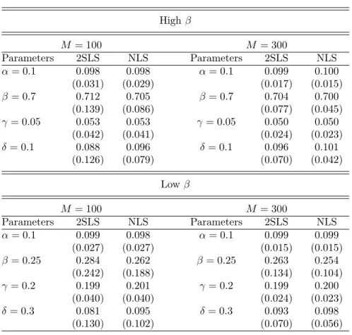
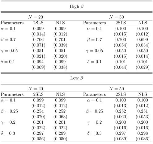
Results for two sets of parameters (high and low β), N = 30, M = 100 and 300—corresponding to N M = 3, 000 and 9, 000 observations—are presented in Table 1. Both estimators display moderate small-sample bias. Bias and estimates’ dispersion tend to be smaller for the NLS and when β is high. In the Appendix, we report results for the same parameters, N = 20 and 50, M = 500—corresponding to 10, 000 and 25, 000 observations—in Table5. Bias is then very low in all scenarios. Estimates’ dispersion is also low, and dispersion is lower for the NLS and at larger group sizes. Overall, these simulations show that the 2SLS and NLS estimators perform well in small samples of artificial data where binary outcomes are subject to endogenous peer effects. The NLS appears to outperform the 2SLS, especially when β is high.
Nonetheless, the 2SLS estimator has an important appealing feature for empirical applications: it can easily handle group fixed effects. Formally, suppose that α varies across groups r = 1, ..., M . We have
yr= αr1 + Xrθ + K
X
k=1
βkGk,ryr+ εr.
Since group size is bounded, the number of groups—and hence the number of parameters αr to estimate—
goes to infinity as the same rate as sample size. This is known as the incidental parameter problem and can notably yield inconsistent estimates of θ and β(K), seeLancaster(2000) for a review.
For linear models, however, a standard workaround is to rewrite the model in deviation from the group
23Assuming independence of the errors,Amemiya(1977) shows that weighted least squares is as efficient as the MLE. Moreover,
since the MLE is maximized using a numerical algorithm, one needs to ensure that all proposed parameters are such that Pi(θ) ∈ (0, 1). A similar issue arises for the implementation of the feasible weighted least squares: predicted probabilities used
average (seeCameron and Trivedi(2005), Section 21.6). Let Jr= Ir− 1r10r. We obtain Jryr= JrXrθ + K X k=1 βkJrGk,ryr+ Jrεr,
which does not depend on αr. The 2SLS strategy can then easily be adapted to estimate the model in
deviation.24 This issue may be critical in practice, in contexts where common unobservables may generate spurious correlations in outcomes.
Table 1: Monte Carlo Simulations – Number of Groups
High β M = 100 M = 300 Parameters 2SLS NLS Parameters 2SLS NLS α = 0.1 0.098 0.098 α = 0.1 0.099 0.100 (0.031) (0.029) (0.017) (0.015) β = 0.7 0.712 0.705 β = 0.7 0.704 0.700 (0.139) (0.086) (0.077) (0.045) γ = 0.05 0.053 0.053 γ = 0.05 0.050 0.050 (0.042) (0.041) (0.024) (0.023) δ = 0.1 0.088 0.096 δ = 0.1 0.096 0.101 (0.126) (0.079) (0.070) (0.042) Low β M = 100 M = 300 Parameters 2SLS NLS Parameters 2SLS NLS α = 0.1 0.099 0.098 α = 0.1 0.099 0.099 (0.027) (0.027) (0.015) (0.015) β = 0.25 0.284 0.262 β = 0.25 0.263 0.254 (0.242) (0.188) (0.134) (0.104) γ = 0.2 0.199 0.201 γ = 0.2 0.199 0.200 (0.040) (0.040) (0.024) (0.023) δ = 0.3 0.081 0.095 δ = 0.3 0.093 0.098 (0.130) (0.102) (0.070) (0.056)
Note: For each simulation, M networks are generated among the N = 30 individuals using iid Bernoulli trials with a probability p = 0.1. Thus, the expected number of links for each individual is 0.1(N − 1). Values represent the average (standard deviation) of the 1000 simulations.
5
Applications
We now apply the linear framework to real data. To highlight differences with existing approaches, we revisit two studies: Lee, Li, and Lin (2014) on peer effects in teenage smoking and Ciliberto and Tamer(2009) on
24Identification may of course be affected by the presence of fixed effects. Bramoullé, Djebbari, and Fortin (2009) derive
entry into airline markets. We reanalyze the same data as that of the original studies. These reanalyses show the usefulness of the linear model (1) and of our proposed estimators for analyzing interactions in binary outcomes. They illustrate the main advantages of the linear framework: ease of implementation, readily available overidentification tests, and the ability to handle fixed effects. In contrast, existing nonlinear approaches are generally computationally demanding, lack overidentification tests, and cannot handle large sets of fixed effects. These reanalyses also help assess the robustness of existing results.
We find similar qualitative results as those ofLee, Li, and Lin (2014). Furthermore, we find that these results are robust to the inclusion of school-grade fixed effects. By contrast, we find opposite qualitative results from those found by Ciliberto and Tamer (2009). While we cannot rule out that these differences are induced by the different assumptions, we observe that the econometric method proposed by Ciliberto and Tamer(2009) suffers from a severe curse of dimensionality. This curse does not affect estimations based on model (1). Moreover, overidentification tests are rejected in both applications, which suggests that these existing analyses suffer from problems of endogeneity.
5.1
Peer effects in teenage smoking
In this Section, we revisit the analysis of peer effects in teenage smoking of Lee, Li, and Lin(2014).25 This study is based on data from the National Longitudinal Survey of Adolescent to Adult Health, or Add Health, which provides rich information on the outcomes, behaviors, and characteristics of middle and high school students in the US. The data notably include detailed information on self-reported friendship relationships and has been widely used to analyze peer effects in networks. For the sake of comparison, we focus on the same sample, outcomes, characteristics, and networks as Lee, Li, and Lin(2014).
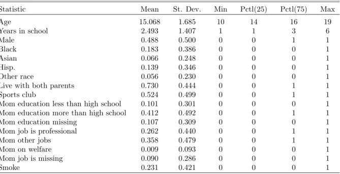
The data come from Wave I of the In-School Add Health survey, collected from 1994 to 1995. The sample contains information on the smoking behavior of 74,783 students in 127 schools. Lee, Li, and Lin (2014) classify a student as a non-smoker if they declared having never smoked or smoked only once or twice in the past twelve months. A student’s peers are his or her self-reported friends in the same school and grade. There are 532 school-grade groups, and hence the overall network is composed of 532 disjoint subnetworks. Summary statistics are presented in Table6 of Appendix7.1. The proportion of smokers among students is 23%.
To analyze peer effects on binary outcomes,Lee, Li, and Lin (2014) develop an incomplete information framework, extending Brock and Durlauf (2001) to networks. Their econometric framework can be micro-founded as follows, see also Liu (2019). Assume that agents have linear deterministic relative utilities (5) and preference shocks −ei. Assume further that the ei’s are independent and identically distributed with
a cumulative distribution function F . The expected relative utility of playing yi = 1 for agent i is equal
to E(ui(1, y−i) − ui(0, y−i)|ei, x) = fi(x, θ) − 12 + βPjgijE(yj|ei, x) − ei. Recall, Pi = P(yi = 1|x). By
independence, E(yj|ei, x) = E(yj|x) = Pj in a Bayes-Nash equilibrium. Therefore, Bayes-Nash equilibria are
characterized by the fixed-point equation Pi= F (fi− 1 2+ β X j gijPj), (9)
which corresponds to equation (1) inLee, Li, and Lin(2014).
By contrast, model (2) yields Pi = fi + βPjgijPj. Theorem 3 clarifies the conditions under which
model (2) can be viewed as a particular case of this framework: reduced-form errors must be uncorrelated, interactions must be moderate, and preference shocks must be uniformly distributed. Lee, Li, and Lin(2014) consider a logit framework in their empirical analysis. They assume that the probability that student i smokes tobacco is equal to
Pi=
exp(α + xiγ +Pjgijxjδ + βPjgijPj)
1 + exp(α + xiγ +Pjgijxjδ + βPjgijPj)
. (10)
They propose to estimate the model via an iterative simulated maximum likelihood. Each iteration has two steps: solving for Pi’s in the nonlinear fixed-point equation (10), conditional on parameter values, and
then re-estimating parameters through (simulated) maximum likelihood, conditional on these Pi’s. These
two steps are repeated until convergence. Their preferred specification includes contextual and endogenous peer effects, fixed effects at the school level, and random effects at the school-grade level. They find evidence of statistically significant, positive endogenous peer effects, with estimates of β ranging from 0.598 to 0.665. Their approach has two drawbacks. First, it is computationally demanding and involves a series of relatively high-dimensional nonlinear optimizations and fixed-point computations. This will likely limit the application of the method to other data and may make estimation unfeasible for larger data sets. Second, and as discussed by Lee, Li, and Lin(2014) in Section IV.B, the model cannot be estimated in deviations. This complicates the inclusion of group fixed effects, a main means of controlling for correlated effects. Simply including group dummies may be computationally unfeasible and may bias the estimates due to the incidental parameter problem.
In contrast, these drawbacks are absent from the 2SLS estimation of the linear model (2). Fixed effects can be eliminated by taking deviations from the group average. As well, efficient computation of 2SLS estimates are pre-programmed in standard statistical software and can be computed quickly even for massive data sets. We therefore reanalyze the same data assuming that model (2) holds.
Our estimation results are presented in Table 2. We consider specifications without fixed effects (NLS estimates in Column 1 and 2SLS estimates in Column 2), with school fixed effects (2SLS estimates in Column 3), and with school-grade fixed effects (2SLS estimates in Column 4). We see that estimates of the endogenous peer effects are remarkably similar to those obtained in Lee, Li, and Lin (2014): 0.568 in our preferred specification, compared to 0.666 in theirs. Standard errors have a similar magnitude, and this coefficient is very precisely estimated. Incorporating school-grade fixed effects only slightly decreases the estimate of the endogenous peer effect. The proportion of observations having a predicted probability between 0 and 1 lies
Table 2: Peer Effects on Smoking NLS 2SLS 2SLS 2SLS Endogenous effect 0.545 (0.038) 0.608 (0.062) 0.588 (0.058) 0.568 (0.058) Individual effects Constant -1.043 (0.089) -0.950 (0.141) - (-) - (-) Age 0.159 (0.012) 0.147 (0.020) 0.131 (0.018) 0.102 (0.027) Age2/10 -0.044 (0.004) -0.040 (0.007) -0.034 (0.006) -0.024 (0.009) Years in school 0.001 (0.002) 0.001 (0.002) -0.001 (0.002) 0.000 (0.002) Male 0.005 (0.004) 0.007 (0.005) 0.006 (0.005) 0.005 (0.005) Black -0.172 (0.006) -0.157 (0.007) -0.141 (0.007) -0.142 (0.007) Asian -0.080 (0.007) -0.070 (0.008) -0.056 (0.008) -0.059 (0.008) Hispanic -0.080 (0.006) -0.071 (0.009) -0.036 (0.007) -0.036 (0.007) Other race 0.029 (0.007) 0.022 (0.007) 0.028 (0.007) 0.027 (0.007) Live with both parents -0.046 (0.004) -0.039 (0.004) -0.042 (0.004) -0.042 (0.004) Sports club -0.040 (0.003) -0.036 (0.004) -0.039 (0.004) -0.040 (0.004) Mom education less than high school 0.010 (0.006) 0.007 (0.006) 0.010 (0.006) 0.009 (0.006) Mom education more than high school -0.012 (0.004) -0.008 (0.004) -0.007 (0.004) -0.007 (0.004) Mom education missing -0.030 (0.005) -0.026 (0.004) -0.021 (0.004) -0.021 (0.004) Mom job is professional 0.022 (0.004) 0.019 (0.005) 0.018 (0.005) 0.019 (0.005) Mom other jobs 0.024 (0.004) 0.021 (0.004) 0.021 (0.004) 0.021 (0.004) Mom on welfare 0.027 (0.017) 0.025 (0.016) 0.027 (0.016) 0.024 (0.016) Mom job is missing 0.014 (0.006) 0.008 (0.006) 0.009 (0.006) 0.009 (0.006) Contextual effects Age -0.007 (0.002) -0.010 (0.003) -0.009 (0.003) -0.010 (0.003) Age2/10 -0.002 (0.001) -0.001 (0.002) -0.001 (0.002) 0.000 (0.002) Years in school -0.003 (0.002) -0.003 (0.002) -0.005 (0.002) -0.004 (0.003) Male -0.006 (0.005) -0.015 (0.006) -0.018 (0.006) -0.017 (0.006) Black 0.062 (0.010) 0.065 (0.014) 0.062 (0.014) 0.059 (0.014) Asian 0.001 (0.010) 0.000 (0.012) 0.012 (0.013) 0.010 (0.013) Hispanic -0.010 (0.009) -0.004 (0.011) 0.026 (0.011) 0.024 (0.011) Other race 0.028 (0.011) 0.016 (0.013) 0.022 (0.014) 0.024 (0.014) Live with both parents -0.033 (0.007) -0.022 (0.009) -0.027 (0.008) -0.028 (0.008) Sports club -0.004 (0.005) -0.003 (0.007) -0.009 (0.007) -0.010 (0.007) Mom education less than high school 0.009 (0.009) 0.011 (0.011) 0.011 (0.011) 0.011 (0.011) Mom education more than high school -0.028 (0.006) -0.020 (0.008) -0.018 (0.008) -0.018 (0.008) Mom education missing 0.000 (0.009) 0.017 (0.011) 0.023 (0.011) 0.023 (0.011) Mom job is professional 0.011 (0.007) 0.001 (0.009) 0.003 (0.009) 0.004 (0.009) Mom other jobs 0.008 (0.006) -0.001 (0.007) 0.002 (0.008) 0.004 (0.008) Mom on welfare -0.025 (0.026) 0.005 (0.031) 0.015 (0.031) 0.010 (0.031) Mom job is missing 0.031 (0.010) 0.010 (0.011) 0.012 (0.011) 0.013 (0.011)
School fixed effects X
School-grade fixed effects X
Weak instruments 39.376 46.510 46.750
Sargan 44.449 57.190 60.431
Fraction predicted in [0, 1] 0.973 0.971 0.960
Note: Estimated coefficients and associated standard errors (in parenthesis). Estimation of linear model (2). Outcome is smoking. Summary statistics are presented in Table6of Appendix7.1. The number of observations is 74,783, the number of schools is 127, and the number of school-grades is 532. Standard errors are clustered at the grade-school level for the 2SLS estimators and are heteroscedastic-robust for the NLS estimator. Instruments for 2SLS estimations are generated using second-degree friends: G2X. The weak instrument tests are based on first-stage
F-tests. The test statistic under the null hypothesis that all instruments are weak follows a non-central χ2distribution (seeStock and Yogo(2005)).
The null hypothesis for all specifications is rejected at a confidence level < 1%. The null hypothesis of the Sargan test is that all instruments are exogenous. The test statistic follows a χ2distribution under the null hypothesis. The null hypothesis is rejected at < 1% for all specifications.
between 96% and 97%.26 Furthermore, in all specifications, the estimated coefficient satisfies the uniqueness condition of Theorem3.27
The characteristics of the students and their peers also affect smoking behavior. Another well-known advantage of a linear formulation is that the marginal impact of a characteristic on the outcome is simply equal to the characteristic’s estimated coefficient.28 For instance, being Black rather than White is associated with a 0.14 decrease in the likelihood to be a smoker. Students living with both parents and those with a high school–educated mother are less likely to smoke. Interestingly, these beneficial effects appear to spill over to students’ friends because a student having friends who live with both parents or with a high school–educated mother is also less likely to be a smoker.
Finally, we see that the joint validity of the instruments is rejected by overidentification tests. This is perhaps not surprising since there are 17 instruments here for one endogenous variable. Even though the instruments, jointly, appear to be strong, some instruments are likely to be weak. How best to estimate IV regressions and test overidentification in the presence of many weak instruments is an active area of research, see e.g.,Davidson and MacKinnon(2015),Carrasco and Tchuente(2016), andTchuente(2019).
5.2
Entry games and the airline industry
In this Section, we revisit the analysis of entry into airline markets ofCiliberto and Tamer(2009). As done in the previous Section, and for the sake of comparison, we analyze the same sample, variables, and data as
Ciliberto and Tamer(2009). The main data come from the 2001 Airline Origin and Destination Survey, a 10% sample of tickets collected by the US Department of Transportation. A market is defined as the trip between two airports, irrespective of intermediate transfer points and the direction of the flight. The sample includes 2,742 markets. Six firms are assumed to compete across all markets: American (AA), Delta (DL), United (UA), Southwest (WN), and two “composite” firms: Medium Airlines (MA) and Low-Cost Carriers (LCC). Each firm i is either present or absent from market m, yim∈ {0, 1}. The data include 10 variables assumed
to be exogenous: 8 market-level variables zm and 2 firm-market-level variables, xim: “airport presence” and
“cost”. We present summary statistics of these variables in Table7 of Appendix7.1.
Ciliberto and Tamer (2009) develop an econometric framework allowing for multiple equilibria. They consider static games of complete information based on variants of relative utility (5). The payoff for one firm of entering into a market depends linearly on the entry decisions of other firms. A key distinguishing assumption is that preference shocks are continuous and independent from observables in their framework.29 Equilibrium multiplicity can then generally not be avoided, and allowing for such multiplicity is central to their approach.
In their framework, a main object of interest is P(y|x, z), the probability of observing entry decisions
26Note that this proportion cannot be computed when the model is estimated in deviations. 27In linear-in-means model (2), this condition is equivalent to |β| < 1.
28InLee, Li, and Lin(2014), this corresponds to their “naive” estimation of the marginal effects. Our estimates and theirs
have similar signs, although their estimated marginal effects are generally larger in absolute value.