HAL Id: hal-00880716
https://hal.archives-ouvertes.fr/hal-00880716
Submitted on 7 Nov 2013
HAL is a multi-disciplinary open access
L’archive ouverte pluridisciplinaire HAL, est
Preventing premature convergence and proving the
optimality in evolutionary algorithms
Charlie Vanaret, Jean-Baptiste Gotteland, Nicolas Durand, Jean-Marc Alliot
To cite this version:
Charlie Vanaret, Jean-Baptiste Gotteland, Nicolas Durand, Jean-Marc Alliot. Preventing premature
convergence and proving the optimality in evolutionary algorithms. EA 2013, 11th International
Conference on Artificial Evolution, Oct 2013, Bordeaux, France. pp 84-94 ; ISBN : 9782953926736.
�hal-00880716�
Optimality in Evolutionary Algorithms
C. Vanaret1,2, J-B. Gotteland1,2, N. Durand1,2, and J-M. Alliot2
1
Ecole Nationale de l’Aviation Civile, Laboratoire de Math´ematiques Appliqu´ees, Informatique et Automatique pour l’A´erien, Toulouse, France
2
Institut de Recherche en Informatique de Toulouse, France {vanaret,gottelan,durand}@recherche.enac.fr
Abstract. Evolutionary Algorithms (EA) usually carry out an efficient explo-ration of the search-space, but get often trapped in local minima and do not prove the optimality of the solution. Interval-based techniques, on the other hand, yield a numerical proof of optimality of the solution. However, they may fail to con-verge within a reasonable time due to their inability to quickly compute a good approximation of the global minimum and their exponential complexity. The con-tribution of this paper is a hybrid algorithm called Charibde in which a partic-ular EA, Differential Evolution, cooperates with a Branch and Bound algorithm endowed with interval propagation techniques. It prevents premature convergence toward local optima and outperforms both deterministic and stochastic existing approaches. We demonstrate its efficiency on a benchmark of highly multimodal problems, for which we provide previously unknown global minima and certifi-cation of optimality.
1
Motivation
Evolutionary Algorithms (EA) have been widely used by the global optimization com-munity for their ability to handle complex problems with no assumption on continuity or differentiability. They generally converge toward satisfactory solutions, but may get trapped in local optima and provide suboptimal solutions. Moreover, their convergence remains hard to control due to their stochastic nature. On the other hand, exhaustive Branch and Bound methods based on Interval Analysis [1] guarantee rigorous bounds on the solutions to numerical optimization problems but are limited by their exponential complexity.
Few approaches attempted to hybridize EA and Branch and Bound algorithms in which lower bounds are computed using Interval Analysis. Integrative methods em-bed one algorithm within the other. Sotiropoulos et al. [2] used an Interval Branch and Bound (IB&B) to reduce the domain to a list of �-large subspaces. A Genetic Algo-rithm (GA) [3] was then initialized within each subspace to improve the upper bound of the global minimum. Zhang et al. [4] and Lei et al. [5] used respectively a GA and mind evolutionary computation within the IB&B to improve the bounds and the order of the list of remaining subspaces. In a previous communication [6], we proposed a cooperativeapproach combining the efficiency of a GA and the reliability of Interval
Analysis. We presented new optimality results for two multimodal benchmark func-tions (Michalewicz, dimension 12 and rotated Griewank, dimension 8), demonstrating the validity of the approach. However, techniques that exploit the analytical form of the objective function, such as local monotonicity and constraint programming, were not addressed. In this paper, we propose an advanced cooperative algorithm, Charibde (Cooperative Hybrid Algorithm using Reliable Interval-Based methods and Differential Evolution), in which a Differential Evolution algorithm cooperates with interval propa-gation methods. New optimal results achieved on a benchmark of difficult multimodal functions attest the substantial gain in performance.
The rest of the paper is organized as follows. Notations of Interval Analysis are introduced in Section 2 and interval-based techniques are presented in Section 3. The implementation of Charibde is detailed in Section 4. Results on a benchmark of test functions are given in Section 5.
2
Interval Analysis
Interval Analysis (IA) bounds round-off errors due to the use of floating-point arith-metic by computing interval operations with outward rounding [1]. Interval aritharith-metic extends real-valued functions to intervals.
Definition 1 (Notations).
– An interval X = [X, X] with floating-point bounds defines the set {x ∈ R | X ≤ x ≤ X}. IR denotes the set of real intervals. We note m(X) = 1
2(X + X) its midpoint
– A box X= (X1, . . . , Xn) is an interval vector. We note m(X) = (m(X1), . . . , m(Xn)) its midpoint
– We note ��(X, Y ) the convex hull of two boxes X and Y , that is the smallest box that contains X and Y
In the following, capital letters represent interval quantities (interval X) and bold let-ters represent vectors (box X, vector x).
Definition 2 (Interval extension; Natural interval extension). Let f : Rn→ R be a real-valued function. F : IRn→ IR is an interval extension of f if
∀X ∈ IRn, f(X) = {f (x) | x ∈ X} ⊂ F (X) ∀(X, Y) ∈ IRn, X ⊂ Y ⇒ F(X) ⊂ F (Y)
The natural interval extension FNis obtained by replacing the variables with their domains and real elementary operations with interval arithmetic operations.
The dependency problem The quality of enclosure of f(X) depends on the syntactic form of f : the natural interval extensions of different but equivalent expressions may yield different ranges (Example 1). In particular, IA generally computes a large over-estimation of the image due to multiple occurrences of a same variable, considered as
different variables. This ”dependency” problem is the main source of overestimation when using interval computations. However, appropriate rewriting of the expression may reduce or overcome dependency: if f is continuous inside a box, its natural inter-val extension FN yields the optimal image when each variable occurs only once in its expression.
Example 1. Let f(x) = x2−
2x, g(x) = x(x − 2) and h(x) = (x − 1)2−
1, where x ∈ X = [1, 4]. f , g and h have equivalent expressions, however computing their natural interval extensions yields
FN([1, 4]) = [1, 4] 2 −2 × [1, 4] = [1, 16] − [2, 8] = [−7, 14] GN([1, 4]) = [1, 4] × ([1, 4] − 2) = [1, 4] × [−1, 2] = [−4, 8] HN([1, 4]) = ([1, 4] − 1) 2 −1 = [0, 3]2−1 = [0, 9] − 1 = [−1, 8] We have f([1, 4]) = HN([1, 4]) ⊂ GN([1, 4]) ⊂ FN([1, 4]).
3
Interval-based techniques
Interval Branch and Bound algorithms (IB&B) exploit the conservative properties of interval extensions to rigorously bound global optima of numerical optimization problems [7]. The method consists in splitting the initial search-space into subspaces (branching) on which an interval extension F of the objective function f is evaluated (bounding). By keeping track of the best upper bound ˜f of the global minimum f∗
, boxes that certainly do not contain a global minimizer are discarded (Example 2). Re-maining boxes are stored to be processed at a later stage until the desired precision � is reached. The process is repeated until all boxes have been processed. Convergence cer-tifies that ˜f − f∗
< �, even in the presence of rounding errors. However, the exponential complexity of IB&B hinders the speed of convergence on large problems.
Example 2. Let us computemin
x∈Xf(x) = x 4−
4x2over the interval X
= [−1, 4]. The natural interval extension of f is FN(X) = X4−4X2. The floating-point evaluation f(1) = −3 yields an upper bound ˜f of f∗
. Evaluating FN on the subinterval[3, 4] reduces the overestimation induced by the dependency effect: FN([3, 4]) = [17, 220]. Since this enclosure is rigorous, ∀x ∈ [3, 4], f (x) ≥ 17 > ˜f = −3 ≥ f∗
. Therefore, the interval[3, 4] cannot contain a global minimizer and can be safely discarded.
Interval Constraint Programming (ICP) aims at solving systems of nonlinear equations and numerical optimization problems. Stemming from Interval Analysis and Interval Constraint Programming communities, filtering/contraction algorithms [8] nar-row the bounds of the variables without loss of solutions. The standard contraction algorithm HC4Revise [9] carries out a double exploration of the syntax tree of a con-straint to contract each occurrence of the variables (Example 3). It consists in an eval-uation (bottom-up) phase that computes the elementary operation of each node, and a backward (top-down) propagation phase using inverse functions.
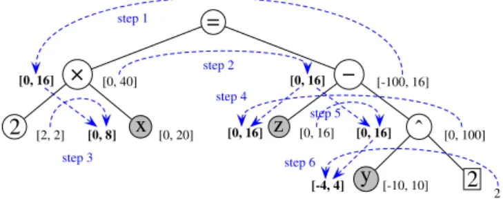
Example 3. Let2x = z − y2be an equality constraint, with x ∈[0, 20], y ∈ [−10, 10] and z ∈ [0, 16]. The elementary expressions are the nodes n1 = 2x, n2 = y2 and n3= z − n2.
The evaluation phase (Figure 1) computes n1 = 2 × [0, 20] = [0, 40], n2 = [−10, 10]2= [0, 100] and n 3= [0, 16] − [0, 100] = [−100, 16].
=
×
2
x
−
z
ˆ
y
2
2 [2, 2] [0, 20] [0, 40] [-10, 10] [0, 100] [0, 16] [-100, 16]Fig. 1. HC4Revise: evaluation phase
The propagation phase (Figure 2) starts by intersecting n1and n3(steps 1 and 2), then computes the inversion of each elementary expression (steps 3 to 6).
– steps 1 and 2: n� 1= n � 3= n1 ∩ n3= [0, 40] ∩ [−100, 16] = [0, 16] – step 3: x� = x ∩n�1 2 = [0, 20] ∩ [0, 8] = [0, 8] – step 4: z� = z ∩ (n2+ n�3) = [0, 16] ∩ ([0, 100] + [0, 16]) = [0, 16] – step 5: n� 2= n2∩(z�−n�3) = [0, 100] ∩ ([0, 16] − [0, 16]) = [0, 16] – step 6: y� = ��(y ∩ −�n� 2, y ∩�n � 2) = ��([−4, 0], [0, 4]) = [−4, 4]
=
×
2
x
−
z
ˆ
y
2
2 [2, 2] [0, 8] [0, 20] [0, 40] [0, 16] [-4, 4] [-10, 10] [-100, 16] [0, 16] [0, 100] [0, 16] [0, 16] [0, 16] step 3 step 1 step 2 step 4 step 5 step 6Fig. 2. HC4Revise: propagation phase
The initial box([0, 20], [−10, 10], [0, 16]) has been reduced to ([0, 8], [−4, 4], [0, 16]) without loss of solutions.
4
Charibde
algorithm
We consider the following global optimization problem and we assume that f is differ-entiable and that the analytical forms of f and its partial derivatives are available. We note n the dimension of the search-space.
min x∈D⊂Rn f(x)
subject to gi(x) ≤ 0, i ∈ {1, . . . , m}
Our original cooperative algorithm [6] combined a GA and an IB&B that ran inde-pendently, and cooperated by exchanging information through shared memory in order to accelerate the convergence. In this approach, the GA quickly finds satisfactory solu-tions that improve the upper bound ˜f of the global minimum, and allows the IB&B to prune parts of the search-space more efficiently.
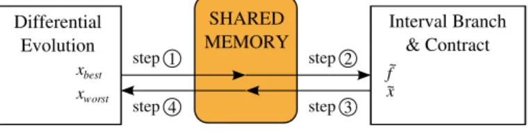
The current work extends the core method described in [6]. Its behavior is depicted in Figure 3. The interval-based algorithm embedded in Charibde follows a Branch & Contract (IB&C) scheme (described in Algorithm 1), namely an IB&B algorithm that integrates a contraction step based on HC4Revise. While an IB&B merely determines whether a box contains a global minimizer, an IB&C contracts the boxes with respect to the constraints gi(x) ≤ 0, i ∈ {1, . . . , m} (feasibility) or ∂x∂fi = 0, i ∈ {1, . . . , n}
(local optimality) and f ≤ ˜f . Exploiting the analytical form of the objective function and its derivatives achieves faster convergence of the hybrid algorithm, because efficient Constraint Programming techniques may prune parts of the search-space that cannot contain a global minimizer or that are infeasible. Filtering algorithms show particular efficiency when ˜f is a good approximation of the global minimum provided by the EA thread, hence the necessity to quickly find an incumbent solution. Charibde thus outperforms our previous algorithm by far.
Interval Branch & Contract SHARED MEMORY xworst xbest f~ x ~ step Differential Evolution 1 step 2 step 4 step 3
Fig. 3. Charibde algorithm
We notex the best known solution, such that F˜ (˜x) = ˜f . The cooperation between the two threads boils down to 4 main steps:
– step 1: Whenever the best known DE evaluation is improved, the best individual xbestis evaluated using IA. The upper bound of the image F(xbest) – guaranteed to be an upper bound of the global minimum – is stored in the shared memory – step 2: The best known upper bound F(xbest) is retrieved at each iteration from
is improved, it is updated to prune more efficiently parts of the search-space that cannot contain a (feasible) global minimizer
– step 3: Whenever the evaluation of the center m(X) of a box improves ˜f ,x and ˜˜ f are updated and stored in the shared memory in order to be integrated to the DE population
– step 4:x replaces the worst individual x˜ worst of DE, thus preventing premature convergence
In the following, we detail the implementations of the two main components of our algorithm: the deterministic IB&C thread and the stochastic DE thread.
4.1 Interval Branch & Contract thread
We noteL the priority queue in which the remaining boxes are stored and � the desired precision. The basic framework of IB&C algorithms is described in Algorithm 1.
Algorithm 1 Interval Branch and Contract framework
˜
f ←+∞ �best found upper bound
L ← {X0} �priority queue of boxes to process
repeat
Extract a box X from L �selection rule
Compute F(X) �bounding rule
if X cannot be eliminated then �cut-off test
Contract(X, ˜f) �filtering algorithms
Update ˜f �midpoint test
Bisect X into X1and X2 �branching rule
Store X1and X2inL
end if untilL = ∅ return( ˜f ,x)˜
The following rules have been experimentally tested and selected according to their performances:
Selection rule: The box X for which F(X) is the largest is extracted from L Bounding rule: Evaluating F(X) yields a rigorous enclosure of f (X)
Cut-off test: If ˜f − � < F(X), X is discarded as it cannot improve ˜f by more than � Midpoint test: If the evaluation of the midpoint of X improves ˜f , ˜f is updated Branching rule: X is bisected along the k-th dimension, where k is chosen
accord-ing to the round-robin method (one dimension after another). The two resultaccord-ing subboxes are inserted inL to be processed at a later stage
4.2 Differential Evolution thread
Differential Evolution (DE) is an EA that combines the coordinates of existing in-dividuals with a particular probability to generate new potential solutions [10]. It has
shown great potential for solving difficult optimization problems, and has few control parameters. Let us denote N P the population size, W > 0 the weighting factor and CR ∈ [0, 1] the crossover rate. For each individual x of the population, three other individuals u, v and w, all different and different from x, are randomly picked in the population. The newly generated individual y = (y1, . . . , yj, . . . , yn) is computed as follows: yj= � uj+ W × (vj−wj) if j= R or rand(0, 1) < CR xj otherwise (1)
R is a random index in{1, . . . , n} ensuring that at least one component of y differs from that of x. y replaces x in the population if f(y) < f (x).
Boundary constraints: When a component yjlies outside the bounds[Aj, Bj] of the search-space, the bounce-back method [11] replaces yjwith a component that lies between uj(the j-th component of u) and the admissible bound:
yj=
�
uj+ rand(0, 1)(Aj−uj), if yj< Aj
uj+ rand(0, 1)(Bj−uj), if yj> Bj (2)
Evaluation: Given inequality constraints {gi | i = 1, . . . , m}, the evaluation of an individual x is computed as a triplet (fx, nx, sx), where fxis the objective value, nxthe number of violated constraints and sx =
�m
i=1max(gi(x), 0). If at least one of the constraints is violated, the objective value is not computed
Selection: Given the evaluation triplets (fx, nx, sx) and (fy, ny, sy) of two candidate solutions x and y, the best individual to be kept for the next generation is computed as follows:
– if nx< nyor (nx = ny >0 and sx < sy) or (nx= ny = 0 and fx< fy) then x is kept
– otherwise, y replaces x
Termination: The DE has no termination criterion and stops only when the IB&C thread has reached convergence
5
Experimental results
Charibdehas been tested on the benchmark of functions reported in Table 1. This benchmark includes quadratic, polynomial and nonlinear functions, as well as bound-constrained and inequality-bound-constrained problems. Both the best known minimum in the literature and the certified global minimum3computed by Charibde are given. Some global minima may be analytically computed for separable or trivial functions, but for others (Rana and Egg Holder functions) no result concerning deterministic methods exists in the literature.
Partial derivatives of the objective function are computed using automatic differen-tiation [12]. To compute the partial derivatives of the functions that contain absolute values (Rana, Egg Holder, Schwefel and Keane), we use an interval extension based on the subderivative of| · | [13].
Table 1. Test functions with best known and certified minima
n Type Reference Best known Certified minimum
minimum by Charibde
Bound-Constrained Problems
Rana 4 nonlinear [14] - -1535.1243381
Egg Holder 10 nonlinear [15] -8247 [16] -8291.2400675249 Schwefel 10 nonlinear -4189.828873 [17] -4189.8288727 Rosenbrock 50 quadratic 0 0 Rastrigin 50 nonlinear 0 0 Michalewicz 75 nonlinear - -74.6218111876 Griewank 200 nonlinear 0 0 Inequality-Constrained Problems Tension 3 polynomial [18] 0.012665232788319 [19] 0.0126652328 Himmelblau 5 quadratic [18] -31025.560242 [20] -31025.5602424972 Welded Beam 4 nonlinear [18] 1.724852309 [21] 1.7248523085974 Keane 5 nonlinear [22] -0.634448687 [23] -0.6344486869
5.1 Computation of certified minima
The average results over 100 runs of Charibde are presented in Table 2. � is the numerical precision of the certified minimum such that ˜f − f∗
< �, (N P , W , CR) are the DE parameters, tmaxis the maximal computation time (in seconds), Smaxis the maximal size of the priority queueL, nefis the number of evaluations of the real-valued function f and neF = neDEF + neIB&CF is the number of evaluations of the interval function F computed in the DE thread (neDE
F ) and the IB&C thread (neIB&CF ). Note that neDE
F represents the number of improvements of the best DE evaluation. Because the DE thread keeps running as long as the IB&C thread has not achieved convergence, nefis generally much larger than the number of evaluations required to reach ˜f .
Table 2 shows that Charibde has achieved new optimality results for 3 func-tions (Rana, Egg Holder and Michalewicz) and has proven the optimality of the known minima of the other functions. As variables all have multiple occurrences in the expres-sion of Rana, Egg Holder and Keane’s functions, their natural interval extenexpres-sions are strongly subject to dependency. They are extremely difficult for interval-based solvers to optimize. Note that the constraints of Keane’s function do not contain variables with multiple occurrences, and are therefore not subject to dependency. However, they re-main highly combinatorial due to the sum and the product operations, which makes constraint propagation rather inefficient.
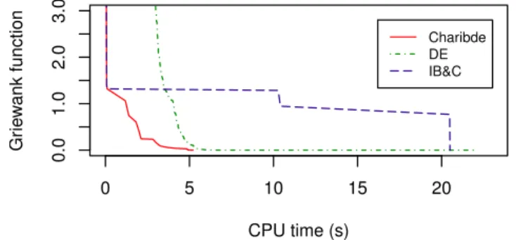
Figure 4 portrays the average comparison of performance between Charibde and standalone DE and IB&C over 100 runs on the Griewank function (n= 200). The stan-dalone DE remains stuck in a local optimum close to 0 after 22s, while the stanstan-dalone IB&C achieves convergence in 20.5s after several phases of stagnation. This is due to the (crude) upper bounds of f∗
evaluated at the center of the boxes. In Charibde, the IB&C provides the DE thread with a better solution than the current best known
evalua-Table 2. Average results over 100 runs n � N P W CR tmax Smax nef neF Bound-Constrained Problems Rana 4 10−6 50 0.7 0.5 222 42 274847000 47 + 27771415 Egg Holder 10 10−6 50 0.7 0.5 768 45 423230200 190 + 423230200 Schwefel 10 10−6 40 0.7 0.5 2.3 32 1462900 150 + 362290 Rosenbrock 50 10−12 40 0.7 0.9 3.3 531 368028 678 + 664914 Rastrigin 50 10−15 40 0.7 0 0.3 93 29372 29 + 42879 Michalewicz 75 10−9 70 0.5 0 138 187 6053495 1203 + 5796189 Griewank 200 10−12 50 0.5 0 11.8 134 188340 316 + 116624 Inequality-Constrained Problems Tension 3 10−9 50 0.7 0.9 3.8 80 1324026 113 + 1057964 Himmelblau 5 10−9 50 0.7 0.9 0.07 139 12147 104 + 36669 Beam 4 10−12 50 0.7 0.9 2.2 11 316966 166 + 54426 Keane 5 10−4 40 0.7 0.5 472 23 152402815 125 + 99273548
tion, which prevents premature convergence toward a local optimum. The convergence is eventually completed in 5.2s, with a numerical proof of optimality.
0 5 10 15 20 0.0 1.0 2.0 3.0 CPU time (s) Gr ie w ank function Charibde DE IB&C
Fig. 4. Comparison of Charibde and standalone DE and IB&C (Griewank function, n= 200)
5.2 A word on dependency
When partial derivatives are available, detecting local monotonicity with respect to a variable cancels the dependency effect due to this variable (Definition 3 and Example 4). In Definition 3, we call a monotonic variable a variable with respect to which f is monotonic.
Definition 3 (Monotonicity-based extension). Let f be a function involving the set of variablesV. Let X ⊆ V be a subset of k monotonic variables and W = V \ X the set
of variables not detected monotonic. If xiis an increasing (resp. decreasing) variable, we note x−
i = xiand x+i = xi (resp. x −
i = xi and x+i = xi). fminand fmaxare functions defined by:
fmin(W) = f (x − 1, . . . , x − k,W) fmax(W) = f (x+1, . . . , x + k,W) The monotonicity-based extension FMof f computes:
FM = [fmin(W), fmax(W)]
Example 4. Let f(x) = x2−2x and X = [1, 4]. As seen in Example 1, F
N([1, 4]) = [−7, 14]. The derivative of f is f�
(x) = 2x − 2, and F�
N([1, 4]) = 2 × [1, 4] − 2 = [0, 6] ≥ 0. f is thus increasing with respect to x ∈ X. Therefore, the monotonicity-based interval extension computes the optimal range: FM([1, 4]) = [F (X), F (X)] = [F (1), F (4)] = [−1, 8] = f ([1, 4]).
This powerful property has been exploited in [24] to enhance constraint propagation. However, the efficiency of this approach remains limited because the computation of partial derivatives is also subject to overestimation (Example 5).
Example 5. Let f(x) = x3−x2, f� (x) = 3x2−2x and x ∈ X = [0,2 3]. Since f� (X) = {f� (x) | x ∈ X} = [−1
3,0], f is decreasing with respect to x on X. However, F� (X) = 3 × [0,2 3] 2−2 × [0,2 3] = [− 4 3, 4
3] whose sign is not constant. Dependency precludes us from detecting the monotonicity of f . Bisecting X is necessary in order to reduce the overestimation of f�
(X) computed by IA.
6
Conclusion
Extending the basic concept of [6], we have presented in this paper a new cooperative hybrid algorithm, Charibde, in which a stochastic Differential Evolution algorithm (DE) cooperates with a deterministic Interval Branch and Contract algorithm (IB&C). The DE algorithm quickly finds incumbent solutions that help the IB&C to improve pruning the search-space using interval propagation techniques. Whenever the IB&C improves the best known upper bound ˜f of the global minimum f∗
, the corresponding solution is used as a new DE individual to avoid premature convergence toward local optima.
We have demonstrated the efficiency of this algorithm on a benchmark of diffi-cult multimodal functions. Previously unknown results have been presented for Rana, Egg Holder and Michalewicz functions, while other known minima have been certi-fied. By preventing premature convergence in the EA and providing the IB&C with a good approximation ˜f of f∗
, Charibde significantly outperforms its two standalone components.
References
2. Sotiropoulos, G.D., Stavropoulos, C.E., Vrahatis, N.M.: A new hybrid genetic algorithm for global optimization. In: Proceedings of second world congress on Nonlinear analysts, Elsevier Science Publishers Ltd. (1997) 4529–4538
3. Holland, J.H.: Adaptation in Natural and Artificial Systems. University of Michigan Press (1975)
4. Zhang, X., Liu, S.: A new interval-genetic algorithm. International Conference on Natural Computation 4 (2007) 193–197
5. Lei, Y., Chen, S.: A reliable parallel interval global optimization algorithm based on mind evolutionary computation. 2012 Seventh ChinaGrid Annual Conference (2009) 205–209 6. Alliot, J.M., Durand, N., Gianazza, D., Gotteland, J.B.: Finding and proving the optimum:
Cooperative stochastic and deterministic search. 20th European Conference on Artificial Intelligence (2012)
7. Hansen, E.: Global optimization using interval analysis. Dekker (1992)
8. Chabert, G., Jaulin, L.: Contractor programming. Artificial Intelligence 173 (2009) 1079– 1100
9. Benhamou, F., Goualard, F., Granvilliers, L., Puget, J.F.: Revising hull and box consistency. In: International Conference on Logic Programming, MIT press (1999) 230–244
10. Storn, R., Price, K.: Differential evolution - a simple and efficient heuristic for global opti-mization over continuous spaces. Journal of Global Optiopti-mization (1997) 341–359
11. Price, K., Storn, R., Lampinen, J.: Differential Evolution - A Practical Approach to Global Optimization. Natural Computing. Springer-Verlag (2006)
12. Rall, L.B.: Automatic differentiation: Techniques and applications. Lecture Notes in Com-puter Science (1981)
13. Kearfott, R.B.: Interval extensions of non-smooth functions for global optimization and nonlinear systems solvers. Computing 57 (1996) 57–149
14. Whitley, D., Mathias, K., Rana, S., Dzubera, J.: Evaluating evolutionary algorithms. Artifi-cial Intelligence 85 (1996) 245–276
15. Mishra, S.K.: Some new test functions for global optimization and performance of repulsive particle swarm method. Technical report, University Library of Munich, Germany (2006) 16. Sekaj, I.: Robust Parallel Genetic Algorithms with Re-initialisation. In: PPSN. (2004) 411–
419
17. Kim, Y.H., Lee, K.H., Yoon, Y.: Visualizing the search process of particle swarm optimiza-tion. In: Proceedings of the 11th Annual conference on Genetic and evolutionary computa-tion, ACM (2009) 49–56
18. Coello Coello, C.A.: Use of a self-adaptive penalty approach for engineering optimization problems. In: Computers in Industry. (1999) 113–127
19. Zhang, J., Zhou, Y., Deng, H.: Hybridizing particle swarm optimization with differential evolution based on feasibility rules. In: ICGIP 2012. Volume 8768. (2013)
20. Aguirre, A., Mu˜noz Zavala, A., Villa Diharce, E., Botello Rionda, S.: Copso: Constrained optimization via PSO algorithm. Technical report, CIMAT (2007)
21. Duenez-Guzman, E., Aguirre, A.: The baldwin effect as an optimization strategy. Technical report, CIMAT (2007)
22. Keane, A.J.: A brief comparison of some evolutionary optimization methods. In: Proceedings of the Conference on Applied Decision Technologies (Modern Heuristic Search Methods). Uxbrigde,1995, Wiley (1996) 255–272
23. Mishra, S.K.: Minimization of keane‘s bump function by the repulsive particle swarm and the differential evolution methods. Technical report, North-Eastern Hill University, Shillong (India) (2007)
24. Araya, I., Trombettoni, G., Neveu, B.: Exploiting monotonicity in interval constraint propa-gation. In: Proc. AAAI. (2010) 9–14