Transnational machine learning with screens for flagging bid-rigging cartels

WORKING

PAPERS

SES

N. 519

X.2020

Faculté des sciences économiques et sociales et du management

Transnational machine

learning with screens for

flagging bid-rigging cartels

Martin Huber,

David Imhof

and

Transnational machine learning with screens for flagging bid-rigging cartels

Martin Huber*, David Imhof** and Rieko Ishii*** * University of Fribourg, Dept. of Economics

** Corresponding Author, Swiss Competition Commission, University of Fribourg, Dept. of Economics, and Unidistance (Switzerland)

*** Shiga University, Dept. of Economics

Abstract: We investigate the transnational transferability of statistical screening methods originally developed using Swiss data for detecting bid-rigging cartels in Japan. We find that combining screens for the distribution of bids in tenders with machine learning to classify collusive vs. competitive tenders entails a correct classification rate of 88% to 93% when training and testing the method based on Japanese data from the so-called Okinawa bid-rigging cartel. As in Switzerland, bid rigging in Okinawa reduced the variance and increased the asymmetry in the distribution of bids. When pooling the data from both countries for training and testing the classification models, we still obtain correct classification rates of 82% to 88%. However, when training the models in data from one country to test their performance in the data from the other country, rates go down substantially, due to some screens for competitive Japanese tenders being similar to those for collusive Swiss tenders. Our results thus suggest that a country’s institutional context matters for the distribution of bids, such that a country-specific training of classification models is to be preferred over applying trained models across borders, even though some screens turn out to be more stable across countries than others.

Keywords: Bid rigging, screening methods, machine learning, random forest, ensemble methods. JEL classification: C21, C45, C52, D22, D40, K40, L40, L41.

Address for correspondence: David Imhof, Hallwylstrasse 4, 3003 Bern, Switzerland; [email protected]. Disclaimer: All views contained in this paper are solely those of the authors and cannot be attributed to the Swiss

1

Introduction

Bid rigging arises in many different markets related for instance to construction, highway mainte-nance, cement, timber, milk, rice, seafood procession or finance (see Feinstein et al., 1985; Porter and

Zona, 1993; Baldwin et al., 1997; Porter and Zona, 1999; Pesendorfer , 2000; Banerji and Meenakshi,

2004; Abrantes-Metz et al., 2006; Lee and Hahn, 2002; Bajari and Ye, 2003; Asker , 2010; Ishii, 2009;

Abrantes-Metz et al., 2012; Ishii, 2014; Hueschelrath and Veith, 2014; Bergman et al., 2019, among

others papers). It represents a significant share of cartel enforcement in many countries.1 The OECD estimates that the elimination of bid rigging could help reduce procurement prices by 20% or more.2 Since public procurement represents approximately 13% of the gross domestic product in OECD countries and 29% of government expenditure,3 the potential damage of bid rigging can be enor-mous. Unsurprisingly, the OECD recommends promoting pro-active methods for uncovering cartels (OECD, 2014). Responding to such need for pro-active statistical methods, Abrantes-Metz et al. (2006), Bolotova et al. (2008), Harrington (2007), Abrantes-Metz et al. (2012), Imhof et al. (2018),

Huber and Imhof (2019), Imhof (2019) and Chassang et al. (2020) have proposed different methods

for dismantling cartels based on descriptive statistics called screens. A legitimate question is whether one can successfully transfer such approaches that have been developed based on observations from one specific case or country to other institutional settings and countries to fight bid-rigging cartels on a transnational context.

In this study, we apply the screening methods suggested by Imhof et al. (2018), Huber and Imhof (2019), Imhof (2019) and Wallimann et al. (2020) in the context of bid rigging in Switzerland to the Okinawa bid-rigging cartel dismantled by the Japanese Fair Trade Commission (hereafter: JFTC) in June 2005. Since the identity of convicted bidders is known, one can categorize tenders as collusive when the respective bidders had participated in the tendering process before the opening of the JFTC’s investigation and as competitive after JFTC had sentenced the involved cartel participants. Our data cover three periods: the pre-inspection period including all tenders before the opening of the JFTC investigation in June 2005; the post-inspection period including all tenders between the opening of the JFTC investigation and the amendment of Japanese competition laws in January 2006; the post-amendment period including all tenders after the amendment of Japanese competition laws. The JFTC sentenced and sanctioned the involved cartel participants in the beginning of the post-amendment period in March 2006.

We show that combining statistical screens with machine learning is capable of dismantling the Okinawa bid-rigging cartel when using the Japanese data for training and testing the statistical models

1

See the OECD report Fighting Bid Rigging in Public Procurement, 2016, page 6, available at the following internet page: http://www.oecd.org/daf/competition/Fighting-bid-rigging-in-public-procurement-2016-implementation-report.pdf.

2_{See OECD internet page: http://www.oecd.org/competition/cartels/fightingbidrigginginpublicprocurement.htm.} 3

See the OECD report Fighting Bid Rigging in Public Procurement, 2016: http://www.oecd.org/daf/competition/Fighting-bid-rigging-in-public-procurement-2016-implementation-report.pdf.

for classifying collusive vs. competitive tenders. Qualitatively, bid rigging affects the distribution of bids in Japanese tenders in the same way as in Switzerland, by reducing the variance and increasing the asymmetry in bids. As machine learners, we consider the random forest, see Breiman (1996), and the “SuperLearner” ensemble method (including bagged regression tree, random forest, and neural network algorithms), see van der Laan et al. (2008). The overall correct classification rate varies between 88% and 93%, depending on the model (i.e. the number of predictors) and the machine learner considered. This suggests that our method can be an effective tool for promoting competition in public procurement in Japan.

In a next step, we merge the Japanese data with the Swiss data considered in Huber and Imhof (2019) to investigate the performance of our methods when being trained and tested in a transnational sample. We find correct classification rates between 82% and 88% and again, the variance screens turn out to be very good predictors. Finally, we use the data from one country for training the predictive models and those from the other country for testing model performance, which does considerably worse. Training in the Swiss data to test the trained models in the Okinawa data yields correct classification rates between 58% and 78%. Training in the Okinawa data and testing in the Swiss data performs even poorer with correct classification rates between 44% and 61%. This is worse than the screening method developed in Imhof et al. (2018), which relies on only two screens using a rule of thumb instead of machine learning and entails a correct classification rate of 72% in the Okinawa data. Apparently, a simple benchmarking approach can in some cases do better than trained models, if the training and testing data differ importantly.

Furthermore, the correct classification rate is unbalanced across collusive and competitive tenders when training in one country and testing in the other. This is especially the case when training in the Okinawa data to test in the Swiss data. In some cases, the machine learners are unable to predict the Swiss collusive tenders but predict with great accuracy the Swiss competitive tenders. This is due to some screens showing comparable values for collusive tenders in Switzerland and competitive tenders in Japan, which thus reduces the overall predictive performance of the trained model. A likely reason for this is that the Okinawa Prefecture Government (Hereafter: OPG) announces the reserve price or its cost estimate for a contract in the tendering process. Since bidders are disqualified if they bid above the reserve price, the distribution of bids in the tenders procured by the OPG is truncated, implying a lower variance of bids even under competition. Since such announcements do not exist in Switzerland, the distribution of bids is not truncated and has a higher variance. Our results thus suggest that a country’s institutions, e.g. the judicial and legislative environment as well as the procurement rules and procedures, implies that a predictive model trained in one country does not necessarily perform well when applied across borders in a different cultural context.

When dropping such variance screens with similar values in competitive Japanese and collusive Swiss bids and pre-selecting specific subsets of predictors, the correct classification rate improves to

approximately 70%, which is still considerably lower than under country-specific or pooled training and testing. Therefore, screens related to the asymmetry in the distribution of bids are to be preferred when using separate country data for training and testing. As bid rigging produces asymmetry in both Japan and Switzerland, screens capturing this asymmetry appear to be more robust to divergences in procurement rules than variance screens.

Finally and similar to Imhof et al. (2018), we perform an ex-ante or screening analysis using the Japanese data as it might be conducted by a competition agency in order to flag suspicious tenders. To this end, we use all episodes for which collusive and competitive tenders can be distinguished to train the machine-learning based models in order to predict bid rigging in the remaining Japanese data for which no information on the incidence of collusion is available. We then define a binary variable for the conspicuousness of contracts, taking the value of one if both the random forest and the ensemble method classify a tender as collusive. We indeed find many conspicuous contracts before the opening of the investigation of the JFTC and a decrease in the conspicuous contracts after JFTC sentenced the cartel participants. A regression analysis shows that conspicuousness is associated with higher contract prices, a reduced number of bidders, and specific geographic patterns. As in Ishii (2014), we also observe an association with specific rounding patterns in the bids, which is a result of the submission of phony or cover bids that lack a serious price calculation. All those findings corroborate the predictions of the machine learners and point to the potentially large gains of the application of machine learning with screens to promote competition in public procurement.

Our analysis contributes to a growing literature developing and implementing screening methods (see Abrantes-Metz et al., 2006; Harrington, 2007; Bolotova et al., 2008; Abrantes-Metz et al., 2012;

Jimenez and Perdiguero, 2012; OECD, 2014; Froeb et al., 2014). More specifically, it is related to

studies using screens for detecting bid-rigging cartels or analyzing the distribution of bids and the statistical patterns created in the distribution when bid rigging occurs (see Feinstein et al., 1985;

Imhof et al., 2018; Huber and Imhof , 2019; Imhof , 2019; Chassang et al., 2020; Wallimann et al.,

2020). Those papers contrast with papers which suggest and apply econometric tests for detecting bid-rigging cartels (see Porter and Zona, 1993; Baldwin et al., 1997; Porter and Zona, 1999; Pesendorfer , 2000; Bajari and Ye, 2003; Banerji and Meenakshi, 2004; Jakobsson, 2007; Aryal and Gabrielli, 2013;

Chotibhongs and Arditi, 2012a,b; Conley and Decarolis, 2016; Imhof , 2017; Bergman et al., 2019).

Such tests require data at the firm level, which are typically not readily available. Gathering such data might attract the attention of cartel participants, who might try to hide evidence prior to the opening of an investigation by a competition agency. Moreover, Imhof (2017) shows that econometric tests produce too many false negative results on the Ticino bid-rigging cartel, while screens perform considerably better. More broadly, our paper is also related to further studies discussing bid-rigging cartels or rings (see Baldwin et al., 1997; Porter and Zona, 1999; Banerji and Meenakshi, 2004; Lee

2016).

The remainder of the paper is organized as follows. Section 2 describes the Okinawa bid-rigging cartel and introduces the data. Section 3 discusses the statistical screens and machine learning algo-rithms, namely the random forest and an ensemble method. Section 4 applies the machine learners for training and testing predictive models for collusion in the Okinawa data. It also analyzes the per-formance when training models in the Japanese data and testing model perper-formance in the Swiss data and vice-versa, as well as when pooling data from both countries. Furthermore, it presents the results of a screening analysis when predicting bid rigging in parts of the Japanese data without information on the actual incidence of collusion. Section 5 concludes.

2

Bid-rigging and data

2.1 The Okinawa bid-rigging cartel and procurement

In our analysis, we consider procurement data from April 2003 to March 2007 obtained from the Okinawa Prefectural Government (hereafter: the OPG), that mainly contain tenders for civil engi-neering and building construction. In June 2005, the JFTC filed a bid-rigging investigation against a large number of firms involved in those tenders. The construction market in Okinawa exhibits several features facilitating collusion. First, the Okinawa Prefecture consists of 47 islands including Okinawa Main Island, which is the largest island with 1,200 km2. Such geographic conditions make it difficult to enter the market from outside of the prefecture. For the same reason, it is difficult to enter the market of one island from other islands. Hence, it appears inevitable that bidders repeatedly meet when they participate in the tenders.

Second, the OPG used an invitation procedure to procure construction works during the whole period. Under this procedure, the buyer chooses the companies allowed to submit a bid for a contract, which limits the entry to procurement tenders. Furthermore, the OPG announced the identity of the invited bidders prior to each tendering procedure until it changed its bidding system in January 2006. This enabled cartel participants to coordinate their bids and to detect whether an outsider of the bid-rigging cartel was invited in the tendering procedure. Third, the OPG systematically segmented the market and classified its contracts into five ranks from A+ and A to D with regard to the reserve price of each contract. The OPG also classified the bidders into five ranks according to the firm’s score of qualification.4 In the invitation procedure, the OPG selected bidders whose rank of qualification matches the rank of the contract. For instance, for a contract of rank A, the OPG invited bidders of rank A to submit a bid for that contract. However, bidders were often invited to submit bids for contracts with different ranks. For example, bidders with rank A+ were frequently invited to tenders

4

In Japan, firms intending to bid in public construction tenders are inspected and qualified according to different criteria, as for example the financial status or the experience in the construction field.

with rank A.

Two major events took place in the market during our data window. First, the JFTC launched an inspection on June 8, 2005 against firms participating in tenders for civil engineering and build-ing construction. In March 2006, the JFTC sanctioned 152 firms that were involved in bid-riggbuild-ing conspiracies. Penalties included fines and the suspension of bidding in public tenders for one to six months and most of the suspended firms were qualified as A+ contractors. 100 cartel participants rigged tenders in civil engineering, 103 participants tenders in building construction. The JFTC inves-tigation revealed that the bid-rigging cartel had started in April 2002 at the latest. Bid coordination took place in 94% and 98% of the civil engineering and construction building tenders, respectively, for contracts of rank A+ in the cartel period.

According to the JFTC, the process of bid coordination took the following form. Prior to each tender, the invited cartel participants met and those interested in the contract expressed their interest. If only one firm was interested, it would be the designated winner of the tender. Otherwise, the interested firms would engage in negotiations for determining the designated winner. During the negotiations, cartel participants considered factors such as the proximity of the contract location to each firm and the amount of each firm’s order backlog for allocating contracts among them. When they failed to reach an agreement, the designated winner was chosen by voting among bidders not interested in the contract. Cartel participants then agreed on the winning price and after that, each bidder other than the cartel winner independently calculated a phony bid that was higher than the bid of the designated cartel winner.

The second major event in our data window was the change of the Japanese competition law in January 2006. The Japanese Antimonopoly Act, amended and entering into force in January 2006, increased the fines by 50% and introduced a leniency program aiming at reducing the incentives to collude. Under the leniency program, penalties are reduced for companies providing specific and helpful information on collusion to the JFTC. Also the OPG changed its procurement system in January 2006, reacting to the bid-rigging cartel. First, the OPG increased the number of invited participants in each tendering procedure. For example, with such a change, the mode of invited bidders to contracts of rank A+ increased from 14 to 21. Second, the OPG also stopped announcing the identity of the invited bidders prior to bidding, which increased the difficulty of coordination among potential cartel participants. Under the new amended competition law and the new adapted procurement system, bid rigging became more difficult for potential cartel participants.

The procurement system of the OPG operates as follows. Whenever the OPG procures a con-struction contract, engineers estimate the costs of the concon-struction contract using an average firm as proxy. Based on this cost estimate, the OPG determines the reserve price for that contract, as well as its rank. The OPG then invites bidders to the tender with the same rank as the rank of the contract, which determines the number of invited bidders. The format of the tendering procedure follows a

first-price sealed-bid auction with a reserve price and a lowest acceptable price. The bidder with the lowest bid wins the contract only if its bid remains between the lowest acceptable price and the reserve price. The OPG rejects bids if they are below the lowest acceptable price, or above the reserve price.5 A further change in the procurement system concerned the reserve price, which was announced prior to each auction until January 2006, but was kept secret afterwards. However, this modification did most likely not importantly affect the bidding behavior, as after January 2006, the OPG instead announced its engineers’ cost estimate for each tender, which is typically slightly higher than the reserve price. In contrast, the lowest acceptable price was not revealed to the bidders at any point. It was set to 0.8 times the reserve price in 75% of the tenders until the change in the bidding system in 2006. After that change, the lowest acceptable price randomly oscillated in an interval between 0.8 and 0.85 times the reserve price.

We refer to the first period from April 2003 until the JFTC inspection starting in June 2005 as the “pre-inspection” period. The second period between the inspection and the amendment of the Antimonopoly Act in January 2006 is the “post-inspection” period. The final period after the amendment of the law is the “post-amendment” period, into which also fall the sentences by the JFTC in March 2006.

2.2 Data

The data are obtained from the OPG’s website. For each tender, the date of the tender, the name of the contract for which the auction is conducted, the type of construction (such as civil engineering), the project location, the winner, the winning price, the reserve price, the lowest acceptable price, the identity of each bidder and their bids are available for our analysis. During our data window, 17’798 invitations in 1’408 tenders were sent to bidders by the OPG, with 686 invitations being declined. 1’297 tenders concerned civil engineering and 111 building construction. We drop 74 bids in four tenders for civil engineering for which the reserve price is unavailable and therefore end up with 17’724 bids in 1’404 auctions. The data contain 645, 307, and 452 tenders for the pre-inspection, post-inspection and post-amendment periods, respectively.

In total, the OPG invited 1’767 firms to bid at least once in our data. Based on the JFTC’s documents, we identified 150 firms who received a bidding suspension due to being involved in bid rigging. We call these 150 firms “suspended bidders” or “cartel participants” and the other firms “un-suspended bidders”. Un“un-suspended bidders are, however, not necessarily competitive bidders, especially in the pre-inspection period.

For illustration, figure 1 shows the distribution of the ratio of the reserve price to the winning bid when only considering tenders with suspended bidders across periods. In the pre-inspection period,

5

In Japan, the lowest acceptable price is imposed in public procurement in order to disqualify a bid which is too low and is unlikely to reflect the true cost of the bidder.

Figure 1: The distribution of the ratio of the reserve price to the winning bid among suspended bidders

the ratio was between 0.95 and 1 in most tenders. In the post-inspection period, we find a greater dispersion of the ratio varying from 0.8 to 0.97. Such a bimodal distribution typically suggests that cartel participants rigged some contracts but competed on others. Therefore the post-inspection period appears to be a transition phase. In the post-inspection period, many winning bids were clustered at 0.8 of the reserve price, which corresponded to the lowest acceptable price prior to the change of the procurement system in January 2006, pointing to a competition among former cartel participant. We may presume that the 0.8 level for the lowest acceptable price seemed to be common knowledge even though it was officially a secret.

In the post-amendment period, when the lowest acceptable price was generally higher and less uniform after the change in the procurement system, the bids were clustered at 0.85. As the lowest acceptable price became less predictable in the post-amendment period, 10% of the bids were rejected for being too low, which was the case for less than 1% of the bids in the earlier two periods. The maximal financial harm caused by cartels in the pre-inspection period may be estimated by the difference between the winning bid and the lowest acceptable price of 0.8. For 48 contracts A+, this yields an average loss of 33’725’046 YEN with a total of 1’618’802’232 YEN.6

6

This corresponds to an average loss of approximately 320’000 US Dollars and a total of approximately 15 billion US Dollars based on an exchange rate as of September 2020.

3

Screening and machine learning

3.1 Screens as predictors

We subsequently discuss three types of screens for describing the distribution of bids in tenders: screens for the variance of bids, screens for the asymmetry of bids and one screen for the uniformity of bids (see Huber and Imhof , 2019; Imhof , 2019; Wallimann et al., 2020).

Concerning empirical evidence on variance screens, Feinstein et al. (1985) noticed for instance that the coefficient of variation, defined as the standard deviation divided by the arithmetic mean of all bids in a tender, was considerably lower under bid rigging when analysing highway construction contracts in North Carolina. Bolotova et al. (2008) observed a reduced variance of prices for a lysine cartel (but not for a citric acid cartel), while Abrantes-Metz et al. (2006) did so for frozen perch when a bid-rigging cartel was in place. Considering the coefficient of variation, Abrantes-Metz et al. (2012) provided evidence of manipulation in the daily bank quotes submitted to calculate the Dollar Libor. Jimenez and Perdiguero (2012) illustrated that markets with few competitors had a lower price variability and higher prices. In addition to our previous studies for Switzerland (see Imhof et al., 2018;

Huber and Imhof , 2019; Imhof , 2019; Wallimann et al., 2020), also other competition agencies have

found evidence for a reduced price variance in the case of collusion (see Esposito and Ferrero, 2006;

Ragazzo, 2012; Mena-Labarthe, 2012; Estrada and Vasquez, 2013). See also Athey et al. (2004) and Harrington and Chen (2006) for two theoretical (rather than empirical) contributions demonstrating

a decrease in the variance of prices when firms collude.

The reduction of the variance can be explained as follows. Under competition, the support of the distribution of bids is determined by the lowest and the highest bid in a tender. If a bid-rigging cartel wants to raise its profit, all cartel participants need to agree to bid higher than the lowest bid under competition, which changes the support of the distribution of bids. It implies a reduction of the variance if the increase above the lowest bid in a competitive situation is substantial (in order to realize profits) and if cartel members conjecture that the procurement agency can likely approximate the highest reasonable bid, e.g. based on experiences in previous tenders. In this case, the cartel cannot raise the bids of its participants beyond an unreasonably high value without risking to attract the attention of the procurement agency. The manipulated bids are then distributed on a reduced support, implying a decrease in the variance of bids. In the specific case of the OPG, the support of the distribution of bids expressed in terms of the ratio of the bids to the reserve price vary from 0.95 to 1 in the pre-inspection period and from 0.80 to 1 in the post-amendment period. We therefore expect the variance to be lower in the pre-inspection period compared to the variance in the post-amendment period.

Our first variance screen is the coefficient of variation (CV), a scale-invariant statistic considered for instance in Imhof et al. (2018), Huber and Imhof (2019) and Imhof (2019), which is formally

defined as follows: CVt= st ¯_b t , (1)

where sdt is the standard deviation and ¯bt the mean of the bids in some tender t. Another screen related to the support of the bids is the spread (SPD), which is calculated as follows:

SP Dt=

bmax,t− bmin,t

bmin,t

, (2)

where bmax,t denotes the maximum bid and bmin,t the minimum bid in some tender t (see Wallimann

et al., 2020).

In a bid-rigging cartel, participants not supposed to win the contract do not abstain from submit-ting bids for several reasons. First, a diminishing number of bidders could possibly raise suspicion, especially when the procurement agency invites firms to submit a bid for a contract as it was the case with the OPG. Second, it could be perceived as negative among the other participants not to cover a cartel fellow. Furthermore, the cost of a cover bid in terms of time and effort appears low as it need not be based on an accurate calculation, but must simply meet the requirement to be higher than the bid of the designated winner. Such a manipulation of bids may induce a convergence of coordinated bids, which we aim to capture by the kurtosis statistic (KURTO):

KU RT Ot= nt(nt+ 1) (n_t− 1)(n_t− 2)(n_t− 3) nt X i=1 (bit− ¯bt st )4− 3(nt− 1) 3 (n_t− 2)(n_t− 3), (3) where b_it denotes the bid i in tender t, n_t the number of bids in tender t, sd_t the standard deviation of bids, and ¯btthe mean of bids in that tender. As all tenders in our sample contain at least five bids, we are able to calculate the kurtosis for each tender.7

The coordination and manipulation of bids may also affect the symmetry of their distribution, which we aim to capture by specific screens also considered in Imhof et al. (2018), Huber and Imhof (2019), Imhof (2019) and Wallimann et al. (2020). These studies demonstrated that bid rigging increased the asymmetry in the distribution of bids in Swiss tenders. Such changes in the symmetry may be driven by differences between the two lowest bids in a tender or between losing bids, in line with theoretical findings by Marshall and Marx (2007) on manipulated bids in first-price auctions. Furthermore, Chassang et al. (2020) showed that a systematic appearance of substantial price gaps between the two lowest bids in tenders is at odds with competition and might imply bid-rigging conspiracies. At the same time, such gaps affect the symmetry of bids and related screens.

One screen targeting manipulations in the differences between the two lowest bids is the percentage difference (DIFFP):

DIF F Pt=

b2t− b1t b1t

, (4)

where b_1tis the lowest bid and b_2t the second lowest bid in some tender t. As an alternative difference measure, one may replace the denominator in (4) by the standard deviation of losing bids, which we refer to as relative distance (RD):

RDt=

b2t− b1t sdlosingbids,t

, (5)

where sdt,losingbids is the standard deviation calculated among the losing bids. Yet another normal-ization of the difference is based on using the mean difference between all adjacent bids in a tender as denominator, referred to as normalized distance (RDNOR):

RDN ORt= b2t− b1t (Pnt−1 i=1,j=i+1bjt−bit) nt−1 , (6)

where nt is the number of bids and bit, bjt are adjacent bids (in terms of price) in tender t, with bids being ordered increasingly. As a variation of (6), we exclude the lowest bid to use the mean difference between adjacent losing bids as denominator, referred to as alternative normalized distance (ALTRD):

RDALTt=

b2t− b1t (Pnt−1_i=2,j=i+1bjt−bit)

nt−2

, (7)

where b_1t is the lowest bid, b_2t the second lowest bid, n_t the number of bids and b_it, b_jt are adjacent losing bids in tender t, with bids being ordered increasingly. We also consider the simple (i.e. non-normalized) difference between the two lowest bids: D_t= b_2t− b_1t.

A further screen is the skewness statistic (SKEW) as a standard measure of symmetry in distri-butions: SKEWt= nt (nt− 1)(nt− 2) nt X i=1 (bit− ¯bt st )3, (8)

where nt denotes the number of the bids, bit the ith bid, sdt the standard deviation of the bids, and ¯_b

t the mean of the bids in tender t. Finally, we compute the nonparametric Kolmogorov-Smirnov statistic (KS) for measuring uniformity in the distribution of bids (see Wallimann et al., 2020). Even though competitive bids are not necessarily uniformly distributed, we suspect that coordination makes the distribution of bids even less uniform, which can be captured by a change in the following (KS) statistic: D+_t = max_i(x_it− it nt+ 1 ), D−_t = max_i( it nt+ 1 − x_it), KS_t= max(D+_t , D−_t ), (9)

where n_t is the number of bids in a tender, i_t the rank of a bid and x_it the standardized bid for the

ith rank in tender t. The standardized bids xit are the bids bit divided by the standard deviation of the bids in tender t for a normalized comparison of tenders with different contract values.

3.2 Models and machine learning

In our analysis based on machine learning, we investigate the performance of five models that differ in terms of the number of predictors and are referred to as model 1 to model 5. Model 1 includes all screens discussed in section 3.1 as well as two further characteristics as predictors, namely the number of bids and the contract value of a tender. Model 2 includes all screens, but no further characteristics like the number of bids or the contract value (which in contrast to the screens are scale-variant variables). Model 3 uses a subset of the screens, namely those related to the variance and the asymmetry of bids. Model 4 is based on the screens related to the variance and the uniformity of bids, model 5 on the screens related to the asymmetry and the uniformity of bids.

As in Huber and Imhof (2019), we apply a so-called ensemble method as machine learner, which is a weighted average of three algorithms: bagged regression trees, random forests and neural networks. In addition, we consider the performance of the random forests alone as a separate machine learner. For either method, we randomly divide the data into training and test samples, which contain 75% and 25% of the observations, respectively. Cross-validation in the training sample determines the optimal weight each of the three machine-learning algorithms obtains in the ensemble method. To this end we apply the “SuperLearner” package for “R” by van der Laan et al. (2008) with default values for bagged tree, random forest and neural network algorithms in the “ipred”, “partykit” and “nnet” packages, respectively, see Peters et al. (2002), Hothorn and Zeileis (2015) and Venables and

Ripley (2002).

Once the best model has been selected by finding the optimal weight for each machine learner in the training data, it is applied in the test sample to predict the outcomes and evaluate the out-of-sample performance by comparing the predicted to the actual outcomes. More concisely, we predict the collusion probability in the test sample and classify a tender as collusive whenever that probability is larger than or equal to 0.5 and as competitive otherwise. Our performance measure is the correct classification rate, which is the share of observations in the test data for which the classification based on our prediction matches the actually observed outcomes of collusion or competition. We repeat this procedure of randomly splitting the data into 75% training and 25% test data and evaluating the performance of the optimal model 100 times to calculate the average of the correct classification rate across the 100 data splits, which is our performance measure ultimately considered. For the random forests, the approach is analogous to that using the ensemble method, with the exception that cross-validation is not required in the training data as one need not weight alternative machine learners. As in Wallimann et al. (2020), the implementation is based on the “randomForest” package for “R” by

Breiman and Cutler (2018), using 1000 trees to estimate the predictive models in the training data.

Random forests and bagged trees as discussed in Breiman (1996), Ho (1995) and Breiman (2001) are so-called decision tree methods. Decision trees are obtained by recursively splitting the data

into subsamples in a way that minimizes the discrepancy between actual and predicted incidences of collusion or non-collusion within the subsamples according to some criterion like the Gini index. Both random forests and bagged trees consist of estimating such trees in a large number of samples repeatedly drawn from the original training data and averaging over the tree (or splitting) structures across samples to obtain predictions of collusion. However, one difference is that while bagged trees consider all predictors as candidates for further data splitting at each step, random forests only use a random subset of the total of predictors to reduce the correlation of tree structures across samples and thus, the variance of the machine learner (related to overfitting in correlated samples).

Finally, neural networks as discussed in McCulloch and Pitts (1943) and Ripley (1996) are different in spirit. Rather than splitting the data into subsamples based on specific predictor values, they aim at fitting a system of nonlinear functions that flexibly models the association of the predictors with collusion. Specifically, the predictors are used as inputs for nonlinear (for instance logit) intermediate functions, so called hidden nodes, which are themselves associated with the outcome of interest. Depending on the model complexity, hidden nodes may predict the outcome either directly or through other hidden nodes, such that several layers of hidden nodes allow modelling interactions between the functions and thus, predictors. The number of hidden nodes and layers gauges the flexibility of the model, with more parameters reducing the bias but increasing the variance.

4

Empirical analysis

4.1 Outcome definition and descriptive statistics in the Japanese data

Since we have knowledge about the suspended (i.e. sentenced) bidders by the JFTC, we consider a tender as collusive if a suspended bidder participated in it in the pre-inspection period, which mainly concerned contracts of rank A+ and to a lesser extent of ranks A, B and C. Only very few suspended bidders submitted bids for contracts of rank D and for this reason, we exclude any contracts of rank D from our analysis. We consider a tender as competitive if at least one suspended bidder participated in it in the post-amendment period, thus assuming that the presence of suspended bidders prevents the formation of new cartels in the short run. Since the descriptive price analysis in section 2.2 suggests that the post-inspection period is a transition phase, we discard those tenders in order to avoid the risk of contaminating the sample by an inaccurate classification of competitive and collusive tenders. Tables 1 and 2 report descriptive statistics for all predictors in the competitive and collusive tenders. Table 3 provides the results of Mann-Whitney and Kolmogorov-Smirnov tests for statistical differences in the predictors across competitive and collusive tenders. Regarding the variance screens, we find substantial differences between both periods for the coefficient of variation (CV) and the spread (SPD). The mean and median of the coefficient of variation amount to 1.16 and 0.44, respectively, in the collusive tenders as well as to 4.59 and 5.09, respectively, in competitive tenders. Concerning the

Table 1: Descriptive statistics for predictors in collusive tenders

Mean Std Min Lower Q. Median Upper Q. Max Obs

NBRBID 11.37 1.83 5 10 10 13 16 246 VALUE 76.55 68.88 9.3 23.30 45.82 129.00 280.56 246 CV 1.16 2.35 0.10 0.33 0.44 0.60 11.24 246 KURTO 1.16 2.63 -2.25 -0.50 0.47 2.14 14 246 SKEW -0.65 0.97 -3.48 -1.18 -0.69 -0.19 3.74 246 D 0.96 3.82 0.001 0.10 0.17 0.5 35.36 246 RD 2.18 5.24 0.0001 0.73 1.21 2.09 70.63 245 RDNOR 3.21 1.91 0.001 1.82 3 4.33 10.4 246 RDALT 6.06 12.42 0.001 2 3.93 6 171.6 245 DIFFP 0.93 2.84 0.002 0.26 0.41 0.66 23.37 246 SPD 0.04 0.06 0.003 0.01 0.02 0.02 0.28 246 KS 243.46 143.46 9.37 167.44 227.39 300.85 1051.36 246

Note: “Mean”, “Std”, “Min”, “Lower Q.”, “Median”, “Upper Q.”, “Max”, and “N” denote the mean, standard deviation, minimum, lower quartile, median, upper quartile, maximum and number of observations, respectively. “NBRBID”, “VALUE”, “CV”, “KURTO”, “SKEW”, “D”, “RD”, “RDNOR”, “RDALT”, “DIFFP”, “SPD” and “KS” denote the number of bids in a tender, the contract value, the coefficient of variation, the kurtosis, the skewness, the absolute difference between the two lowest bids in a tender, the relative distance, the normalized distance, the alternative relative distance, the percentage difference, the spread and the Kolmogorov-Smirnov statistic, respectively.

spread, the respective statistics are 0.04 and 0.02, respectively, in the collusive tenders as well as 0.17 and 0.18, respectively, in competitive tenders. The statistical tests reject the null hypothesis of no difference between the periods for both the CV and the SPD as reported in table 3.

The differences are less substantial for the kurtosis statistic (KURTO), with a mean and median of 1.16 and 0.44, respectively, in the collusive periods as well as 1.69 and 0.19, respectively, in the competitive tenders. While the Mann-Whitney test does not reject the null hypothesis of no difference between both periods, the Kolmogorov-Smirnov test does so at any conventional level of significance. The rejection is mostly driven by a higher standard deviation of the kurtosis statistic in the competitive tenders of 4.02 compared to 2.6 in the collusive tenders. With regard to the Kolmogorov-Smirnov statistic (KS), the mean and median strongly differ across collusive tenders (243.46 and 227.39) and competitive tenders (49.67 and 20.92), respectively and both statistical tests reject the null hypothesis. The distribution of bids is significantly less uniform in collusive than in competitive tenders.

Among the screens for the asymmetry of bids, we find important differences across periods w.r.t. the relative distance (RD), the normalized distance (RDNOR) and the alternative distance (ALTRD). For the relative distance, the mean and median amount to 2.18 and 1.21, respectively, in the collusive tenders, but to only 0.77 and 0.22 in the competitive tenders. Differences are similarly strong for the alternative and the normalized distance. Turning to the skewness statistic, the mean and median in the collusive tenders (-0.65 and -0.69) are substantially lower than in the competitive tenders (0.50 and 0.33). As reported in table 3, all statistical tests reject the null hypothesis. Also the differences in the

Table 2: Descriptive statistics for predictors in competitive tenders

Mean Std Min Lower Q. Median Upper Q. Max Obs

NBRBID 16.19 3.34 5 14 16 19 23 192 VALUE 83.90 68.50 9.99 26.66 59.70 133.48 244.85 192 CV 4.59 2.67 0.35 1.70 5.09 6.48 12.53 192 KURTO 1.69 4.02 -1.99 -1.04 0.19 2.96 19.65 192 SKEW 0.50 1.41 -2.46 -0.49 0.33 1.44 4.36 192 D 1.30 4.62 0.003 0.07 0.22 1.003 56.34 192 RD 0.77 2.60 0.0004 0.04 0.22 0.72 33.92 192 RDNOR 1.73 2.11 0.002 0.15 0.89 2.56 10.76 192 RDALT 2.62 5.08 0.002 0.14 0.87 2.88 48 192 DIFFP 2.06 5.62 0.002 0.17 0.52 1.51 53.54 192 SPD 0.17 0.12 0.01 0.06 0.18 0.23 1.11 192 KS 49.67 60.19 9.16 16.32 20.92 60.21 290.33 192

Note: “Mean”, “Std”, “Min”, “Lower Q.”, “Median”, “Upper Q.”, “Max”, and “N” denote the mean, standard deviation, minimum, lower quartile, median, upper quartile, maximum and number of observations, respectively. “NBRBID”, “VALUE”, “CV”, “KURTO”, “SKEW”, “D”, “RD”, “RDNOR”, “RDALT”, “DIFFP”, “SPD” and “KS” denote the number of bids in a tender, the contract value, the coefficient of variation, the kurtosis, the skewness, the absolute difference between the two lowest bids in a tender, the relative distance, the normalized distance, the alternative relative distance, the percentage difference, the spread and the Kolmogorov-Smirnov statistic, respectively.

non-normalized difference between the two lowest bids (D) are statistically significant across collusive and competitive periods, even though they are not that substantial in absolute terms. Concerning the percentage difference between the two lowest bids (DIFFP), the means (0.93 vs. 2.06) and standard deviations (2.84 vs. 5.62) are quite different across periods, while the medians are more similar (0.41 vs. 0.52). Also in this case, the statistical tests yield rather low p-values.

We consider two further tender-specific characteristics that are not among the scale-invariant screens outlined in section 3.1. The first is the number of bids in a tender (NUMBID), for which we again find significant differences, with the mean and median amounting to 11.37 and 10, respectively, in the collusive tenders and to 16.19 and 16, respectively, in the competitive tenders. This increase in bidders per tender during the competitive period was intended by the OPG’s decision to increase the number of invited bidders in the post-amendment period. The second characteristic is the contract value in million JPY (VALUE), whose mean and median are 76.55 and 45.82, respectively, among the collusive tenders, while the respective numbers are 83.90 and 59.69 among the competitive tenders. The statistical tests do not reject the null hypothesis in this case. All in all, however, we find substantial and very often statistically significant differences in the screens across collusive and competitive periods.

4.2 Training and testing in the Japanese data

Table 4 reports the results for the out-of-sample performance of our machine learners when training and testing in the Japanese data. Model 1 yields a correct classification rate of 93.7% and 92.2% for

Table 3: Statistical tests for the predictors between collusive and competitive tenders Screens z-statistic p-value MW KSstat p-value KS

NBRBIDS 14.66 < .0001 6.84 < .0001 VALUE 1.43 0.1530 1.13 0.1542 CV 13.94 < .0001 7.90 < .0001 KURTO -1.10 0.2734 1.64 0.0093 SKEW 9.16 < .0001 4.68 < .0001 D 1.56 0.1189 1.65 0.0084 RD -10.95 < .0001 5.64 < .0001 RDNOR -8.92 < .0001 4.68 < .0001 RDALT -9.20 < .0001 4.81 < .0001 DIFFP 1.95 0.0507 2.43 < .0001 SPD 14.27 < .0001 7.95 < .0001 KS -13.97 < .0001 7.90 < .0001

Note: “NBRBID”, “VALUE”, “CV”, “KURTO”, “SKEW”, “D”, “RD”, “RDNOR”, “RDALT”, “DIFFP”, “SPD” and “KS” denote the number of bids in a tender, the contract value, the coefficient of variation, the kurtosis, the skewness, the absolute difference between the two lowest bids in a tender, the relative distance, the normalized distance, the alternative relative distance, the percentage difference, the spread and the Kolmogorov-Smirnov statistic, respectively. “Screens”, “z-statistic”, “p-value MW” denote the screens tested, the z-statistic of the Mann-Whitney test and the p-value of the Mann-Whitney test, respectively. “KSstat” and “p-value KS” denote the Kolmogorov-Smirnov statistic and the p-value of the Kolmogorov-Smirnov test, respectively

the random forest and the ensemble method, respectively, which is the highest one among all models considered. Including the number of bids or the contract value as further predictors in addition to the screens increases the classification accuracy by three to five percentage points.

Models 2 to 5 entail a rather similar correct classification rate for the random forest of 88.9%, 89.4%, 88.9% and 88.7%, respectively. The same applies to the ensemble method, with rates of 88.6%, 89.4%, 88.2% and 89%, respectively, such that both machine learners have a very decent and similar predictive performance. Compared to the application of machine learning in Swiss cartel data by

Huber and Imhof (2019), the correct classification rate for the Okinawa bid-rigging cartel is four to six

percentage points higher. This suggests that the screens originally investigated in the Swiss context can also perform well in other countries with a different institutional setting like Japan.

However, the performance is not uniform across the subgroups of truly collusive and truly com-petitive tenders, see table 4, with differences in correct classification rates amounting to three to six percentage points. While the random forest yields a higher correct classification rate among compet-itive tenders (i.e. fewer false poscompet-itive classifications of competcompet-itive tenders as collusion), the ensemble method performs better among collusive tenders (with fewer false negative classifications of collusive tenders as competition). Since our sample contains more collusive tenders (246) than competitive ones (192), one might have suspected the machine learners to be slightly better in classifying collusive tenders due to this imbalance, as it is the case for the ensemble method, but not for the random forest.

Table 4: Correct classification rates for the Japanese data

Random Forest Ensemble Method

All Tenders Coll. Tenders Comp. Tenders All Tenders Coll. Tenders Comp. Tenders

Model 1 0.937 0.910 0.958 0.922 0.935 0.907

Model 2 0.889 0.853 0.919 0.886 0.898 0.871

Model 3 0.894 0.870 0.914 0.894 0.910 0.873

Model 4 0.889 0.862 0.911 0.882 0.901 0.860

Model 5 0.887 0.856 0.911 0.890 0.907 0.869

Note: “All Tenders”. “Coll. Tenders” and “Comp. Tenders” denote all tenders, the collusive tenders and the competitive tenders, respectively.

Using the random forest as machine learner, Table 5 reports the mean decrease in the Gini co-efficient (MDG) when dropping each of the four best predictors in the respective model. The MDG thus provides a ranking of the most important predictors within each model, but does not allow for a comparison between models since the MDG depends on the number of predictors included in each model. In models 1, 2 and 3, we observe that the SPD and the CV are the best predictors in the random forest. If available in the respective model, the number of bids and the KS follow in terms of predictive power. When excluding the number of bids as in model 2, the RD comes in fourth place, however, with a substantial drop in the MDG. When additionally excluding the KS in model 3, the RDNOR comes in fourth place behind the RD. However, both predictors (RDNOR and RD) entail a lower MDG than the SPD and the CV. The analysis of predictor importance in the random forest suggests that screens for the variance or uniformity of bids are most capable of distinguishing competitive and collusive tenders in the Okinawa bid-rigging cartel.

Table 5: Predictor importance for the Japanese data Model 1 Model 2 Model 3 Imp. MDG Imp. MDG Imp. MDG SPD 31.2 SPD 40.3 SPD 42.9

CV 28.9 CV 35.3 CV 41.4 NBRBIDS 28.2 KS 34.7 RD 19.5 KS 28 RD 13.4 RDNOR 13.3

Note: “Imp.” and “MDG” denote important predictors in the random forest and the mean decrease in Gini index when dropping them. “KS”, “CV”, “SPD”, “RD”, “RDNOR”, and “NBRBID” denote the Kolmogorov-Smirnov statistic, the coefficient of variation, the spread, the relative distance, the normalized distance and the number of bids in a tender, respectively.

In order to examine the robustness of the correct classification rate w.r.t. omitting important predictors, we drop the CV and the SPD, which are the best predictors in models 1, 2 and 3. As shown in table 6, the correct classification rate of model 1 decreases by 4.3 and 5.3 percentage points

when using the ensemble method and the random forest, respectively. Yet, model 1 attains a correct classification rate as high as that of models 2, 3, 4 and 5 when including all predictors such that its performance remains very decent. Furthermore, discarding the CV and the SPD barely affects the performance of model 2, such that the correct classification rates of models 1 and 2 are quite similar in table 6. In contrast, model 3 now entails a lower classification rate of 84.2% and of 83.6%, corresponding to a performance decreases of 5.2 to 5.8 percentage points when using the random forest and the ensemble method, respectively, due to the omission of the two most important predictors. Except for the KURTO, model 3 then exclusively relies on screens for the asymmetry of bids. This suggests that asymmetry-based screens perform somewhat worse than screens based on the variance or uniformity of bids for dismantling the Okinawa bid-rigging cartel.

Table 6: Correct classification rates for the Japanese data when dropping the two best predictors

Random Forest Ensemble Method

All Tenders Coll. Tenders Comp. Tenders All Tenders Coll. Tenders Comp. Tenders

Model 1 0.884 0.910 0.857 0.877 0.894 0.858

Model 2 0.880 0.897 0.860 0.893 0.900 0.884

Model 3 0.842 0.872 0.805 0.836 0.870 0.794

Note: “All Tenders”. “Coll. Tenders” and “Comp. Tenders” denote all tenders, the collusive tenders and the competitive tenders, respectively.

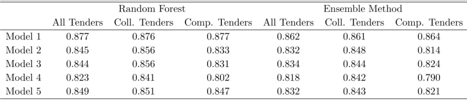
4.3 Training and testing in mixed or distinct country data

Table 7 reports the out-of-sample performance for the random forest and the ensemble method when training and testing in a merged data set containing observations from both Japan and Switzerland. We refer to Huber and Imhof (2019) for a detailed description of the Swiss data considered here, which consist of 584 tenders (299 collusive and 285 competitive tenders). The correct classification rates are lower than when training and testing in the Japanese data only (see table 4) for both the random forest and the ensemble method in all models, but still amount to a decent range of 81.8% to 87.7%. The correct classification rate of the random forest is roughly one percentage point higher than that of the ensemble method and both machine learners tend to perform better among collusive rather than competitive tenders. Table 8 provides the predictor importance in the merged data, with qualitatively similar results as in table 5 when only using the Japanese data. The CV, the SPD and the KS are the most predictive screens in the random forests of models 1, 2 and 3. Screens based on the variance and the uniformity of bids therefore have a higher predictive power than asymmetry-based screens.

We also consider the transnational transferability of trained models by using one country as training sample and the other as test sample. Table 9 reports the results when training the models in the Swiss data of Huber and Imhof (2019) and testing them in the Japanese data. For models 1 to 5,

Table 7: Correct classification rates when merging the Swiss and Japanese data

Random Forest Ensemble Method

All Tenders Coll. Tenders Comp. Tenders All Tenders Coll. Tenders Comp. Tenders

Model 1 0.877 0.876 0.877 0.862 0.861 0.864

Model 2 0.845 0.856 0.833 0.832 0.848 0.814

Model 3 0.844 0.856 0.831 0.834 0.844 0.824

Model 4 0.823 0.841 0.802 0.818 0.842 0.790

Model 5 0.849 0.851 0.847 0.832 0.843 0.821

Note: “All Tenders”. “Coll. Tenders” and “Comp. Tenders” denote all tenders, the collusive tenders and the competitive tenders, respectively.

Table 8: Predictor importance when merging the Swiss and Japanese data Model 1 Model 2 Model 3

Imp. MDG Imp. MDG Imp. MDG CV 60.5 SPREAD 73.1 SPD 80.9

SPD 60.7 CV 70.6 CV 79.4

KS 52.4 KS 56.7 RD 46.8

NBRBID 35.2 RD 36.6 RDNOR 45.1

Note: “Imp.” and “MDG” denote important predictors in the random forest and the mean decrease in Gini index when dropping them. “KS”, “CV”, “SPD”, “RD”, “RDNOR”, and “NBRBID” denote the Kolmogorov-Smirnov statistic, the coefficient of variation, the spread, the relative distance, the normalized distance and the number of bids in a tender, respectively.

the correct classification rates vary from 58.2% to 77.6%, which is substantially lower than before. Furthermore, the ensemble method clearly dominates, with correct classification rates that are 15.1 to 18.7 percentage points higher than those of the random forest. Concerning the different predictor sets, model 3 performs best overall, yielding the highest correct classification rate for the random forest (62.3%) and a close-to-best performance for the ensemble method (77.3%). However, we find substantial differences in terms of correct classification rates across subsamples of competitive and collusive tenders. The random forest does better in competitive than in collusive tenders. For the latter, the correct classification rates are only 40.5% to 47.6%, i.e. worse than random guessing by tossing a coin. The ensemble method performs better in collusive than in competitive tenders. For the latter, the correct classification rates are only 51% to 59.9%.

Overall, models that were trained in the Swiss data yield a quite unsatisfactory out-of-sample performance in the Japanese data. We therefore also investigate further models based on smaller sets of screens formed in ad hoc manner, in order to see whether this can improve classification accuracy despite relying on less predictors. As reported in Table 9, we find that the following subsets do comparably well: SKEW and RD, SKEW and RDALT, SKEW and KURTO, and SKEW and SPREAD. The last model yields the best performance with correct classification rates of 71.2% and 79.6% for the random forest and the ensemble method, respectively. All the comparably decently performing subsets include the SKEW as screen, which improves the predictive power of the random forest and entails in particular a better classification of collusive tenders than under models 1 to 5. Furthermore, the heterogeneity in the correct classification rates across collusive and competitive tenders is generally lower for both the random forest and the ensemble method when using those ad hoc models including only two screens. However, when adding one or more screens, the correct classification rates decrease and the heterogeneity across types of tenders again increase.

Table 9: Correct classification rates when training in the Swiss and testing in the Japanese data Random Forest Ensemble Method

All Tenders Coll. Tenders Comp. Tenders All Tenders Coll. Tenders Comp. Tenders

Model 1 0.589 0.474 0.693 0.776 0.914 0.559 Model 2 0.611 0.471 0.738 0.764 0.914 0.573 Model 3 0.622 0.471 0.762 0.773 0.914 0.594 Model 4 0.582 0.476 0.669 0.737 0.914 0.510 Model 5 0.597 0.405 0.789 0.776 0.914 0.599 SKEW, RD 0.621 0.625 0.625 0.707 0.844 0.600 SKEW, RDNOR 0.662 0.720 0.589 0.732 0.849 0.583 SKEW, RDALT 0.677 0.731 0.611 0.728 0.849 0.573 SKEW, DIFFP 0.492 0.177 0.843 0.654 0.547 0.792 SKEW, KS 0.544 0.467 0.601 0.732 0.914 0.500 SKEW, KURTO 0.636 0.633 0.646 0.686 0.698 0.672 SKEW, CV 0.676 0.785 0.537 0.73 0.914 0.495 SKEW, SPD 0.712 0.794 0.611 0.796 0.914 0.646

SKEW, RDNOR, RD, RDALT, KURTO 0.546 0.377 0.729 0.712 0.853 0.531

SKEW, RDNOR, RD, RDALT 0.579 0.569 0.569 0.719 0.861 0.536

SKEW, RDALT, KURTO 0.693 0.776 0.589 0.721 0.841 0.568

SKEW, RDNOR, KURTO 0.703 0.796 0.583 0.709 0.878 0.495

Note: “All Tenders”. “Coll. Tenders” and “Comp. Tenders” denote all tenders, the collusive tenders and the competitive tenders, respectively. “CV”, “KURTO”, “SKEW”, “D”, “RD”, “RDNOR”, “RDALT”, “DIFFP”, “SPD” and “KS” denote the coefficient of variation, the kurtosis, the skewness, the absolute difference between the two lowest bids in a tender, the relative distance, the normalized distance, the alternative relative distance, the percentage difference, the spread and the Kolmogorov-Smirnov statistic, respectively.

Furthermore, we apply the benchmark-based screening method suggested by Imhof et al. (2018) to the Japanese data, which comes without machine learning step for determining the best predictors (in the Swiss data), but instead relies on a rule of thumb based on only two screens, namely the CV and the RD. A shown in table 10, the method yields a correct classification rate of 72.1% overall, or of 60.4% for collusive tenders and 87% for competitive tenders. The approach of Imhof et al. (2018) thus performs as well as the best-trained models using the random forest and only in some cases, the ensemble method entails a higher correct classification rate.

Table 10: Results of Imhof et alii (2018) for the Japanese data Tenders Imhof et alii (2018)

All Tenders 0.721 Coll. Tenders 0.604 Comp. Tenders 0.870

Note: “All Tenders”. “Coll. Tenders” and “Comp. Tenders” denote all tenders, the collusive tenders and the competitive tenders, respectively.

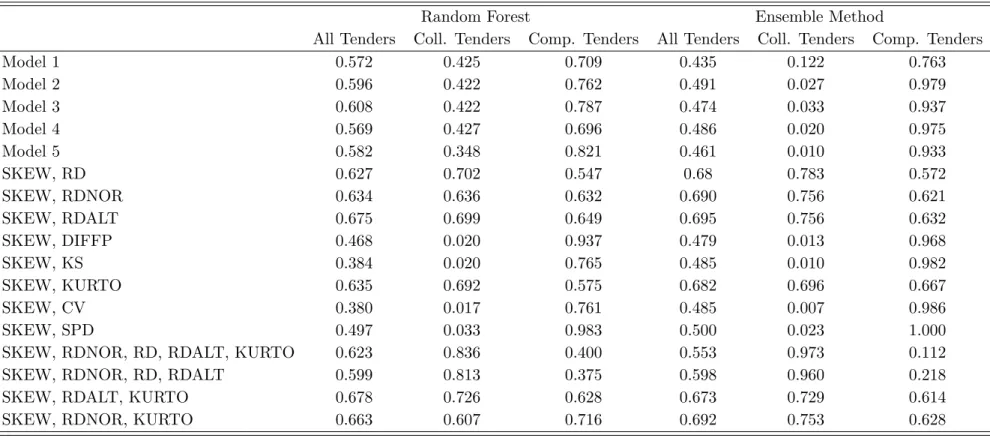
Also when training models in the Japanese data to test the out-of-sample performance in the Swiss data, we find the pattern that models with a restricted set of screens tend to work best, which goes against the aim of machine learning to identify the best predictors among a larger number of variables. As reported in table 11, models relying on SKEW and RD, SKEW and RDNOR, SKEW and RDALT as well as SKEW and KURTO yield correct classification rates of 62.7% to 69.5%. Using SKEW, RDALT and KURTO, the correct classifications amount to 67.8% and 67.3% for the random forest and the ensemble method, respectively, while for SKEW, RDNOR and KURTO, they are 66.3% and 69.2%, respectively. In contrast, models 1 to 5 perform even poorer when training in the Japanese data for testing in the Swiss data than vice versa. The ensemble method achieves overall correct classification rates below 50%, i.e. worse than tossing a coin. This is driven by the very low rates of at most 12.2% among collusive tenders, i.e. a massive failure to detect collusion. Even though the random forest does better than the ensemble method, its correct classification rates are far from being acceptable for models 1 to 5, too.

Table 11: Correct classification rates when training in the Japanese and testing in the Swiss data Random Forest Ensemble Method

All Tenders Coll. Tenders Comp. Tenders All Tenders Coll. Tenders Comp. Tenders

Model 1 0.572 0.425 0.709 0.435 0.122 0.763 Model 2 0.596 0.422 0.762 0.491 0.027 0.979 Model 3 0.608 0.422 0.787 0.474 0.033 0.937 Model 4 0.569 0.427 0.696 0.486 0.020 0.975 Model 5 0.582 0.348 0.821 0.461 0.010 0.933 SKEW, RD 0.627 0.702 0.547 0.68 0.783 0.572 SKEW, RDNOR 0.634 0.636 0.632 0.690 0.756 0.621 SKEW, RDALT 0.675 0.699 0.649 0.695 0.756 0.632 SKEW, DIFFP 0.468 0.020 0.937 0.479 0.013 0.968 SKEW, KS 0.384 0.020 0.765 0.485 0.010 0.982 SKEW, KURTO 0.635 0.692 0.575 0.682 0.696 0.667 SKEW, CV 0.380 0.017 0.761 0.485 0.007 0.986 SKEW, SPD 0.497 0.033 0.983 0.500 0.023 1.000

SKEW, RDNOR, RD, RDALT, KURTO 0.623 0.836 0.400 0.553 0.973 0.112

SKEW, RDNOR, RD, RDALT 0.599 0.813 0.375 0.598 0.960 0.218

SKEW, RDALT, KURTO 0.678 0.726 0.628 0.673 0.729 0.614

SKEW, RDNOR, KURTO 0.663 0.607 0.716 0.692 0.753 0.628

Note: “All Tenders”. “Coll. Tenders” and “Comp. Tenders” denote all tenders, the collusive tenders and the competitive tenders, respectively. “CV”, “KURTO”, “SKEW”, “D”, “RD”, “RDNOR”, “RDALT”, “DIFFP”, “SPD” and “KS” denote the coefficient of variation, the kurtosis, the skewness, the absolute difference between the two lowest bids in a tender, the relative distance, the normalized distance, the alternative relative distance, the percentage difference, the spread and the Kolmogorov-Smirnov statistic, respectively.

Figure 2: Density of the coefficient of variation by country and type of tenders

The poor performance can be explained by screens that have a relatively similar support and den-sity across collusive and competitive subsamples in different countries, see for instance the coefficient of variation (CV). While its mean and median in collusive tenders amount to 1.16 and 0.44 in Japan as well as 3.42 and 2.97 in Switzerland, the respective statistics under competition are 4.59 and 5.09 in Japan as well as 8.05 and 7.16 in Switzerland. Therefore, the CV in collusive Swiss tenders tends to be higher than in collusive Japanese tenders and more comparable to the competitive Japanese tenders, which creates issues for discriminating between collusion and competition across countries. As shown in figure 2, we observe a bi-modal distribution of the CV in the competitive tenders in Okinawa, while the peak of its density in the collusive Swiss tenders is located in-between. For this reason, if we train in the Okinawa data for testing in the Swiss data, a predictive method based on the CV recognizes almost all competitive Swiss tenders as competitive since their CVs are mostly either equal or above the CVs of the competitive Japanese tenders. However, it can barely recognize collusive tenders in Switzerland since their CVs fall into the range of competitive tenders in Okinawa. We find similar issues for the SPREAD, the KS and the DIFFPERC.

The ad hoc models presented in table 11 therefore perform better when excluding screens with common values across collusive and competitive periods in different countries and when including the SKEW, which has similar values within either competitive or collusive periods across countries. As shown in figure 3, it hold for both Japan and Switzerland that most of the density of the SKEW is concentrated between -2 and 0 in collusive tenders and between 0 and 3 in competitive tenders. Therefore, the SKEW is a good predictor when training in the Okinawa data to test out-of-sample prediction in the Swiss data (and vice versa). Further suitable screens are the RD, the RDNOR and the RDALT.

Figure 3: Density of the skewness by country and type of tenders

In conclusion, when merging the Swiss and the Japanese data, machine learning is able to correctly classify more than eight out of ten tenders. When training separately in one country for testing in the other, however, the performance of machine learning can drop to an unacceptably low level due to the mentioned support issues, while the rule of thumb-based screening method suggested by Imhof

et al. (2018) correctly classifies seven out of ten tenders. If one, however, selects specific subsets of

predictors, also machine learning can attain a correct classification rate of roughly seven out of ten. In our data, screens for the asymmetry of bids turn out to be most accurate for this exercise, as they seem to be quite robust to institutional differences in the tendering procedure across countries.

With the exception of KURTO, screens for the variance and the uniformity of bids turned out to be less suitable, as their values appear more context-specific and thus less transferable across countries. In our case, this issue is likely driven by the fact that in the Okinawa tendering procedure, bidders have information about the cost estimates of engineers or the reserve price set by the procurement agency, implying that cartel participants can rely on price information when rigging the tenders. Most of them bid just below the cost estimates or the reserve price when they collude, which truncates the distribution of bids and reduces its support as well as its variance. In contrast, in Switzerland bidders do not have access to cost estimates when trying to rig a contract such that the distribution of bids is not truncated. Unsurprisingly, the variance of collusive bids is therefore higher in Switzerland.

4.4 Ex-ante analysis: an example how to screen markets

In the previous analyses, we used information on collusive and competitive tenders for building models using random forests and the ensemble methods in the training data in order to evaluate their predictive performance in the test data, which obviously requires ex-post information about whether tenders were

collusive or competitive. In what follows, we perform a prediction in unseen data where the presence of absence or cartels is not clear, in order to see whether our method points to systematic collusion in that data. We therefore perform an ex-ante or screening analysis as in Imhof et al. (2018), just like a competition agency would do by applying a trained classification model to newly obtained data on tenders in order to assess the likelihood of cartel formation.

For training, we consider both the random forest and the ensemble method based on model 2, i.e. the specification using all screens, but not the scale-dependent characteristics NUMBID and VALUE. To maximize the sample size for training, we now use all the Japanese data with information on collusion and competition as training data, i.e. all observations either used in the training or test samples to obtain the results of section 4.2. We then apply the trained models to the remaining observations from Japan, i.e. all tenders of the post-inspection period as well as the pre-inspection and post-amendment periods without suspended bidders in the Okinawa data (and also including contracts of rank D), where the presence of collusion is ambiguous. Among these 950 tenders, we classify those as conspicuous (i.e. likely collusive) whose predicted probability of bid rigging is equal to or higher than 0.5 according to both the random forest and the ensemble method. Only 5% of the tenders are classified as collusive by one machine learner but not the other one, in which case a tender is classified as competitive. Therefore, the random forest and the ensemble method agree in 95% of the tenders.

Table 12 reports the contracts classified as conspicuous and competitive by type and period. For the pre-inspection period, 85% to 93% of the contracts of ranks A, B and C are classified as conspicuous. For contracts of rank D the share amounts to 61%, suggesting that this market segment was somewhat more competitive even before the opening of the JFTC’s investigation. In the post-inspection period, the share of tenders classified as competitive rises to 65% and 35% for contracts of ranks A+ and A, respectively, while it barely changes for the contracts of ranks C and D. Again, contracts of rank D have a higher share of competitively classified tenders than contracts of ranks B and C. In the post-amendment period, the majority of tenders is classified as competitive, even thought there is heterogeneity across contract types. 93%, 74% and 79% of the tenders among contracts of ranks A, B and D, respectively, are classified as competitive, but only 55% of those of rank C. This suggests that not all market participants have adapted their behavior after the change in the OGP procurement system following the amendment of Japanese competitive laws and the decision of the JFTC against the involved cartel participants. Among the bidders for contracts of rank C are apparently companies worth being scrutinized by an in-depth investigation concerning the possible incidence of bid rigging. Figure 4 shows the cumulative distribution of the normalized winning bid, i.e. the ratio of the winning price to the reserve price, separately for tenders classified as competitive and conspicuous. It reveals substantial differences across the groups of tenders. While 95% of the conspicuous tenders have a normalized winning bid between 0.95 and 1, the latter is lower among winning bids of tenders

Table 12: Tenders classified as conspicuous and competitive per contract type in the post-amendment period

Pre-inspection Post-inspection Pre-amendment Tenders Freq. Perc. Freq. Perc. Freq. Perc. Contract A+ Coll. 1 100% 6 35.3% 0 0% Comp. 0 0% 11 64.7% 6 100% All 1 17 6 Contract A Coll. 35 85.4% 43 65.2% 2 7.4% Comp. 6 14.6% 23 34.9% 25 92.6% All 41 66 27 Contract B Coll. 94 93.1% 63 84% 19 26% Comp. 7 6.9% 12 16% 54 74% All 101 75 73 Contract C Coll. 135 87.7% 79 85.9% 45 44.6% Comp. 19 12.3% 13 14.1% 56 55.4% All 154 92 101 Contract D Coll. 60 60.6% 24 60% 12 21.4% Comp. 39 39.4% 16 40% 44 78.6% All 99 40 56

Note: “All”. “Coll.” and “Comp.” denote all tenders, the collusive tenders and the competitive tenders, respectively.

classified as competitive and varies from 0.75 to 0.98.

In a further screening step, we analyze whether the conspicuousness of tenders as predicted by the machine learners is associated with several preselected characteristics (that partly overlap with the predictors used to train the models), which we deem informative for judging whether a group of tenders is potentially collusive or competitive. Dismantling such statistical associations may help detecting suspicious clusters in specific branches or geographic locations and thus contributes to validating our first step of the screening analysis. More concisely, we use the conspicuousness as dependent variable and estimate various logit specifications, in which different sets of characteristics enter as regressors. A first group of regressors reflects specific features of the tenders, namely the ratio of the winning bid to the reserve price (WINRES) to capture the price component of the winning bid, the number of bidders (NUMBID) and the contract value (VALUE) to approximate the size of the tendered project. A second group of regressors measures the roundness of bids in a tender. It includes the normalized number of zeros for the winning bid (WINROUND), i.e. the number of zeros in the winning bid divided by the number of digits in the winning bid. Similarly, we calculate the average of the normalized number of zeros for all bids in a tender (AVROUND) and the minimum normalized number of zeros (MINROUND). Ishii (2014) has shown that bid rigging may involve a higher incidence of rounded of bids, since collusive bidders do not calculate serious bids. Dummy variables for the contract type form the third group of regressors, dummies for procurement agencies the fourth. The fifth group includes a large set of geographic dummies for islands and municipalities. We progressively add the different