Combined dual emission laser induced fluorescence and particle image velocimetry to resolve temperature and velocity

Combined Dual Emission Laser Induced Fluorescence

and Particle Image Velocimetry

to Resolve Temperature and Velocity

by

Alan S. Grissino

B.S., Mechanical Engineering (1994)

Worcester Polytechnic Institute

Submitted to the Department of Mechanical Engineering in Partial Fulfillment of the Requirements for the Degree of

Master of Science in Mechanical Engineering

at the

Massachusetts Institute of Technology

February 2000

@2000 Massachusetts Institute of Technology

All rights reserved

Signature of Author

Department of Mechanical Engineering Jappary 14, 2000

Certified by

Douglas P. Hart Assistant rofessor of Mechanical Engineering

/ IThesis Supervisor

Accepted by

Ain A. Sonin Chairman, Department Committee on Graduate Students MASSACHUSETTS INSTITUTE

OF TECHNOLOGY

Combined Dual Emission Laser Induced Fluorescence

and Particle Image Velocimetry

to Resolve Temperature and Velocity

by

Alan S. Grissino

Submitted to the Department of Mechanical Engineering on January 14, 2000 in Partial Fulfillment of the Requirements for the Degree of Master of Science in

Mechanical Engineering

ABSTRACT

This thesis presents a novel technique for simultaneously measuring temperature and velocity. Using a high intensity ultrasonic field, small spherical tracer particles are formed and infused with two distinct fluorescent laser dyes. When protected by the particle encasement, dyes not normally soluble or otherwise compatible with the flow medium can be used. The fluorescence intensity of one dye is dependent upon temperature, the scalar quantity being measured, while the other temperature independent dye is used as a reference. By separating their emissions using narrow band optical filters, whole field temperature is measured simultaneously with flow velocity. Unlike other whole-field temperature measurement techniques, this combined PIT technique can be used with either gas or liquid, and is capable of resolving temperatures over an extended range. The use of DELIF tracer particles provides a high gain for superior PIV processing while enabling the use of LIF dyes.

Development of this technique is accomplished through the derivation of analysis techniques and algorithms. The effects of particle thermal response, particle size distribution, seeding density and laser light illumination are investigated using synthetically created images. To demonstrate the technique and utilize the theory and analysis methods a cold jet entering a hot tank of water is used to obtain real Particle Image Thermometry images.

Thesis Supervisor: Douglas P. Hart

Acknowledgements

There are many people whose support and guidance have made this research project possible. I would first like to thank my academic and thesis advisor, Professor Doug Hart, for his support, insight and approval. Doug's words of wisdom and seemingly endless supply of ideas helped to shape the body of this research and ensure that the correct issues were addressed. Through the ups and downs, we have persevered and seen this project through to a favorable end.

I would also like to thank those in the Fluid Mechanics Lab who aided in my struggle.

Without the help of Hugo, most of my image files would still be on a Mac! Carlos was an excellent sounding board for my ideas on PIV and particle fluorescence. Discussions with him helped to clear several issues, and his willingness to help out and let me use his experimental setup were invaluable. I also need to thank those in the Non-Newtonian Fluids Lab for not getting too mad at me when I blew up a batch of fluorescent particles.

I would like to thank TSI Incorporated of Minnesota, for the use of their resources and

time for experimentation. I thank Wing Lai for his help in coordinating the TSI/MIT effort, his help during experimentation and analysis of PIV images, and more importantly, his hospitality during my trips to the Land of 10,000 Lakes. Thanks to Dan Bjorkquist for his help with experimentation and his programming efforts which made my analysis easier.

Great thanks goes out to my GE Advanced Course in Engineering compatriots, Doug Walters, Garth Grover and Brent Brunell. From the early days of A-course through all of our classes and work leading up to this milestone, our combined support has helped to make this long road more enjoyable. Thanks also goes to my sponsor, GE Aircraft Engines, for their time (and money!). I would like to thank my wonderful family. The words of support and encouragement

from my parents and in-laws, especially Heinz and Peta, have been invaluable.

Most importantly, I would like to dedicate this thesis to my wife and children. Without the unyielding support and unearthly patience of my wife Liza, none of this would be possible. It has been a long, difficult road for all, and I cannot express enough how much I appreciate her support over the past four years. It has been a true testament to the strength of our marriage and family. I thank my two wonderful boys, Jason and Evan, whose patience with Daddy doing homework all the time was very much appreciated. I love you all very much, and now may

Table of Contents CHAPTER 1 - INTRODUCTION 11 1.1 PAST RESEARCH 11 1.2 GOALS 12 1.3 NOMENCLATURE 13 CHAPTER 2 - FLUORESCENCE 15 2.1 RATIOMETRIC TECHNIQUE 15

2.2 DYE SELECTION AND CHARACTERISTICS 17

2.3 SPECTRAL CONFLICTS AND IMAGE OVERLAP 17

2.4 DYE CONCENTRATION RATIO EFFECTS 18

CHAPTER 3 - PARTICLE MANUFACTURE 21

3.1 OVERVIEW 21

3.2 PARTICLE MANUFACTURING TECHNIQUE 21

3.3 RESULTS OF PARTICLE MANUFACTURE 24

CHAPTER 4 - PARTICLE THERMAL TIME RESPONSE 27

4.1 BACKGROUND 27

4.2 PHYSICAL SYSTEM MODEL 27

4.2.1 CONVECTION 29

4.2.2 CONDUCTION 34

4.2.3 RESULTS 41

4.2.4 DISCUSSION AND CONCLUSIONS 42

4.3 ONE TERM SERIES APPROXIMATION 44

4.3.1 SIZE DISTRIBUTION EFFECT ON TIME RESPONSE 45

5.1 5.1.1 5.1.2 5.1.3 5.2 5.2.1 5.2.2 5.3

INTENSITY AVERAGING TECHNIQUES

STRAIT MEAN TECHNIQUE

THRESHOLDING TECHNIQUE

EVALUATION OF AVERAGING TECHNIQUES

INTERROGATION WINDOW OPTIMIZATION WINDOW OVERLAP

WINDOW SIZE AND SEEDING DENSITY ANALYSIS TECHNIQUE CONCLUSIONS

49 50 50 56 60 60 63 68

CHAPTER 6 - EXPERIMENTAL PROOF-OF-CONCEPT 69

6.1 SETUP 69

6.2 EXPERIMENTAL PROCEDURE 71

6.3 RESULTS 72

CHAPTER 7 - CONCLUSIONS AND RECOMMENDATIONS 79

APPENDIX A - MATLABTm M-FILE SOURCE CODE FOR THERMAL SOLUTION

APPENDIX B -MATLABTm M-FILE SOURCE CODE FOR IMAGE ANALYSIS

APPENDIX C - DERIVATION OF VOLUME AVERAGED TEMPERATURE RESPONSE

REFERENCES

81

83

87

Table of Fiures

FIGURE 1 -RHODAMINE B ABSORPTION SPECTRUM VS. TEMPERATURE ... 16

FIGURE 2 -ILLUSTRATION OF SPECTRAL OVERLAP CONFLICT. Y-AXIS IS RELATIVE ABSORPTION/EMISSION IN ARBITRARY NO RM ALIZED UNITS... 18

FIGURE 3 -DYE CONCENTRATION RATIO EFFECTS... 20

FIGURE 4 -SPHERICAL TRACER PARTICLES WITH PIT DYES INFUSED. MAGNIFICATION IS APPROXIMATELY 1 OOX . 24 FIGURE 5 -REPRESENTATIVE PARTICLE SIZE DISTRIBUTION. BASED ON FIGURE 4. ... 25

FIGURE 6 - PARTICLE RELATIVE VELOCITY M OTION... 32

FIGURE 7 -PARTICLE THERMAL RESPONSE TIME. ... 42

FIGURE 8 -DISTRIBUTION EFFECT ON TIME RESPONSE ... 47

FIGURE 9 -TYPICAL 64 x 64 PIXEL REGION OF A PIT IMAGE... 51

FIGURE 10 - SAMPLE 64X64 PIXEL IMAGE FROM FIGURE 5 AFTER MEAN THRESHOLDIN.G ... 52

FIGURE 11 -PIXEL INTENSITY GRADIENT CONTOUR PLOT, FROM THE IMAGE IN FIGURE 9... 53

FIGURE 12 -SAMPLE IMAGE FROM FIGURE 5 AFTER GRADIENT THRESHOLDING ... 54

FIGURE 13 - REPRESENTATION OF GAUSSIAN PARTICLE PIXEL INTENSITY PROFILE ... 55

FIGURE 14(A) (TOP) SHOWS GAUSSIAN INTENSITY DISTRIBUTION ALONG SYMMETRY LINE. ... 55

FIGURE 15 -GAUSSIAN INTENSITY PROFILE AFTER GRADIENT CLIPPING... 56

FIGURE 16 -SYNTHETIC PIT IMAGE PAIR. LEFT IMAGE (A)... 57

FIGURE 17 - EXAMPLE PIT IMAGE ANALYSIS. X- AND Y- AXES ARE INDICES. RATIO CONTOUR LEGEND IS TO THE R IG H T ... 5 8 FIGURE 18 -EXAMPLE COMPARISON OF IMPOSED STEP DISTRIBUTION ALONG SYMMETRY PLANE (SOLID LINE) AND CALCULATED AVERAGE INTENSITY RATIO (CIRCLES) USING STRAIT MEAN ANALYSIS TECHNIQUE. ... 59

FIGURE 19 -EVALUATION OF INTERROGATION REGION AVERAGE INTENSITY METHODS... 60

FIGURE 20 -WINDOW OVERLAP STUDY. X-AXIS IS NORMALIZED DISTANCE ACROSS IMAGE. Y-AXIS IS DIFFERENCE BETWEEN CALCULATED AND ACTUAL VALUE ... 62

FIGURE 21 - WINDOW OVERLAP % VS. COMPUTATION TIME ... 63

FIGURE 22 - WINDOW SIZE EFFECTS, N=4000 ... ... 66

FIGURE 23 -W INDOW SIZE EFFECTS, N=2000 ... 67

FIGURE 24 -SCHEMATIC OF EXPERIMENTAL SETUP ... 69

FIGURE 25 -STEROSCOPIC CAMERA SCHEMATIC ILLUSTRATES THE SCHEIMPFLUG CRITERIA, WHERE OBJECT PLANE, IMAGE PLANE AND LENS PLANE ALL MEET AT A SINGLE POINT... 70

FIGURE 26 - TSI'S PIVCAMTM 10-30 STEREOSCOPIC PIV CAMERA SYSTEM ... 71

FIGURE 27 -PIT IMAGE OF COLD JET ENTERING HOT TANK, 580-NM FILTERED... 73

FIGURE 28 -PIT IMAGE OF COLD JET ENTERING HOT TANK, 630-NM FILTERED ... 75

Chapter 1 - Introduction

The field of experimental fluid mechanics has seen great advances in the qualitative measurement of whole field velocity through techniques such as Particle Image Velocimitry (PIV), Molecular Tagging Velocimetry (MTV), and Doppler Global Velocimitry (DGV). In many instances, however, temperature is as important, if not more so, than velocity (i.e., natural and forced convection, mixing, combustion, etc.). Several techniques for non-invasively measuring whole-field temperature have been developed, but none have taken hold and moved to the forefront as a viable and practical method for general use.

1.1 Past Research

As early as 1984, Ogden and Hendricks [1] and Rhee, Koseff and Street [2] used liquid crystals for a qualitative visualization of flow structures. Dabiri and Gharib [3] obtained quantitative temperature measurements with liquid crystals using computer analysis of recorded reflected light values. While their technique was very temperature sensitive,

(0.01 C), they reported results for only a narrow temperature range (30C). Nakajima, Utunomiya and Ikeda [4] obtained simultaneous measurement of velocity and temperature with separate systems. Laser Doppler Velocimetry (LDV) was used for velocity (standard Mie scattering exaggerated with 100 ptm polystyrene particles) and solute Rhodamine B (RhB) for temperature. The decrease of Rhodamine B's fluorescence intensity with temperature was used to calibrate and extract scalar temperature information.

Using a concept from the field of biology and biochemistry, Coppeta and Rogers [5] studied the measurement of scalar fluid quantities (temperature, concentration, pH) using a

ratiometric technique called Dual Emission Laser Induced Fluorescence (DELIF). Two

organic fluorescent dyes are used, one dependant on the scalar being measured and the other independent. They reported on the fluorescent characteristics of several dye combinations as potential for pH and temperature measurement. More recently, Sakakibara and Adrian [6] using Rhodamine B and Rhodamine 110 as the indicators utilized a ratiometric technique

By optically filtering the emitted light they calibrated the system and reported results over a

broad temperature range (20'C - 50'C).

1.2 Goals

Presented herein is a combined DELIF and PIV optical diagnostic technique, hereafter-called Particle Image Thermometry (PIT).

By embedding the dye indicators within the tracer particles used for PIV,

simultaneous measurement of velocity and temperature is achieved. Embedding the dyes within tracer particles provides a means of accurately controlling dye concentrations. Furthermore, dyes do not have to be chemically compatible with or soluble in the fluid medium. Consequently, measurements can be made in both gases and liquids with dye combinations not possible when soluble dyes are required. The ability to reuse the particles minimizes the financial impact if a costly dye must be used and the environmental impact if a hazardous dye must be used. The combination of these attributes greatly improves the practicality and accuracy of PIT as a means of temperature measurement as it enables the use

of a broad range of illumination sources, imaging methods, and dye combinations.

Paramount to the physical property benefits is the high gain signal that fluorescent particles provide for PIV. Indeed, the crux of this method is that the same particles used for PIV analysis are used for temperature analysis, negating the need for separate systems. The PIT data reduction and analysis can easily be incorporated into PIN software and analysis codes, providing true simultaneous calculations of velocity and temperature.

1.3 Nomenclature

General Notation

I Radiative intensity W

C Dye concentration mg/ml

V Volume m3

8 dye absorption coefficient m 2/gm

r radius m

d diameter m

k thermal conductivity W/m2 K

0 angle radians

Cp specific heat, constant pressure J/kgK Cv specific heat, constant volume J/kgK

p density kg/iM3

t time sec

T temperature 'C (or K)

O non-dimensionalized temperature

-h heat transfer coefficient W/m2K

R outer radius of sphere m

a thermal diffusivity m 2/sec

Pn n root of transcendental equation

-Cd drag coefficient

v velocity M/s

ge gravitational acceleration M/s2

M mass kg

As surface area m2

dynamic viscosity N-sec/m2

t* dimensionless time

MW molecular weight mol/gm

Subscripts

e exitation

f fluorescence (also fluid)

A camera A in dual-camera PIV setup B camera B in dual-camera PIV setup

abs absorption em emmision o final or external i initial Non-dimensionalized Parameters Re Reynolds number Pr Prandtl number Nu Nusselt number Bi Biot number

Chapter 2 - Fluorescence

2.1 Ratiometric Technique

Fluorescence is a radiative energy process categorized as a subset of the larger phosphorescent phenomenon. Certain chemical compounds react to incident energy stimulation by absorbing energy and transferring electrons within the molecule. These movements cause an increase in the electrical potential energy of the molecule, from a stable ground state to a higher order electronic state. When the molecule returns to the ground state, energy is released, usually in the form of light. The length of time that this emitted light persists is the basis for the general categorization of fluorophors. Fluorescence is typically defined when the time is less than about 10-8 seconds.

The intensity of fluorescence is dependent upon many factors, including intensity of incident excitation energy, dye concentration, volume, and characteristics of the dye. The general equation for intensity is

If = I, C V (1)

where I, is the intensity of the excitation beam at that point, C is the concentration of dye,

4

Coppetta and Rodgers investigations used separate dyes to minimize the variable effects of laser light intensity and other potential conflicts on detecting a scalar value of interest. This ratiometric technique uses one dye whose fluorescence is dependent on the scalar being measured (temperature, pH, etc.) and one dye, a reference dye, that is not. As reported by Coppetta et al., the ratioing concept is an established technique in the cellular biology field (Bassnett et al [7], Morris [8], and Parker et al. [9]).

This technique involves taking a ratio of the fluorescence intensity Equation (1) for each dye. We obtain,

I] ICA4T )A AV CAO(T)AE ₍₂

Equation (2) shows that the fluorescence ratio of the dyes is only a function of dye concentration, quantum efficiency, and absorption coefficient. The ratio has eliminated the laser sheet intensity. For the dye combination in the present investigation, the quantum efficiency (<) is the significant temperature dependent property. For the ratioing analysis to be accurate and viable, the incident laser intensity used to measure the fluorescence of the two dyes must be approximately equal. This is generally not possible with a single camera using a pulsed laser. However, it can be accomplished using a scanning Continuous Wave (CW) laser system with color wheel filter. It can also be done using a two-camera stereo PIV system with optical filters as in the current study. The fluorescence from both dyes is then recorded at the same time.

Recent studies of film thickness using LIF show that absorption of Rhodamine B may exhibit a temperature dependency. However, the author has only seen qualitative proof of this phenomenon, and the experiments performed are being done at high temperatures (200+ 'C). As seen in Figure 1, Coppetta and Rogers show that Rhodamine B absorption is essentially temperature independent for the temperature range of interest in this research (20-60'C).

1.00 10 0C -425"C --- 480C 0.75 - X 6n 0.50-0.25 0.00 -450 475 500 525 550 575 600 Wavelength (nm)

2.2 Dye Selection and Characteristics

The selection of a proper fluorescent dye combination for this technique is dependent on many experimental design considerations. These include the flow medium of interest, type of flow field, and others. The temperature dependent dye used in the present investigation is Rhodamine B known for it's strong dependence on temperature (about 2.3%/'K). Rhodamine B has been widely used in LIF studies due to its solubility characteristics and temperature dependence. With a peak absorption at around 556 nm, it is easily excited by either a frequency doubled Nd:YAG laser (532 nm) or the 514 nm line of an argon-ion laser. The peak emission of Rhodamine B occurs at approx. 580 nm.

The reference, temperature independent dye chosen is Pyrromethene 650 (PM650)

(1,2,3,5,6,7 - hexamethyl - 8 - cyanopyrromethene - difluoroborate complex, or BF₂ -complex). Pyrromethene 650 has a peak absorption around 588 nm (in Ethanol) and a peak emission at 625 nm. Although it's thermal stability is exceptional, it is not soluble in water. Table 1 shows properties for various dyes.

Table 1 -Dye Characteristics

Dye MW Xabs Xem

#

- mol/g nm nm - m2/g

PM650 301.15 588 624 0.54 0.0183

RhB 479.02 556 580 0.31 4.4

Rhl10 366.80 496 520 0.80 34

2.3 Spectral Conflicts and Image Overlap

Copetta and Rogers discuss three spectral type conflicts when using two fluorescent dyes. Their Type II conflict occurs when there is an overlap in the absorption band of one dye with the emission band of the other. Figure 2 illustrates an example of this type of interaction. This conflict results in the measured fluorescence of dye 1 being less than the actual emission, due to it being absorbed by dye 2 as it travels through the medium. However, for a constant path length, a calibration curve that is independent of path length can be constructed

by dividing the fluorescence ratios at all temperatures by the ratio at some arbitrary reference

value.

Such a Type II conflict exists when Rhodamine B and Pyrromethene 650 are used in combination. Despite this conflict (which can be overcome), PM650 was selected partially to illustrate the utility of a non-compatible (soluble) dye.

Emission Band Dye 1

Absorption Band

,,,ooDye 2

Wavelength (nm)

Figure 2 - Illustration of Spectral Overlap Conflict Y-axis is relative absorption/emission in arbitrary normalized units.

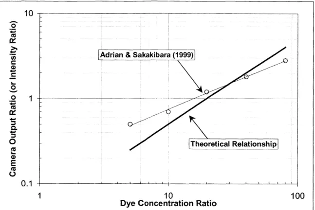
2.4 Dye Concentration Ratio Effects

Equation (2) shows that the intensity ratio is a function not only of temperature (through the quantum efficiency ratio), but also of the ratio of dye concentrations. In its simplest form this relationship is linear. Adrian & Sakakibara [6] accounted for imperfect separation of the two dye intensities, IA and 1B. Overlapping emission bands of the two dyes may cause some fraction of the light IA t0 be detected by camera B, and likewise, a fraction of light IB detected by camera A. Equation (2) can be reformulated to address this issue, as done

by Adrian et. al. The equation they arrive at takes this imperfect light filtering into account,

Ve CA/B C BA CAB C =3

(3)

SCA/BC AV C +A B CA =0

Experimental results for the two dyes used in their procedure (Rhodamine B and Rhodamine 110) are shown in Figure 3 by the curve-fit line and open symbols. Their evaluation of Equation (3) very closely matches the experimental results shown here. The solid line in the figure represents Equation (2) evaluated using the physical properties for RhB and Rhi 10 found in Table 1. As noted, this is a linear relationship. The experimental results (and prediction from Equation (3)) show the introduction of a nonlinear power relationship in the form Y = aXb. Adrian et. al., reason that an optimum value of Va/VP is

obtained when the signal-to-noise (S/N) ratio of each camera is the same. This is because the measurement of V"/VP can not have a S/N ratio higher than that of the lower S/N ratio a single camera, A or B. Put another way, the S/N ratio of Va/VP is maximized when the S/N ratio of V" and VP are equal. Since the camera gain (sensitivity) of each camera was set to the

same, this criteria is met when V"/VP = 1.

The measured data in Figure 3 shows that this occurs at a concentration ratio CA/CB Of

approximately 20. This agrees very well with the theoretical linear calculation, which also crosses 1.0 at exactly CA/CB of 20.

Figure 3 - Dye Concentration Ratio Effects 10

Adrian & Sakakibara (1999)

0

.2 1T

o Theoretical Relationship

0.1

1 10 100

Chapter 3 - Particle Manufacture

3.1 Overview

A key aspect technique presented here is the infusion of two separate fluorescent dyes

into the spherical tracer particles used for PIV. As reported by Frigerio [10], tracer particles for use in PIV applications must "...meet to very specific size, shape, density, and fluorescence requirements." There are very few commercial manufacturers of fluorescent tracer particles for such applications, and those that do exist charge as much as $250 per gram. This cost barrier prompted Frigerio and Hart to develop a manufacturing process for particles using their own internal equipment and labor resources. The trials of this initial effort are provided in Frigerio's thesis. The result of their efforts was particles made from a polyester monomer resin, linked with an external catalyst. The fluorescent dye was embedded in the particles during their creation. The approach is based on the fact that the surface tension properties of the resin causes spherical beads to be formed when placed into water. Frigerio's technique was utilized and modified for use in manufacturing PIT fluorescent tracer particles.

3.2 Particle Manufacturing Technique

The particle making procedure was resurrected for this research project, and successful batches of Rhodamine G (RhG) particles were made. However, creation of particles with two different fluorescent dyes proved to be more challenging. The fact that Pyrromethene 650 (PM650) is not water-soluble apparently adversely affected the resin curing process. Investigation revealed that the PM650 did not appear to be staying in solution with the resin at all. Many attempts were made using different concentrations of catalyst, dyes, and anti-emulsifying agents. Limited success was realized when the PM650 was first mixed with methanol, a substance in which it is soluble. This approach produced a usable batch for the current research, and the manufacturing process is reported here. It is noted that even at the time of this printing, research is ongoing in the Fluid Mechanics Laboratory at MIT to perfect the process of dual dye tracer particle manufacture.

Particles used here are manufactured from a catalyzed polyester and styrene monomer resin. Using the cavitation effects from a high intensity ultrasonic generator, the large spheres formed by the resin in the water solution are "hammered" apart. In combination with a magnetic stir bar, the power level and duration of the ultrasonic device (sonicator) are varied to produce desired particle size distributions. Through further sifting and sieving after the curing process is complete, controlled distributions with sizes ranging from less than 10 ptm up to 100 pm (and larger) in diameter are created.

The following procedure outlines the ingredients and steps used to create the dual dye particles used for the current research.

1. Ingredients:

0.7 gm Sodium Chloride, NaCl

0.2 gm Ammonium Thyocianate

0.5 gm Polyvinyl Alcohol (PVA) 5 mg Pyrromethene 650 (PM650) 100 mg Rhodamine B

Distilled water

25 ml methanol

100 ml polyester casting resin

Casting resin catalyst (methyl-ethyl-ketone-peroxide, MEKP)

2. Pour the 25 ml of methanol into a 50 ml or larger glass beaker. Add the 5 mg of

PM650 dye. Mix well.

3. Pour the 100 ml of casting resin into a 150 ml or greater glass beaker. Add the

PM650/methanol mixture and stir very well. Let the mixture stand until the methanol has evaporated from the mixture (about 1 hour).

4. While the resin mixture is evaporating, pour 400 ml of distilled water into a 500 or 600 ml glass beaker.

5. Place the beaker of water on a combination hot plate/magnetic stirrer. Begin to

6. Measure and add the Sodium Chloride, Ammonium Thiocynate and Polyvinyl

Alcohol to the water. While still mixing, heat to approx. 500C.

7. When the resin mixture has returned to the original 100 ml level (i.e., all of the

methanol has evaporated off), proceed to next step.

8. Transfer the resin mixture into a 500 or 600 ml glass beaker. Add 20+ drops of

catalyst (MEKP) to resin mixture and stir vigorously for 30 sec., taking care to scrape the sides and ensure extremely well combination.

NOTE: addition of the catalyst will begin the chemical reaction to bind the

polymer chains in the resin. It will start to become stiff very rapidly, so this step and the following must be performed quickly.

9. Place the resin beaker on the hot plate and very quickly pour in the water solution,

stirring vigorously. With the mag. stirrer operating, quickly place the sonicator horn into the mixture.

10. Run the sonicator on HI continuous power setting for 2 min 30 sec.

11. Heat the mixture to 70*C while mixing with stir bar. Turn off or remove from heat

and allow to cool back down to 30-50'C.

12. Repeat step 11 twice.

13. With heat off, stir for approx. 10 hours while particles are curing. (The heating

and cooling cycles of steps 11 and 12 speed up the chemical reaction).

The particles are cured now ready to be separated.

Using appropriate fine mesh metal sieves, filter and separate the particles to the desired sizes. Once sieved, add denatured alcohol to the particles and place back on stir-pad. Let stir in the alcohol for 10 hours. The particles should now be fully cured and bleached of any excess dye.

3.3 Results of Particle Manufacture

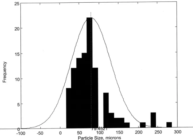
The above recipe and procedure results in remarkably spherical tracer particles, suitable for both normal PIV processes and the current PIT process. Figure 4 shows typical particles. The magnification is approximately 1 OOX.

Figure 4 -Spherical tracer particles with PIT dyes infused Magnification is approximately JOOX

Figure 5 illustrates the type of size distribution represented by the particles in Figure

25 20 L 15L-10 5 I I -100 -50 0 50 100 150

Particle Size, microns

200 250

Figure 5 - Representative Particle Size Distribution. Based on Figure 4.

U-300 0 I

U

Chapter 4 - Particle Thermal Time Response

4.1 Background

The PIT technique is reliant upon several assumptions about the physical system involved. Past experiments have utilized fluorescent dyes in aqueous solution. In solution, the dye molecules are an integral part of the water, and as such, will respond to changes in temperature in a time span on the same order of magnitude as the water. Therefore, the fluorescence.at a point in the water at any given time truly is an indicator of the temperature of the water at that point.

In the technique presented here, the dye is embedded in small spherical particles made of plastic. While the particles are very small (10-100 pm), they are still orders of magnitude larger than the surrounding water molecules. The particle will therefore have a finite thermal lag. Knowledge of this time lag, or thermal response time, is necessary when determining the size, scope, accuracy and materials for a given experiment. If the time response is much larger (order of magnitude) than either the presumed temperature and velocity time scale of the flow field or of the image capturing system, the results could be erroneous. The particles fluorescence indicates it's temperature at that instant in time, so if the particle has not reached nearly the same temperature as the surrounding fluid, then it will not represent the temperature of the fluid.

Having established that the particles exhibit a finite, perhaps relatively large thermal response time, it is the goal of the following chapter to provide both mathematical and physical meaning to the solution(s) of this problem.

4.2 Physical System Model

The problem presented here is one of a spherical particle immersed in a fluid (water in this case). As demonstrated in the previous section and shown in Figure 4, the spherical

assumption is valid. The next step is determining what boundary conditions are imposed on the spherical particles. This is a crucial step, as it governs both the mathematical solution and the physical interpretation of the resulting thermal time response.

For the given system of plastic particles in water, only conduction and convection will be considered as potential dominant modes of heat transfer. Described herein are several potential modeling situations which may (or may not) be viable representations of the particles. Subsequently, assumptions are applied and the mathematical formulation of each solution is derived and solved. Results are presented and argument is made for the most probable approach that models the real physical system.

All of the following analyses are based on the heat conduction equation for a sphere.

Combining Fouriers Law of Conduction with a control volume energy balance leads to the complete heat conduction equation (expressed in spherical coordinates). This is

1

a

kr +k si0 -2 (kT )+q = pc . (4)

r 2 ar j r r2 sin O /

rs

With the assumption that the heat flow is one dimensional (radial) and that the fluid properties are constant in both time and space, Equation (4) is reduced to

aT I k

_r

T(5)

at

r

r

&r

This equation is subject to an initial condition (temporal) and a boundary condition (spatial) at the surface. Temperature is a function of both time t and radius r. Solution of the differential equation varies by type of boundary conditions applied, but methods are prescribed in Carslaw and Jeager [11] and Schnieder [12].

4.2.1 Convection

4.2.1.1 Background

When posed with a situation of a solid material in contact with a fluid, as presented here, it is usually assumed that a convection boundary condition is present. The interaction of the fluid boundary layer and the solid surface at the contact interface dictates the mode of energy transport. Whether the movements of the shear layer at the interface is controlled by free or forced movement of the fluid far field, a heat transfer coefficient (h) inevitably enters the picture. The transient thermal solution of the sphere in such an environment is thus dictated by not only the environment temperature, but also by this heat transfer coefficient. This h along with the physical properties of the solid and fluid govern the flow of energy to and from the particle (and the fluid).

For the present system, it is arguable that there is a convection environment surrounding the particle. One major assumption in PIV analysis is that the particles do not disrupt the flow, and being close to neutrally buoyant, follow the fluid. Using the particles for thermometry, only fluid in the immediate vicinity of the particle is considered since the particle's fluorescence is meant to indicate the fluids temperature at that point in space. By combining these assumptions, it can be said that the particle has no relative motion with respect to the fluid, at least in close proximity to the particle. Convection heat transfer is by definition entirely dependent upon this relative motion. Therefore, it can be argued that convection is not the appropriate model for this system.

4.2.1.2 Physical and Mathematical Analysis

Despite the argument presented above, the convection solution is presented for comparison. Here, Ti is a known temperature at time t=O. The convection boundary condition

aT

-k = h, (T -T) at r = ro. (6)

ar

This condition states that the conductive heat flux at the surface is equal to the convective heat flux away from the surface. Here, T is the surface temperature of the sphere and To is the environment temperature in the surrounding fluid. As outlined in Schnieder et. al., the solution of this equation takes form through a Fourier Series analysis. The solution is

T(r, t)-- T _ 4(sin

p,-IpncosP.)

O(r, t)=--- e -smi, (7)

T -T1 2f3 -sin(2p,) jr, R

n = I

where

Pi

h R

1-P,3cot3 =Bi= . (8)

k

Because the particle temperature is a function of not only time but radius as well, it is likely that the particle will have a varying fluorescence during it's transient cooling (or heating) process. However, for the purposes of calculating the thermal response time it is appropriate to use a volume averaged temperature solution rather than the full radial dependent equation. This presumption is further supported by the assumption that the fluorescent dyes are considered homogeneously mixed throughout the spherical particle. This volume averaging is accomplished by taking the integral of the temperature over the entire

R

47 fT(r,t)r2dr

T(t)AVG 04 3 ₍₉₎

~ 3

Or, substituting the definition of normalized temperature, 0, as defined in Equation (7),

R

47c

f

O(t)AVG 0 4 3 (10)

The mathematics of solving Equation (10) can be seen in Appendix A. The result is

0{Z C

sin(pnf

E

C"

F4(sin

P

L

4.2.1.3 The Forced Convection Heat Transfer Coefficient

The convection solution now established, it is seen that the last unknown quantity is the heat transfer coefficient. The solution in Equation (11) is valid for any sphere in a convection environment whether forced or free. The problem now posed is how to arrive at an appropriate heat transfer coefficient to use. Two candidate h's are presented here, mostly for illustrative purposes. Forced convection is used for one and free convection for the other.

Both methods will show that a heat transfer calculation for this situation not only stretches the bounds of the assumptions, but also yields results analogous to an extremely forced convection flow situation, which has been posited not to make physical sense here.

V

V

Figure 6 - Particle Relative Velocity Motion

Again, it is stated that the convection analysis presented here goes against the earlier statement that the particle is not in relative motion with respect to the fluid surrounding it, and therefore can have not convection. The first convective heat transfer coefficient calculated is based on the particle "falling" through the liquid. Assume that while the particle may in fact be moving with the surrounding fluid, it is slowly falling through this control volume. Figure 6 illustrates this.

The rectangular control volume represents a small region of fluid moving with a local bulk velocity of V. The particle is moving with this bulk piece of fluid, but at the same time is "falling" through it, due to it's slightly different density. It can be shown that this velocity v is much smaller in magnitude than the bulk local velocity, V, and that in a typical PIV frame sequence (- 33ms), the particle will fall less than half of its diameter. Therefore, this approach should not introduce error into the analysis.

In the worst case situation, the particle will fall at it's terminal velocity, or the point when it's weight (buoyant force) is matched by its' drag force. For a given particle size, density, and fluid, this force balance can be solved for the velocity v. This velocity is then

used to calculate a Reynolds number, a Nusselt number, and finally, a heat transfer coefficient h. As the following equations show, the procedure to calculate the velocity is an iterative one, because the drag coefficient is a function of Reynolds number. The equations are CD -2 D2 D(p, - p-)gD ,(13) 2 4 6 DragForce BuoyantForce where -4 24 6 CD= 0.4+ 24+ 6 (14) Re D 1+Reo(1D and ReD= pv . (15)

For a given particle size, D, and material, and a given flow medium, the above equations are iterated to determine the terminal velocity, v, and through Equation (15), the corresponding Reynolds number. The next step is to determine the heat transfer coefficient. For flow over a sphere, a general correlation posed by Whitaker [13], and seen in most fundamental heat transfer texts is

NUD = 2+(0.4Re4- +0.06Re 'n). Pr0 . (16)

It turns out that for the free-fall flow situation presented here, and the extremely small magnitude of the particle size, that the Reynolds number is below the applicable range of this correlation. For illustrative purposes however, this correlation is used. Lastly, to obtain the heat transfer coefficient, the definition of Nusselt number (Nu) is employed.

h-D NUD 'kf

NUD = -> h =. (17)

kf D

For plastic particles in water over a size range from 10-80 tm, the average heat transfer coefficient is on the order of 10,000-50,000 BTU/hr-ft2_{-OF. The low Reynolds} number combined with the small diameter aid in making this h very large. This h is used in Equation (8) for the Biot number (Bi), which in turn governs the transient solution.

4.2.1.4 The Free Convection Heat Transfer Coefficient

An analysis is also performed assuming a free convection environment around a sphere. Free convection currents are driven by a temperature difference between the surface of the object and the surrounding fluid. The analysis therefore becomes more difficult for the transient case, as the formulation for a free convection heat transfer coefficient is dependant upon the temperatures of the environment and the spherical surface, which is not necessarily know a-priori. An iterative approach is an acceptable method for a steady state analysis, but begins to fall apart when attempting a transient solution. If the transient changes to the surface and boundary temperature are assumed minimal and a steady state approach used to arrive at a heat transfer coefficient, the problem is manageable. This analysis was performed, with the resultant hfree on the same order of magnitude as the forced convection h from the previous section. Typical values for a moderate temperature difference and 10-50 pm particles is in the range of 104 BTU/hr-ft2_-oF.

4.2.2 Conduction

Three more system models for determining the transient thermal behavior of the particle are presented here, two of which are truly a conduction solution, while the other is based on an energy balance approach. Again, the situation is described, assumptions stated, and mathematical solution presented.

4.2.2.1 Imposed Constant Surface Temperature

Equation (5) is used again as the governing differential equation to be solved. The sphere is initially at temperature To, and its surface (at r=R) suddenly changed to and

maintained at T for time greater than zero. While the mathematics is different, the physical

interpretation of this situation is similar to that of an infinite (or extremely large) convective heat transfer coefficient. In such a case, the surface would take on the environment temperature very quickly, and remain there. The solution to the conduction equation with this boundary and initial condition as given by Schnieder is

T(r, t) - T 2 R 0 -1 )n

+

,_ _["-y ±1 (

0(r, t) = - - -- E e -sinnm

-i .

T, T n r n=1 n R

n =1

Using the same approach as outlined in the convection section, Equation (18) is used to derive a volume average solution. Again, the mathematics can be seen in Appendix A. The resultant equation is

6 0* 1 )2 0

®(t) =

{II

--

'

7r n=1 nn n=1 ((nE

Where D, is defined as

(~

)'~

D _ e R . (20)

n

This representation was previously used by the author in a paper presented at the 3rd

interpretation, it is now seen that this model of the system is most likely incorrect. Again, the results are postponed until all scenarios are described and the mathematics presented.

4.2.2.2 Composite Spherical Solids in Conduction

Another conceptual way to approach this physical situation is to assume that the plastic particle is encased in a structure of water (or other fluid). The assumption in this case is that the fluid acts just as any other solid material that may encase the particle. Just as in the particle itself, there exist temperature gradients in the surrounding material, which affect the response of the particle.

Carslaw and Jeager present the solution of a solid sphere of radius R2 with an inner concentric 'core' sphere of radius R1. Both spheres are assumed to be of a solid material, with different physical properties. Both spheres are initially at a temperature To, and the external temperature is zero. There is no contact resistance at the interface between the two spheres. For our case, the inner core represents the particle and the outer represent the surrounding fluid. The overall solution becomes more advanced, as there are now two coupled bodies to consider. For this composite sphere, the governing differential equations are (using the notation u, = rT,)

au= u, O< r <RI, t>O ₍₂₁₎

at r

and,

2 =a2 - 2 2 RI< r _{<R2, t > 0. (22)}

at ar

In this situation, there are two second-order differential equations. Therefore, we need to have four boundary/initial conditions. These conditions are as follows:

U=U2 , r R , t > 0, (23)

U₂= , r R2, t > 0, (24)

k- Iu, u 1 ( u 2

(r

ar

2R T

Fet

]*5

T(r,t)= 2

I - - sin(R, P. sin(r$,)- sin(j3 (R2 - R,))

rn = IW"

(27)

where Pn are the root of the transcendental equation

k2{aRI Pcot(3 (R2-R,))+1}+k,{RI Pcot(R,

P)-1}=0.

0(13n)=GR13 sin2_{{ P_,(R} 2 -R ,)}+f3$,(R2-R,)sin 2fPRj

)+

Again, the volume average solution is obtained by integrating Equation (27) over the sphere. The details are contained in Appendix D. The solution in terms of the normalized temperature ®(t)AvG is,

0(t)AVG 1 6R₂ R 3 e -sin2(R

pn

{

Pj.-sin(ep,(R2

As can be seen, this solution is much more complex than the others presented here. While solvable, it most likely does not represent well the physical situation at hand. Part of the assumptions made about PIT as explained in previous sections, is that in the near vicinity of the particles there is no temperature gradient. This equation is solved and presented with the other solutions in the following sections.

4.2.2.3 Sphere in Contact with a Well-Stirred Fluid

The last model to investigate is that of a sphere immersed in a fluid bath. In this situation, the fluid is considered to be in a 'well-stirred' state; that is, there is no temperature gradient in the fluid immediately surrounding the sphere. The mass of fluid around the sphere is assumed to have no heat loss to the surroundings. The boundary condition in this instance is therefore a simple energy balance between the sphere and fluid. The heat (energy) conducted to the surface results in a net energy rise in the fluid. Mathematically, this boundary condition at r = R is given by

BT

a]T

-A -k, - = MfCpf , t> 0. (32)

ar

at

The added assumption here is that for time t > 0, the surface temperature of the sphere is equal to that of the fluid. Unlike the previous analysis in Section 2.2.2.1 however, this surface temperature changes with time, as the energy balance continues. Again, the governing partial differential equation is solved using the above boundary condition. The equation is solved with the convention that the fluid is initially at zero temperature. The result is

T__- 2 _ .R , 2R$)+-2+3)-(Rp 2+

T(r,t)= T 2RT e - ")flI "3.(2 ±9 -sin(Rp3)-sin(rp,)

S+I 3r

Y

3n=

Here, P, are the roots of the transcendental equation tan(RP) 3(RP) (34) 3+E Rp and a is defined as MfCpf E = C(35). MCp,

It is seen by inspection that for very large times t (i.e., steady state), the exponential term decays to zero and the remaining solution at t - oo then is simply a steady state energy (enthalpy) balance of the system. Writing this energy balance mathematically gives

TofMfCpf +TOMCp, =T.(MfCpf +MCp,) (36)

Here, T is the final steady state temperature of the entire system (both sphere and fluid attain the same temperature). Using Carslaw and Jeagers convention that the initial fluid temperature Tof is zero, and solving Equation (36) for T with some algebraic manipulation, we get

T= MCp, T TO37

MfCpf +MCp, MfCpf + +1

MC,

As stated, the transient solution in Equation (33) collapses to this steady state energy balance for very large times, as it should. The volume averaged temperature solution is now obtained, using the same procedure as before. This solution is

T(t)AVG J _{W+1 AV}

_{T o}

(Rp3)

or, in terms of the normalized temperature,

0(t)AVG = I-

+l)t

+3.(2s +3)-(Rpn

p=

_(Rpn)

2 sin2 _(R

₎

4.2.3 Results

With several mathematical and physical models proposed for the spherical plastic tracer particles in a flow medium presented, the results are now shown. Each equation was evaluated numerically using a combination of MatlabTM and MathCadTM software (see Appendix A for listing of MatlabTM source code). The summation was taken from n = 1 to

1000, which will be shown in following sections to be extremely accurate.

Since the mathematical nature of the equations cause them to approach the final steady state value asymptotically, the exact time to reach equilibrium cannot be implicitly solved for. Instead, a nominal threshold value is chosen based on engineering judgement.

For the present purposes, a value of 0 = 0.99 is chosen. Physically, this means that

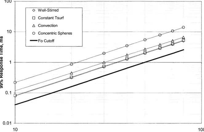
the temperature has reached 99% of it's final steady state value (or rather, 99% of the change from its initial to its final steady state value). If we then determine the time at which this occurs and do so for a range of particle sizes, we arrive at a relationship between particle size and critical time response as it shall be called (teit). This plot is shown in Figure 7. Each Equation (11), (19), (31), and (39) was solved for the critical time over a range of particle diameters.. The critical time was determined by using a secant root finding method.

As Figure 7 shows, the time response for modest size particles such as in the current investigation (50-70 pm) is on the order of 2-5 ms.

100 -0 Well-Stirred 0 Constant Tsurf A Convection 10 _{0 Concentric Spheres} E -Fo Cutoff E U) 0 0. U) 4) 0 0.1 0.0 10 100 Particle Diameter, ptm

Figure 7 - Particle Thermal Response Time.

4.2.4 Discussion and Conclusions

Detailed analysis and explanation has been presented for several different approaches to modeling the spherical PIT tracer particles for thermal response time. Commentary is presented in the body of the preceding sections, and is summarized here. The convection solution is not deemed to be appropriate, for convection is predicated on a relative motion with the surrounding fluid. Argument is made that PIV is based on the fact that the particles move with the fluid (in the immediate vicinity), and therefore there is no relative motion with the fluid in the region of interest here. The constant surface temperature condition also most likely does not apply. The physical interpretation again is of a very high convection environment. The concentric sphere method is not a good physical model, as the material surrounding the particle is in reality a fluid and not a solid. Also, the outer radius R2 is

arbitrarily determined. Putting this radius at larger and larger values continually increases the response time, as there is a larger resistance through he outer shell (i.e., gradients).

The well-stirred fluid approach is the one that makes the most sense physically. It is based on a simple energy balance of the particle and surrounding fluid. The mass of surrounding fluid can be increased, but the solution time will stop changing as this mass approaches an infinite bath. This occurs at relatively small radii, on the order of 2-5 times that of the particle itself. This is the method that is used for the remainder of the analysis, and the one that should be used for evaluating the PIT particles henceforth.

4.3 One Term Series Approximation

Regardless of the assumed boundary and initial conditions imposed on the spherical tracer particles, the mathematical solution always takes the form of an infinite series summation, as evidenced by Equations (11), (19), (31), and (39). However, these full summations are only necessary when the initial stages of transient heat transfer are involved. Heisler [14] shows that only a single term of the infinite series is sufficient for a dimensionless time, t*, greater than 0.2. Here, t* (also called the Fourier Number, Fo) is defined as

t* F =a t __4a t

t*=Fo= =d 2 ₍₄₀₎

Solving for time t we obtain,

t *-d

t * (41)

This time t sets a lower bound for the applicable range for the one-term series approximation. For a given particle size (d), a response time can be calculated using one of the four methods and equations outlined above (for a given 0). If the time calculated for a this 0 is smaller than the threshold time dictated by Equation (41), than the one-term series approximation is not valid. Greater than this threshold, and the one-term series can be utilized with little to no loss in accuracy. Figure 7 plots Equation (41), and shows that for any of the four modeling methods, the 99% response time is well above the threshold. Therefore, Equation (39) can be evaluated for only n=1 (first term).

The rationale behind choosing the 99% response time to investigate is based on the following supposition. A reasonable temperature range that is encountered in this study is approx. 25'C. In the case that a particle undergoes a step change of this amount the particle must be greater than 96% of the way to it's final state to be within less than 1PC. So for the current analysis a value for E of 0.01 (99% response time) is used.

The one-term series approximation is made not only to aid in computational efficiency and speed, but also to enable the solution to be explicitly solvable for time t. This expression for time is utilized in the following sections concerning particle size distribution.

The solution for the particle thermal response is now abbreviated using the 1-term series. For n = 1, 0(t)AVG =i1(, +1) 1 -A It (42) where AI is defined by

1

_{+ 3.(2, + 3)}

_-

_(R

_p)

₊₉

₂

_p

p)4

4.3.1 Size Distribution Effect on Time Response

Like PIV, PIT analysis divides the image into interrogation regions, and works with averaging type algorithms to arrive at temperature. It is appropriate therefore to derive an average time response value for a sub region, based on an assumed particle distribution. To do this, Equation (39) must be solved explicitly for time. The one-term approximation derived in Equation (42) enables this analysis. This result is,

_ ~ '

+i-AY

t(9,d) I -In1 (44)

ap, s(E +1)-A,)

where AI is given in Equation (43).

A certain size distribution of particles is assumed within a given image region. A

Gaussian size distribution is used here to illustrate size distribution effects. A Gaussian distribution, with mean value of m and variation (standard deviation) s takes the form

-(d-m )2

G(d)

Figure 7 illustrated the time response of individual particles of size d; smaller particles react faster than larger ones. As particle fluorescence is a function of volume, it is appropriate to calculate an average response time by weighting the individual particle time by its relative volume contribution to the population, given by Equation (45) and the volume, V. This weighting is accomplished by taking the integral over a given range of the product of population density and time, and dividing by the overall population density. That is,

d2

[t(d) -

-V(d)]dd

tAVG d2 (46)

J[G(d)

-V(d)]dd

Since the bounds for the range, di and d2, can be logically given as a function of the

mean and standard deviation, the bulk average time is only a function of m and s. As such, the equation may be looked at in terms of the relative variation to the mean, or s/m. In addition, a good measure of the necessity of including the size distribution effect on the response time is given by examining the volume weighted average time to the normal response time for a particle of size m. Figure 8 shows this relationship.

Figure 8 shows that for a distribution where there is very little deviation from the mean value (i.e., s is small), the volume distribution weighted time approaches that of the equivalent single particle response time value for a particle of size m. However, for a relatively large particle distribution spread (s large -> s/m large), the difference from a single particle time is less than becomes increasingly large. Indeed, as Figure 8 shows this relationship is exponential over the first 10-20% of s/m, and shallows out above this.

The end result is this: if a relatively small the particle distribution variation is assumed, the temporal threshold PIT validity is made simply by using the time response calculated for a particle of mean size m, given by Equation (42). If a relatively large variation is assumed (or known), then care should be taken and a reasonable threshold should be calculated using Equation (46).

100

107

0.1

1% 10% 100%

Distribution Relative Standard Deviation (s/rn)

Figure 8 - Distribution Effect on Time Response

Thermal response may be an important factor by two scenarios. First, changes in the flow field may be extremely fast and one wishes to detect the temperature changes occurring in a time on the order of the laser pulse duration. In this instance, the time response outlined above should be calculated and monitored, as there is a potential risk of misinterpretation of the results. However, if it is desired to track the time evolution of temperature changes or gradients, then subsequent frames from a typical camera capture sequence are typically analyzed. Typical high-speed CCD imaging cameras used for PIV analysis have frame rates on the order of 30-100 fps. This translates to between 10 and 33 ms from frame to frame. This is ample time for even the large, wide variation particle distributions (per above) to reach steady state.