Age-dependent capillary thinning dynamics of physically-associated salivary mucin networks

Age-dependent capillary thinning dynamics of

physically-associated salivary mucin networks

The MIT Faculty has made this article openly available. Please share

how this access benefits you. Your story matters.

Citation

Wagner, Caroline E. and Gareth H. McKinley. “Age-Dependent

Capillary Thinning Dynamics of Physically-Associated Salivary

Mucin Networks.” Journal of Rheology 61, 6 (November 2017): 1309–

1326 © 2017 The Society of Rheology

As Published

http://dx.doi.org/10.1122/1.4997598

Publisher

Society of Rheology

Version

Author's final manuscript

Citable link

http://hdl.handle.net/1721.1/119828

Terms of Use

Creative Commons Attribution-Noncommercial-Share Alike

Detailed Terms

http://creativecommons.org/licenses/by-nc-sa/4.0/

Age-dependent capillary thinning dynamics of

physically-associated salivary mucin networks

Caroline E. Wagner ∗1 and Gareth H. McKinley †1

1_{Department of Mechanical Engineering, Massachusetts Institute of Technology,} Cambridge, MA. 02139

July 10, 2017

Abstract

Human whole saliva consists of a physically-associated network of mucin molecules. The inter-chain physical associations control the rheological characteristics of the solution and in particular, the lifetime of filaments and threads. Measurements show that the shear rheology of salivary mucin solutions (as measured by steady shear viscosity and small amplitude oscillatory shear (SAOS)) is quite insensitive to sample age over a 24 hour period following sample collection. By contrast, the filament thinning dynamics vary dramatically, with the characteristic relaxation time of the saliva and the breakup time of a fluid thread decreasing significantly with sample age. We interpret our results within the framework of a Sticky Finitely Extensible Network (SFEN) model which respects the known physical dimensions and properties of the mucin molecules in saliva, and models them as a network of physically associating and finitely extensible polymer chains. The model predicts an initially strain-hardening response in the transient extensional rheology, followed by a sudden extensional thinning and filament rupture as the chains approach their maximum extensibility and the tension between junction points increases rapidly. We show that the model can accurately capture the changes observed in the filament thinning dynamics with sample age by incorporating a steady decrease in the molecular weight of the supramolecular aggregates of mucin. These experimental observations highlight the importance of considering sample age and enzymatic degradation when reporting extensional rheological measurements of saliva.

∗_{cewagner@mit.edu} †_{gareth@mit.edu}

1

Introduction

The development of a nonlinear viscoelastic constitutive model that can qualitatively describe the rheol-ogy of a sticky or physically-associating reversible network of polymer chains has applications to a wide variety of biological problems. For instance, protein and polysaccharide interactions in animal cytoskele-tons and plant cell walls, respectively, have been accurately described using Glassy Worm-Like Chain Models [1], while DNA/protein interactions and cell division are highly dependent on interactions with the surrounding tissue network [2, 3]. It is generally not possible to describe the rheology and mechanics of such complex biopolymeric systems by considering the dynamics of the constituent chains in isolation [2, 4]. However, the macroscopic rheological response of mucus and other bodily fluids has been success-fully modeled by incorporating associative network considerations (see for instance the work by Ewoldt et al. on Hagfish slime [5] or by Broedersz et al. on actin networks [6]). The ‘sticky’ elements of the bio-logical macromolecules in these systems originate from a number of different association types, including hydrogen bonding, ion complexation, disulphide linkages, and local crystallization domains [7]. Physical associations between chain segments can generally be accounted for by confining the segment ends to lie in an energy well of width rcand depth ∆G [1, 2, 4, 8] that depends on the type of interactions in the system and the level of tension in the chain segments that form the network. As the elastically active network is strained by extensional deformation and individual segments are stretched, the energy well they must overcome becomes increasingly shallow, and the rate of chain dissociation increases. This is analogous to rejuvenation concepts in soft glasses, where thermally activated jumping between local traps occurs [1].

The particular physically associating network of interest to this study is the salivary network; a glycoprotein-based hydrogel formed by a complex set of interactions between the constituent mucin chains includ-ing charge-mediated carbohydrate-carbohydrate interactions, weak calcium-mediated physical crosslinks, stronger disulphide bonds, and hydrophobic interactions [9, 10, 11]. This complex network results in saliva being highly viscoelastic, and indeed without the ability of saliva to form viscoelastic thin films, speech and swallowing would be severely impaired, and oral decay would be inevitable [10, 12, 13]. Characteri-zation and quantification of saliva viscoelasticity is also becoming increasingly important as a diagnostic tool, largely as a result of the ease and safety of obtaining fluid samples, as compared to more commonly used biofluid sources such as blood [14]. For instance, Basilevsky et al. have explored the degradation of sputum upon exposure to certain bacteria as measured through changes in its elastic properties [15], while

Zussman et al. have noted that differences in saliva viscoelasticity between teenagers and the elderly may explain why the most common dental health issues plaguing these two age groups differ [16].

As early as 1922, however, in his ground-breaking studies of saliva’s potere filante (or ‘filament forming potential’), Aggazzotti observed that the rheological properties of saliva are not constant with time [17]. In a series of experiments, he found that both the shear viscosity (as measured with a viscometer) and the extensional properties of saliva (as measured by the maximum length of a fluid filament that was formed by stretching a sample from the end of a capillary tube) decreased as the age of the sample (or time since it was extracted from the mouth) increased. He further noted that the solubility of the salivary components upon addition of acetic acid increased with sample age [17]. At the time, Aggaz-zotti attributed these observations to “changes in the physical state, the molecular constitution, of the mucin” [17]. More recent studies on the size of salivary proteins by Esser et al. [14] measured using Sur-face Enhanced Laser Desorption/Ionization Time of Flight Mass Spectrometry (SELDI-TOF-MS) have shown quantitatively that with time, enzymatic and biological activity lead to degradation of the mucin molecules contained in the saliva. Despite this, the vast majority of the literature on the shear and exten-sional rheological properties of saliva makes no mention of the age of the sample used, which, in addition to the disparity in measurement techniques, may help to explain why reported values differ so greatly [10].

In this paper, we present data on the shear properties (steady shear viscosity and SAOS measurements of the linear viscoelasticity) and extensional rheology (as measured with a Capillary Breakup Extensional Rheometer (CaBER)) of saliva at six different sample age times (0 h < tage < 24 h). We show that the

shear rheology remains largely unchanged, while the extensional properties of saliva deteriorate completely over the time period in question. We quantify these changes in the extensional rheology through the development of a Sticky Finitely Extensible Network (SFEN) model, extended from the work of Tripathi et al. for synthetic associative polymers [8], in which saliva is modeled as a physically associating network of finitely extensible elastic segments. We show that this model can accurately describe the capillary thinning and filament rupture behaviour of saliva using parameters that are consistent with the biological properties of the mucin chains. This model can systematically account for the observed temporal changes through a progressive decrease in the molecular weight of the primary polymer component (MUC5B) in the mucin network.

2

The Salivary Network

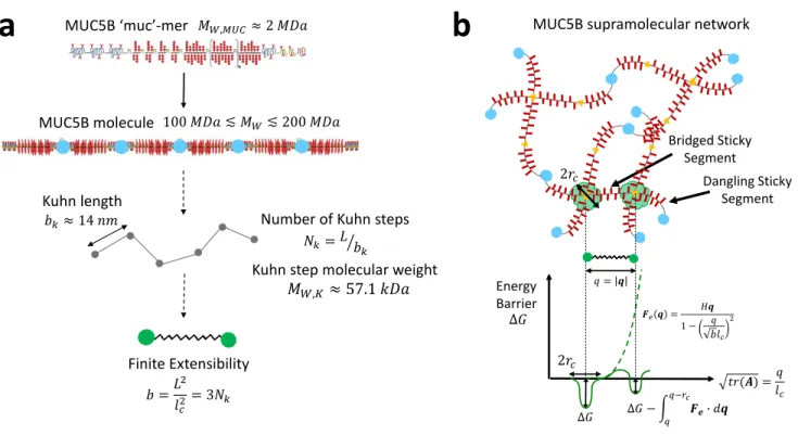
The viscoelastic properties of whole saliva can be largely attributed to its principal structural element: the high molecular weight mucin MUC5B [10], depicted schematically in Figure 1a. MUC5B is heav-ily glycosylated, with approximately 80% of its mass derived from carbohydrates forming moderately branched oligosaccharide chains that attach to the protein core in a bottlebrush configuration [18]. The intact MUC5B molecule found in secretions consists of 50− 100 macromonomer subunits [19], which we term ‘muc-mers’, each with a molecular weight of approximately MW,M U C ≈ 2 MDa [19], assembled via disulphide bonds (shown schematically as light blue filled circles in Figure 1a) in a linear fashion, leading to an overall estimated molecular weight of MW ≈ 150 MDa [19]. The overall supramolecular mucin network depicted in Figure 1b is formed by topological entanglements and hydrophobic crosslinking in-teractions between the non-glycosylated regions of these enormous biopolymers, as well as other weak associations such as ion complexation and electrostatic repulsion [10, 18].

MUC5B ‘muc’-mer

Kuhn length

Number of Kuhn steps

Kuhn step molecular weight

Finite Extensibility MUC5B molecule

MUC5B supramolecular network

a

b

Figure 1. Schematic description of the MUC5B mucin network parameters used in this paper. (a) Coarse-graining of an individual MUC5B molecule to a bead-spring chain. The schematic representa-tions of the MUC5B muc-mer and macromonomer are reproduced from [18]. (b) Organization of the MUC5B supramolecular network with both dangling and bridged sticky segments, as well as a schematic representation of the SFEN parameters relevant for considerations of network formation and inter-chain associations.

To simplify the problem, we coarse-grain the mucin macromonomer structure by approximating the chains to be random walks of Nk Kuhn steps of Kuhn length bk [20]. The persistence length of MUC5AC, which is a genetic relative of MUC5B showing significant homology in its non-glycosylated domains [21], has been estimated by Cao et al. at pH7 using Dynamic Light Scattering to be ap-proximately lp = 7 nm [22]. From this result, we can obtain an estimate for the Kuhn length of MUC5B from the relationship bk = 2lp = 14 nm. Additionally, from the fully extended MUC5B muc-mer length of Q0,M U C = Nk,M U Cbk = 500 nm measured by Kesimer et al. [19], the number of Kuhn steps per muc-mer and their molecular weight MW,k can be approximated as Nk,M U C ≈ 35 and

MW,k = MW,M U C/Nk,M U C ≈ 57.1 kDa. Finally, the finite extensibility b of an intact MUC5B molecule with nc muc-mers and a resulting molecular weight of MW = ncMW,M U C, which is defined as the square of the ratio of the fully extended chain length to its equilibrium size, can be calculated from

b = 3MW/MW,k= 3Nk [20]. This results in a finite extensibility of b≈ 8000 based on the initial molecu-lar weight of the entire MUC5B molecule, MW ≈ 150 MDa.

Following Rubinstein and Colby [23], the plateau modulus of a polymer network with well defined entan-glement and crosslink molecular weights (MW,e and MW,x respectively) is given by

G≈ ρkBNAT ( 1 MW,e + 1 MW,x ) ,

where ρ is the density of the polymer, kB is the Boltzmann constant, NA is Avogadro’s number, and T is the temperature. In the case of mucins, however, the structural and association details of the MUC5B network are not yet well understood, and consequently MW,e and MW,x are not well-defined [18, 24]. In this case, we employ the Rubinstein and Colby definition for the plateau modulus Gs of a general polymer network with apparent strand molecular weight MW,s[23], allowing us to obtain an estimate for the molecular weight of a sticky segment as

MW,s =

ckBT NA

Gs

, (1)

where c is the concentration of MUC5B which has been determined by Raynal et al. to be c = 233µg ml−1 in saliva [25]. In general, the plateau modulus of a typical biopolymeric gel is not as clearly identifiable as that for a polymer melt, GN0 [26]. Nevertheless, we can estimate Gs from SAOS data, and with this in place, the number of physical interactions, or ‘sticky’ points, per mucin macromonomer follows

immediately as z = MW/MW,s. Finally, we fix the interaction strength of these sticky sites that assemble the physically associated network at ∆G ≈ 6kBT ; an average value for weak physical interactions such as hydrophobic interactions and electrostatic repulsion [27].

With these biological parameters in place, in the section to follow, we develop a model that respects these molecular dimensions and allows us to investigate the nonlinear properties of mucin solutions, particularly at the large Hencky strain values relevant to CaBER experiments near filament breakup.

3

Model Description

We follow the approach of Tripathi et al. [8], who studied the nonlinear shear and extensional rheo-logical properties of hydrophobically modified ethoxylate-urethane (HEUR) telechelic systems, to model the salivary network. This model, extended from the ideas of Tanaka and Edwards [28, 29] and Vaccaro and Marrucci [30], is particularly suitable as it focuses specifically on the nonlinear rheological properties that dominate filament thinning measurements, and can account for a wide range of interaction types and number of interaction sites [8]. Telechelic HEUR polymers contain both hydrophilic central regions and hydrophobic end groups which physically associate with one another in flower-like micelles to mini-mize their exposure to the surrounding aqueous environment [8], introducing the ‘sticky’ character to the network. We introduce an analogous term to capture the physical interactions in the salivary network, and allow for destruction and reformation of network junctions at these points [8].

The number density of elastically active segments (meaning those that form inter-chain bridges and participate in the network) is denoted by ν and depends on the depth of the energy well ∆G through the expression [28] ν = n ( exp (∆G/kBT ) 1 + exp (∆G/kBT ) ) (2)

where n = cNA/MW,s is the total number density of sticky segments. When ∆G is large compared to the thermal energy, ν ≈ n and all chain segments are considered active and able to contribute to the accumulation of polymer stresses in the network [8].

of the natural thermal vibration frequency Ω (where 108_{Hz < Ω < 10}10_{Hz) and the quasi equilibrium}

likelihood of reaching a transition state given the activation barrier ∆G, i.e.

Ωexit= Ω exp (−∆G/kBT ). (3)

The depth of the relevant energy well ∆G under flow depends, however, on the extent to which the chain segments are stretched, which can be characterized by the end-to-end vector q of each sticky segment.

These concepts related to network formation and inter-chain associations are depicted schematically in Figure 1b.

The fraction of bridged chains as a function of chain stretch and time can be specified by a distribution function Ψa(q, t). Ψa can also be defined in terms of the probability density function ψa for a single active chain through Ψa= νaψawhere νa≤ ν is the number of bridged, elastically active chain segments

(and hence (ν− νa) is the number of dangling elastically active chain segments), and ψais normalized by

∫

ψadV = 1. Unlike Tripathi et al. [8], we consider only the bridged chains (or species A in their work)

to contribute to the stress tensor and we neglect contributions from temporarily dangling segments (or species B). Since our model allows for both network dissociation and rejoining, the number of bridged chains νa consequently varies with the state of stress in the network.

By considering the interactions of the junction points with the flow (see discussions by van den Brule and Hoogerbrugge [31] and Bird et al. [20]), the conservation equation for the probability distribution function can be written in the form of a Smoluchowski expression

∂Ψa ∂t =− ∂ ∂q · [ (∇v)T · qΨa ] − M(q, t)Ψa+ ˜L(q, t), (4)

where M (q, t) and ˜L(q, t) are the destruction and creation rate of junction points, respectively.

Multi-plying Equation (4) by the second moment tensor qq and integrating over configuration space [8] yields

⟨qq⟩(1) =−M ⟨qq⟩ + ˆLI, (5)

where ˆL = 4π/3∫₀∞Lq˜ 4_{dq [20], I is the identity tensor, and the subscript (1) denotes the upper convected}

⟨qq⟩(1) =

D⟨qq⟩

Dt − {(∇v)

T _{· ⟨qq⟩ + ⟨qq⟩ · (∇v)}. (6)}

Finally, by expressing the stretching of the network in terms of a microstructural deformation tensor defined as A = ⟨qq⟩ l2 c , (7) where lc= √ Nkbk/ √

3 is the characteristic equilibrium size of an entire network macromonomer [8], we arrive at a differential equation governing the evolution of A

A(1)=−MA + LI, (8)

where L = ˆL/l2

c. Following the approach originally proposed by Tanaka and Edwards [28, 29] and later extended by Vaccaro and Marrucci [30] and Tripathi et al. [8], we can incorporate finite extensibility mediated network behaviour by defining the network destruction rate to be the (nonlinear) product of the natural thermal vibration frequency and a stretch-dependent exit frequency, i.e.

M (q)= g(c, MW,s)Ω exp ( − 1 kBT { ∆G− ∫ q−rc q Fe· dq }) , (9a)

where g(c, MW,s) is a scaling function determined from equilibrium measurements that depends on the chain segment concentration and molecular weight and Fe(q) is the stretch-dependent tensile elastic force

acting on a segment in the network. Note that for the remainder of this manuscript, to simplify notation since the concentration and strand molecular weight are not changed during our experiments, we combine

g(c, MW,s) and the network exit rate Ωexit from Equation (3) into a single, scaled timescale associated with the lifetime of network junctions: λexit= 1/ (gΩexit). This allows us to rewrite Equation (9a) as

M (q)= 1 λexit exp ( 1 kBT {∫ q−rc q Fe· dq }) . (9b)

The upper limit of integration in Equation (9b) represents the distance that a stretched network segment with length q = |q| must be displaced through to escape the energy barrier of width rc associated

with a sticky domain, as illustrated in Figure 1b. Representing the chain segments as finitely-extensible non-linear elastic (FENE) springs, we can express the deformation-dependent force using the Warner expression [8] as Fe= Hq 1− ( q/(√blc) )2, (10)

where H = kBT /lc2 is the spring constant [32] and Q0 = √

blc is the fully extended length of the macromonomer chain. Substitution of this result into Equation (9b) and applying the usual Peterlin closure approximation allows us to arrive at an expression for the ensemble average dissociation rate

M (tr(A)) = 1 λexit  1− (√ tr(A)− X)2/b 1− tr(A)/b   b/2 , (11)

where X = rc/lc is the width of the energy barrier normalized by the equilibrium chain size and tr(A) indicates the trace.

To balance the destruction rate of elastically active segments (M (tr(A))), a creation term denoted by

L in Equation (8) is required [33]. We follow Vaccaro and Marrucci [30], as well as Ng et al. [34] and

Ewoldt et al. [5], and choose a constant stretch-independent creation term L such that under no flow conditions, the distribution is stationary with A₍₁₎ = 0. We thus obtain

L = 1 λexit [ 1−(√3− X)2/b 1− 3/b ]b/2 . (12)

which for large b≫ 3 simplifies to L ≈ λ−1_exit. The microstructural deformation tensor A is related to the polymer stress tensor τp through the Kramers expression [20]

τp =−nkT [f(tr(A))A − I], (13)

where f (tr(A)) is the FENE term that accounts for finite extensibility within the chain segments. Using the Peterlin closure approximation [20], we can write the following expression for the ensemble average stretch in the network

f (tr(A)) = 1

At equilibrium (τp = 0), Equations (13) and (14) imply that trAeq = 3/ (1 + 3/b) ≈ 3 for the large values of the finite extensibility parameter b used in this study.

Equations (8)-(14) represent a set of evolution equations for the polymeric contribution to the stress in a Sticky Finitely Extensible Network which we refer to as SFEN for compactness. The evolution equation for the number density of bridged active segments is found by integrating Equation (4) over configuration space [8], yielding

dνa

dt =−Mνa+ L(ν− νa). (15)

Further, for the specific case of a time-varying shear-free or elongational flow, the SFEN equations for the number density of bridged elastically active segments and the non-zero individual components of the microstructural deformation tensor A become:

dAzz

dt = 2 ˙ϵAzz − MAzz+ L (16)

dArr

dt =−˙ϵArr− MArr+ L (17)

where ˙ϵ(t) is the instantaneous strain rate imposed by the kinematics of the flow under consideration. For the various specific elongational flow types considered in the sections to follow, the time evolution of flow stresses are determined by solving the governing SFEN equations ((15)-(17)) in combination with the appropriate expressions for the flow kinematics, where the junction destruction, M (tr(A)), and cre-ation, L, rates are given by Equations (11) and (12), respectively. We note that in the limit of a steady state shear flow of vanishing strength, it is straightforward to show that the steady state shear viscosity predicted by the SFEN model is η0= ηs+ νkBT λexit/2, where ηs is the solvent viscosity and the steady state value of the number of bridged active chains is νa,eq = ν/2.

3.1 Response of the SFEN model under simple elongational flow conditions

To explore the nonlinear response of this model for a physically associated biopolymer network, we first consider a simple, homogeneous, elongational flow at constant strain-rate ˙ϵ0. In Figure 2a, we plot the

predicted evolution in the transient extensional viscosity η+

e = (τzz − τrr)/ ˙ϵ0 normalized by the steady

state elongational viscosity ηe,0 = 3η0 as a function of the accumulated strain ϵ = ˙ϵ0t at various values

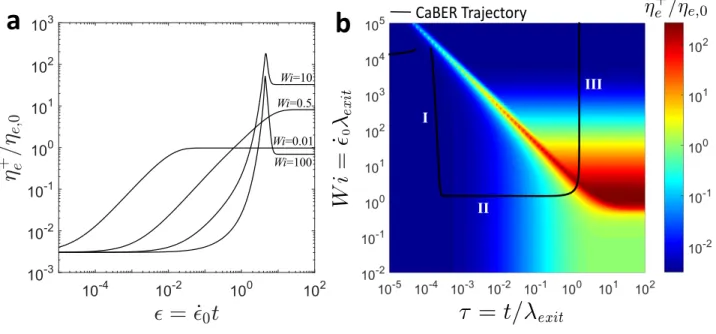
of the Weissenberg number W i = ˙ϵ0λexit. In Figure 2b, this same information is presented as a three-dimensional surface as a function of dimensionless time and Weissenberg number. The trajectories in Figure 2a correspond to horizontal lines in Figure 2b at each of the values of W i indicated.

a

b

Figure 2. (a) SFEN model predictions for the normalized extensional viscosity η_e+/ηe,0 under simple, homogeneous, elongational flow conditions at constant strain-rate ˙ϵ = ˙ϵ0 as a function of the total

accumulated strain ϵ = ˙ϵ0t for W i = ˙ϵ0λexit = 0.01, 0.5, 10, and 100. (b) Surface plot of the SFEN model predictions for the normalized extensional viscosity η_e+/ηe,0 as a function of both W i and the non-dimensionalized time τ = t/λexit under simple, homogeneous elongational flow conditions (coloured surface) as well as the trajectory followed during a filament thinning (CaBER) experiment for which ˙ϵ =− (2/R) dR/dt (solid black line). The regions indicated with roman numerals in the CaBER trajectory correspond to viscocapillary thinning (I), elastocapillary thinning (II), and the terminal thinning regime (III) [35]. In both (a) and (b), the chosen parameters correspond to those determined for saliva at

tage = 0 h in Section 4: b = 8000, X = 0.02, ∆G = 6kBT , λexit = 0.26 s, ηs/η0 = 0.003, and Ec =

νkBT /(σ/R0) = 0.02.

At time t = 0+, there are no accumulated stresses in the polymer network and consequently η_e+(t = 0+) = 3ηs, with the solvent contributing exclusively to the extensional viscosity. As the accumulated strain increases the polymeric contributions to the stress grow. For W i = ˙ϵ0λexit ≤ 0.5, the chains do not stretch sufficiently for dissociation to become significant, and the extensional viscosity plateaus at the expected equilibrium value of η_e+(t → ∞) = ηe,0 = 3η0. As the strain rate ˙ϵ0 is increased, it is clear

approximately constant value of the product (W i)c(τ ) = ( ˙ϵcλexit)(t/λexit) = ˙ϵct = ϵccorresponding to the diagonal‘line’ at approximately 45◦ formed by the surface countoursin Figure 2b. At larger strains ϵ > ϵc the extensible segments of the network begin to stretch closer to their full extent, and the nonlinear terms associated with finite extensibility and network dissociation come increasingly into play. This is seen in Figures 2a and 2b as an initial strain hardening and increase in the extensional viscosity η_e+followed by a dramatic rupture of the network and decrease of the extensional viscosity at a large Hencky strain ϵc≈ 4. We note that similar extensional viscosity overshoots in highly branched but non-physically associated LDPE networks have been modeled by Hoyle et al. [36].

3.2 Response of the SFEN model during Capillary Breakup Extensional Rheometry (CaBER)

We now consider the response of the model during a filament thinning experiment in a CaBER device. Unlike the constant homogeneous strain rates considered above, the dynamics of the problem are specified by assuming a time-varying and axisymmetric uniaxial elongational flow [vr = −1₂˙ϵ(t)r, vz = ˙ϵ(t)z] in a cylindrical filament of radius R(t), from which it follows that the time-varying strain rate is given by

˙ϵ(t) =−2

R dR

dt. (18)

Following [35], we can combine force balances in the radial and axial directions to eliminate the unknown pressure inside the thinning filament and obtain the following force balance, in which the capillary stress is balanced by a combination of the extensional stress difference resulting from the viscous solvent and the deforming and physically associated polymer network:

σ

R = 3ηs˙ϵ + (τp,zz− τp,rr), (19)

where σ is the surface tension of the fluid. Using the definition of the strain rate in Equation (18), the microstructural deformation terms Azz and Arr (Equations (16) and (17)) and the governing force balance (Equation (19)) can be written in the form

dAzz dt =− 4 R dR dtAzz − MAzz+ L, (20)

dArr dt = 2 R dR dtArr− MArr+ L, (21) σ R =− 6 R dR dt ηs+ νakBT f (Azz− Arr), (22)

where the junction destruction, M (tr(A)), and creation, L, rates are given by Equations (11) and (12), respectively.

The resulting equation set comprises a stiff initial value problem that can be integrated in time (e.g. using Matlab from R = R0and νa= νa,eqat t = 0) for different initial conditions to compare with experimental measurements (as has been done previously in [37, 38, 39, 40, 41] for other constitutive models). As the filament thins under capillary pressure, the strain rate ˙ϵ(t) given in Equation (18) and total Hencky strain ϵ(t) correspondingly evolve in time. In Figure 2b, we superimpose a CaBER trajectory (solid black line) labeled with regions (I)-(III) onto the three-dimensional extensional viscosity surface, using the same physical parameters as for the simple elongational flow curves. We must also specify an elas-tocapillary number which compares the ratio of elastic to capillary forces, and an appropriate value for mucin filaments with σ≈ 72 mN m and R0 ≈ 0.5 mm is Ec= νkBT / (σ/R0) = 0.02. We can define three

general dynamical regimes as shown in Figure 2b: (I) viscocapillary thinning during which the solvent extensional stresses predominantly balance the capillary pressure; (II) a constant strain-rate regime of elastocapillary thinning (termed the ‘middle elastic time’ by Entov and Hinch [35]) during which axial polymer stresses balance capillary pressure but the chains remain far from their finite extensibility limit (b(II) ≫ A(II)zz ≫ A(II)rr , f(II) ≈ 1); and (III) a terminal regime during which the polymers approach their maximum extension and filament rupture occurs [35]. As can be seen, following a rapid initial strain hard-ening and decrease in the strain-rate ˙ϵ associated with rapid filament thinning during the viscocapillary regime (I), the strain-rate and extensional viscosity both plateau at nearly constant values during regime II, and finally, as the chains approach their maximum extension (regime III), the elastic forces become large and the destruction rate M (tr(A)) (Equation (11)) diverges, leading to a rapid destruction of the network and filament rupture. In this final region (III) the extensional viscosity continues to decrease with increasing strain as the number of elastically active chains decrease until ultimately the extensional viscosity is reduced to the initial solvent contribution.

3.2.1 Constant strain-rate elastocapillary thinning (Regime II)

In order to use our SFEN model to interpret experimental CaBER data with salivary mucins, the sig-nificance of the filament thinning rate, typically extracted from the time constant associated with the exponential radius decay characteristic of regime II [35], must be understood in the context of the SFEN parameters.

For many moderate molecular weight systems with finite chain extensibility, there is already significant axial microstructural stretch incurred in the system by the time this regime occurs following the initial viscocapillary thinning regime (I). However the inequality Azz ≪ b still holds (see for instance Wagner, et al. [39]). Under these conditions, a Taylor series expansion can be used to simplify Equation (11) for the destruction rate to the form

M(II)(tr(A))≈ 1

λexit

[1 + δ] , (23)

where the superscript II indicates explicitly the elastocapillary regime (II) and

δ = √ tr(A)Xb b− tr(A) ≈ √ A(II)zz Xb b− A(II)zz . (24)

In the limit of infinitely extensible springs (b → ∞) or negligible sticky effects (X → 0), δ → 0. For finitely extensible springs, Wagner et al. [39] provide an implicit analytical expression for the axial mi-crostructural deformation A(II)zz at the transition point between regimes I and II, which can be used in this instance to obtain an estimate for δ during the middle elastic time (II).A more detailed explanation regarding the derivation of this approximate result for A(II)zz is provided in Appendix A. In reality, of

course, A(II)zz and hence the destruction rate M are not constant during regime II, but for moderately extensible chains this approximation is reasonable [39] and, as we will see, allows for the development of an approximate analytic expression governing the time-dependent evolution of the filament radius during this regime.

Using the approximation in Equation (23) for M and L≈ 1/λexit, Equation (15) can be solved explicitly (with the initial condition νa(t = 0) = νa,eq = ν/2) to yield

ν_a(II)(t)≈ ν 2 + δ [ δ 2exp ( −(2 + δ)t λexit ) + 1 ] ≈ ν 2 + δ, (25)

and so indeed in this regime the number density of sticky segments is approximately constant in time. The remaining ‘middle elastic time’ approximations (b ≫ A(II)zz ≫ A(II)rr , f(II) ≈ 1) allow us to simplify Equation (20) to the form

dA(II)zz dt ≈ − 4 R(II) dR(II) dt A (II) zz − 1 + δ λexit A(II)_zz , (26)

which has the solution

A(II)_zz (t)≈ ( 1 ξ(II)_(t) )4 exp ( −t(1 + δ) λexit ) (27)

given the initial conditions Azz(t = 0) = 1 and R(t = 0) = R0, where ξ(II)(t) = R(II)(t)/R0 is the

dimen-sionless radius of the filament which we seek to determine.

Finally, the governing SFEN force balance (Equation (22)) can similarly be simplified in regime II to

σ R(II) ≈ ν

(II)

a kBT A(II)zz , (28)

and by substituting Equations (25) and (27) into (28), we obtain an explicit expression for the evolution of the filament radius during the ‘middle elastic time’, or regime II:

ξ(II)(t)≈ ( Ec 2 + δ )1 3 exp ( −t(1 + δ) 3λexit ) . (29)

The longest relaxation time of a polymer solution (λ0) is typically extracted from the period of exponential

radius decay during a CaBER experiment using the expression ξ(II) ∼ exp (−t/3λ0) [35, 37]. Comparison

of this expression and Equation (29) reveals that monitoring the rate of filament decay in regime (II) given by ˙ϵ(II) _{=−(2/ξ) ˙ξ = (2/3)λ}−1

0 therefore provides a direct measure of the network junction exit rate λ−1_exit, and that these two quantities are related through the expression

˙ϵ(II)≈ 2

3(1 + δ)λ −1

exit. (30)

of bridged active segments νa does not hold, a more sophisticated analysis (presented in Appendix B) can be used to find a more accurate expression for the local filament thinning rate in regime II.

3.2.2 Terminal asymptotic behaviour (Regime III)

Finally, we consider the asymptotic behaviour of the SFEN model as the thinning filament approaches rupture and breakup. In this regime (denoted III in Figure 2b), the chains are essentially fully stretched (A(III)zz ≈ b) [35] and as such we can approximate that the time rate of change of the axial microstructural deformation vanishes ( ˙A(III)zz → 0). Consequently, the destruction rate of elastically active segments far outweighs the creation rate (i.e. M(III) ≫ L(III)). Entov and Hinch show that for a dilute suspension of FENE-P springs in this terminal regime, the FENE term approaches f(III) → 2˙ϵ(III)λ0 and each segment

essentially behaves as a fully stretched rigid rod, resulting in a constant polymeric contribution to the viscosity given by [35]

η(III)_{F EN E−P} = 2

3nkBT λ0b. (31)

Furthermore, the filament radius in this region evolves linearly as R(III)(t) = σ(tbreak− t)/(6η(III)). Considering the analogous regime in the SFEN model, for Azz ≈ b, Eq (16) reduces to ˙ϵ(III)≈ M/2 which reveals, by direct comparison with Eq (15), that

˙ϵ(III) =− 1 2νa(III)

dνa(III)

dt . (32)

Combining this result with the kinematic definition of the strain rate (Equation (18)) and integrating, we obtain that ν_a(III) = ν ∗ a R∗4 ( R(III) )4 (33)

where ν_a∗ and R∗ are the number density of bridged chains and the filament radius when this terminal regime begins. It is clear that as the filament thins and R(III) decreases the number of bridged elastically active chains decreases very rapidly.

dependent expression to that of Entov and Hinch for the evolution in the nonlinear stretching of the chains in regime III:

f(III) ≈ √ b 2X [ (2 ˙ϵλexit)2/b− 1 ] . (34)

Neglecting the radial microstructural deformation Arr and the small contribution of the solvent stress, the late-time force balance is given by

σ

R(III)_(t) ≈ ν (III)

a (t)kBT f(III)(t)A(III)zz (t). (35)

Substituting Equations (33) and (34) as well as the approximation A(III)zz ≈ b into this expression allows us to obtain an expression for the evolution of the filament radius during regime III (non-dimensionalized by its value at the start of the terminal regime, ξ(III)(t) = R(III)(t)/R∗), in terms of time non-dimensionalized by the exit rate of network segments (τ = t/λexit):

∫ 1 ξ(III) [ 1 + 1 K(ξ(III))5 ]₋b 2 dξ(III)= ∫ −dτ 4 (36)

where the constant K is given by

K = 1 2 [ ν_a∗kBT b σ/R∗ ] (√ b X ) . (37)

The first term in Equation (37), in square brackets, is proportional to the ratio of the steady state extensional stress of a dumbbell suspension [32] to the capillary pressure in the filament at the start of regime III. From the definitions of b and X, we see that the second term, in parentheses, is the ratio of the fully extended length of a network segment to the width of the energy activation barrier rc. We term the inverse of this parameter the “stickiness number”, i.e.

Sk = X/√b. (38)

When Sk is small (or when K is large), which is achieved either by having network segments that are extremely extensible (b → ∞), or by having negligibly wide junction energy wells (rc → 0), physical association effects are negligible. In this limit, Equation (36) reduces to

∫ 1 ξ(III)dξ (III)₌ ∫ −dτ 4 , (39)

and so the terminal filament thinning kinematics are exponential in nature with ξ ∼ exp (−τ/4).

Conversely, as Sk becomes larger, as achieved by either less extensible stiffer chains or a wide junction energy well, network effects are no longer negligible. In this regime, as ξ(III)→ 0, Equation (36) simplifies to ∫ Kb/2 ( ξ(III) )5b/2−1 dξ(III) = ∫ −dτ 4 , (40)

and an explicit analytical expression for the late-time decay of the filament radius can be found:

ξ(III)→ (5b/8)5b2 _K−1/5_(τcrit− τ) 2

5b, (41)

where τcrit is the non-dimensional breakup time of the filament. In practice, as a result of the difficulty of

obtaining an explicit analytic expression for τcrit in terms of the model parameters and initial conditions,

we estimate the value of this singular point numerically as the time at which the non-dimensional filament

a

Late asympto�c result for finite Sk

b

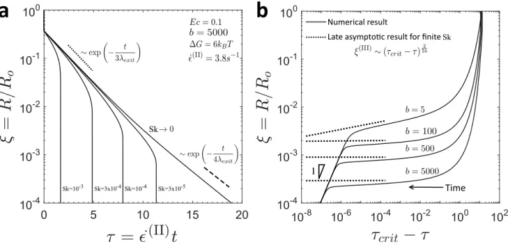
Figure 3. Filament thinning dynamics of the SFEN model, with ∆G = 6kBT , Ec= 0.1, and ˙ϵ(II) = 3.8 s−1. In (a), the effect of the stickiness number Sk on the evolution of the filament radius is shown for a value of the finite extensibility parameter comparable to those estimated for the mucin macromonomers (b = 5000). The exponential elastocapillary (II) and terminal (III) thinning regimes described in Equations (29) and (39) for the case of vanishing stickiness effects Sk → 0 are shown as the dotted and dashed lines, respectively. In (b), the asymptotic decay to breakup of the SFEN model during filament thinning experiments is shown as a function of time from the singularity (τcrit− τ) for four values of the finite extensibility parameter b with the energy well width to the equilibrium macronomer size ratio fixed at

X = 10−3. The b-dependent decay during regime III (Equation (41)) is shown as the dotted line. The final late-time linear decay of the filament radius as a result of the residual solvent contribution at very small length scales is made apparent by the indication of the region with slope 1.

In Figure 3a, the SFEN predictions for the radial evolution of a thinning filament are shown for various values of the stickiness number Sk. The exponential elastocapillary thinning regime (II) described in Equation (29) for the limit of Sk → 0 and hence δ → 0 is shown by the dotted line. Clearly, as Sk increases and network effects become large, the slope during regime (II) becomes increasingly steep, as described in Equations (30) as well as the additional discussion in Appendix B, and the filament ruptures earlier. In the limit of Sk → 0, the exponential terminal thinning dynamics described in Equation (39) are recovered, as indicated by the dashed line. In Figure 3b, the late time asymptotics of the SFEN model are shown as a function of time from the breakup singularity. Unlike the linear decay of a FENE-P filament close to rupture [35], the evolution of the filament radius for the SFEN model in regime (III) depends on the finite extensibility b of the network segments, although in practice this analytic result saturates quickly for large values of b (see Equation (41)).

When plotted in terms of Figure 3b which reflects distance from the finite time singularity corresponding to filament rupture, it is clear that there is in fact a fourth thinning regime at very small length and time scales. Once the associating mucin network has ruptured and polymer stresses have been removed, solvent stresses present the only opposition to capillary pressure and (consistent with the appropriate force balance in Equation (22)) a final universal linear decay of the filament is expected as shown in Figure 3b with a slope of unity. This decay is faster than that for a FENE-P filament (Equation (31)) as it arises from the viscous solvent alone [35]. We note here that Renardy has also investigated the breakup behaviour of fluid filaments for a number of constitutive models [42, 43, 44, 45], and our results are consistent with his conclusion that Newtonian breakup asymptotics are ultimately observed for finitely extensible dumbbell models (although the functional forms of the FENE and SFEN stretch terms do, of course, differ).

To summarize this section, we have developed a Sticky Finitely Extensible Network (SFEN) model for an associating polymeric network whose parameters respect the known biological properties of mucin molecules and whose dynamics can be related to the filament thinning theory traditionally used to interpret CaBER experimental data. Interestingly, the terminal dynamics of this model depend on the finite extensibility b of the network segments and on a dimensionless stickiness number Sk that

incorporates the width of the energy well and the length of the chains (c.f. Equations (11) and (38)).

With this analysis in place, we proceed in the following section to compare the predictions of the SFEN model during CaBER filament thinning with experimental data of saliva at various sample ages tage, and use these results to comment on the effect of enzymatic degradation on reported measures of saliva extensional rheology.

4

Results and Discussion

Saliva samples used in this paper were obtained without stimulation following the procedure outlined in [46]. Donors were instructed to refrain from eating or drinking for one hour prior to collection. Vacuum was drawn in a closed collection vial using an Amersham VacuGene Pump, into which a tube terminating in the donor’s mouth was inserted, and saliva was allowed to accumulate. Once collected, the saliva was not treated and was stored at room temperature. All shear rheology tests were performed using a stress controlled ARG2 rheometer (TA Instruments, New Castle, DE, USA) with a 60 mm, 2◦ cone-and-plate

fixture on a Peltier plate at a constant temperature T = 25◦C. Extensional rheometry tests were per-formed using a Capillary Breakup Extensional Rheometer (CaBER, Cambridge Polymer Group) with plate diameter D = 6 mm, initial plate separation Li = 2 mm and final plate separation Lf = 9.1 mm. The top plate reached its final height in a strike time of tstrike = 50 ms using a stepper motor, and the diameter of the resulting filament was tracked using a laser micrometer with a resolution of 10µm. In Figure 4a, the results of CaBER experiments are shown for measurements taken immediately after sample procurement, as well as after the sample had been sitting (untreated, at room temperature) for

tage = 1, 3, 5, and 10 h. Data for the sample at tage= 24 h are not shown since samples at that age were unable to form filaments that persisted beyond the plate strike time of tstrike = 50ms. Consistent with previous data from Zussman et al. [16], the experimental results show a clear exponential thinning region (regime II) followed by rapid filament failure (regime III).

a

b

c

SFEN model Symbols: CaBER data

0 hours 3 hours 1 hour

10 hours 5 hours

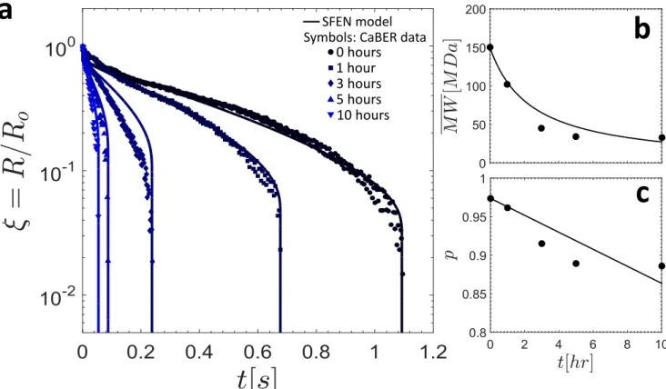
Figure 4. (a) Comparison of the SFEN model predictions with CaBER data for saliva at various sample ages. In (b) and (c), the fitted values for the weight averaged macromonomer molecular weight MW and the reaction probability p, respectively, are shown as filled circles, and the theoretical predictions for the same parameters obtained using a randomly initiated depolymerization model are shown as the solid lines.

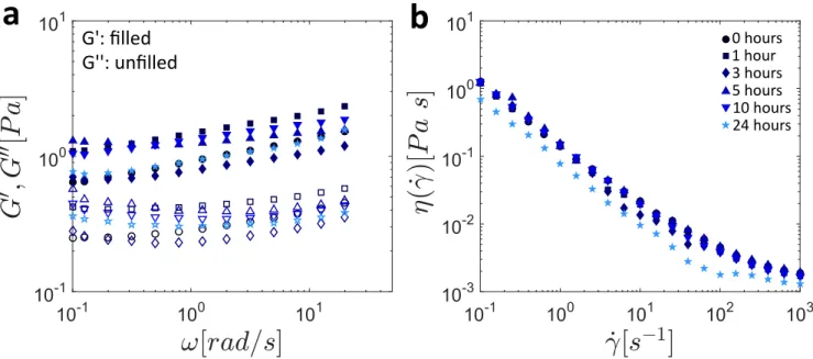
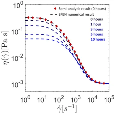
In Figure 5, the results of SAOS experiments (Figure 5a) and steady state flow (Figure 5b) for the same samples discussed in Figure 4a as well as the sample at tage= 24 h are presented. Small variations (less than a factor of 2) are observed between the samples, and appear to be more likely attributable to sample inhomogeneity than clearly discernible trends with sample age. A more detailed discussion of the steady state flow data shown in Figure 5b and the predictions of the SFEN model in steady simple shearing flow is presented in Appendix C.

a

G': filled

G'': unfilled

b

Figure 5. The shear rheology of whole saliva as measured by (a) small amplitude oscillatory shear (SAOS) and (b) steady simple shear flow. In Appendix C we show that in the shear-thinning regime, the SFEN model predictions are only weakly dependent on the sample age (set using the appropriate parameters from Table II), in agreement with our experimental observations.

The dependence of the moduli on the angular frequency, shown in Figure 5a, is nearly power-law like in nature; a signature of physically associated biopolymer networks with very large numbers of interaction modes [47]. As a result, no clear unique plateau value of the storage modulus can be defined (as expected [26]), and so we take as an approximate value Gs ≈ 2.5 ± 0.5 Pa for all sample ages. Using Equation (1), this fixes the molecular weight of each sticky segment at MW,s ≈ 2.3 × 105Da, which results in approximately z = 9 sticky segments per muc-mer. In all cases, as seen in Figure 5b, saliva viscosity is quite strongly shear thinning (with a power law index n ≈ 0.11) with no evidence of a plateau viscosity at low shear rates, and an asymptotic solvent viscosity of ηs≈ 10−3Pa s. We note that this broad power-law frequency dependence can be described quantitatively in compact form using the fractional Maxwell model, as has been recently shown in [48].

Further, recognizing that the real mucin system is polydisperse [14], we define the initial, mass-averaged, molecular weight of an entire MUC5B molecule as ⟨MW(tage = 0)⟩ = MW(tage = 0) = 150 MDa [19], where⟨...⟩ denotes an ensemble average. The width of the energy wells rcis obtained by manually fitting the SFEN model to the experimental data in order to achieve a consistent filament breakup time using the fixed, remaining parameters at tage= 0 h. The obtained result of rc= 8.35 nm is consistent with ex-perimental data from Israelachvili and Pashley on the distance over which the strength of a hydrophobic interaction decays exponentially (l ≈ 10 nm) [49] as well as the Debye length for electrostatic interactions in biological systems (l ≈ 1 − 3 nm) [50]. Finally, the rate of filament decay in regime II (˙ϵ(II)) for each saliva sample is obtained by fitting the exponential thinning region of the appropriate CaBER data set in Figure 4a to the expression ξ(II) _∼exp(₋˙ϵ(II)

2 t

) .

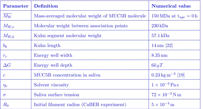
Using the shear rheological data presented in Figure 5 along with the various parameter definitions from this and previous sections, we can define the full set of 10 parameters needed for the SFEN model, which we use to fit the CaBER data in Figure 4a. These parameters are summarized in Table I, and their numerical values are provided. In Appendix D, we investigate the effect of varying a subset of these physical parameters on the filament thinning dynamics.

TABLE I. List of SFEN model parameters, along with their definitions and numerical values. The effect of varying a subset of these parameters on the filament thinning dynamics is considered in Appendix D.

Parameter Definition Numerical value

MW Mass-averaged molecular weight of MUC5B molecule 150 MDa at tage= 0 h

MW,s Molecular weight between association points 230 kDa

MW,k Kuhn segment molecular weight 57.1 kDa

bk Kuhn length 14 nm [22]

rc Energy well width 8.35 nm

∆G Energy well depth 6kBT

c MUC5B concentration in saliva 0.23 kg m−3 [19]

ηs Solvent viscosity 1× 10−3Pa s

σ Saliva surface tension 72× 10−3N m

In Figure 4a, the filament thinning predictions of the SFEN model are compared with CaBER data at various sample ages. The CaBER data is collected from the time that the plate separation has occurred (and hence the time reported is actually (t− tstrike) to be consistent with the model), and the measured radius is normalized by the filament radius R0at the time the plates have separated. The initial condition

for the filament radius of the SFEN model is taken to be R(t = 0) = R0, but since the model does not

account for the initial plate separation period, the initial axial microstructural stretch is taken to be slightly larger than the equilibrium value of Azz = 1 but still much smaller than the maximum value of the finite extensibility parameter b, namely A0_zz/b≈ 0.05. The initial radial microstructural deformation

value is set to the equilibrium value of A0_rr = 1 and all chains are assumed to be in their equilibrium configuration such that νa(t = 0) = νa,eq= ν/2. Visual inspection confirms that Equation (30) provides a good estimate for the network junction rate λ−1_exit for the first two age points (tage = 0 h and tage= 1 h), but at later sample ages when the extensibility is reduced a higher order estimate is needed (see the discussion in Appendix B). For both expressions, we use the implicit expression for A(II)zz at the transition between regimes (I) and (II) provided in [39] to approximate δ and hence the destruction rate M , where we take the polymer viscosity to be ηp = νkBT /(3 ˙ϵ(II)).

Esser et al. have shown that the distribution of protein molecular weight in saliva is highly sensitive to sample age as a result of enzymatic activity and protein breakdown [14]. Consequently, we hypothesized that the dramatic decrease in elasticity observed in the filament thinning data shown in Figure 4a as the saliva samples age could be attributed to a time-dependent decrease in the mass-averaged molecular weight of the mucin molecules. For tage > 0 h, the same procedure previously described was used to fit the mass-averaged molecular weight MW(t) for all of the sample ages considered. In so doing, we assume that the width of the activation barrier rc measured at tage = 0 h as well as all other parameters except for the finite extensibility (b = 3MW/Mk) and the network exit junction rate λ−1exit remained constant with age. The fitted results for MW(t) are shown as the solid circles in Figure 4b, and a summary of the age-dependent SFEN model parameters at all sample ages is provided in Table II.

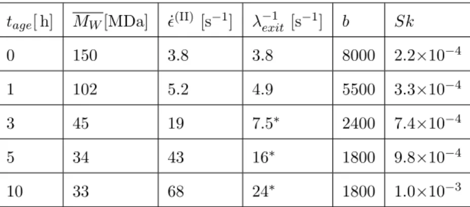
TABLE II. Age-dependent SFEN model parameters for saliva. For stickiness numbers Sk & 5.0 × 10−4, the higher order approximation relating the network junction exit rate (λ−1_exit) to the rate of filament decay in regime II ( ˙ϵ(II)) presented in Appendix B was used. These values are indicated by an asterisk.

tage[ h] MW[MDa] ˙ϵ(II) [s−1] λ−1_exit [s−1] b Sk

0 150 3.8 3.8 8000 2.2×10−4

1 102 5.2 4.9 5500 3.3×10−4

3 45 19 7.5∗ 2400 7.4×10−4

5 34 43 16∗ 1800 9.8×10−4

10 33 68 24∗ 1800 1.0×10−3

It is clear from Table II that the finite extensibility of the elastic network strands decreases dramatically with age (b∼ MW), and this increases the nonlinearity in the FENE springs which then increases the exit rate of chains from the associative network (c.f. Equation (11)). This is confirmed by the experimental observation of a strong dependence of the extensional properties of saliva on sample age, as measured by both the rate of filament thinning in the intermediate elastic time (see Table II and Equation (30)) and the time to breakup for the data CaBER presented in Figure 4a. By contrast, in the shear thinning reimge the shear rheology is relatively age-invariant as seen in Figure 5. This latter finding, discussed in

addi-tional detail in Appendix C, could be related to the fact that while the chains shorten due to enzymatic

activity, the concentration of mucin remains constant, and hence shear measurements at moderate strain values remain largely unaffected as the product (cMW) is unchanged. Our SFEN model is able to capture the evolution in the extensional viscosity through allowing a single parameter (MW(t)) to decrease with sample age. The very rapid rupture of the filament just before breakup at young sample ages is quite distinct from that observed in high molecular weight polymer solutions, and is also well described by the model through the incorporation of the stretch-dependent dissociation term (see Equation (11)). Indeed, for young samples (small tage), the mass-averaged molecular weight MW and hence the finite extensibility parameter b are large, resulting in a small value of the stickiness number Sk (Equation (38)). Consistent with Figure 3a, the thinning filaments are able to persist for longer, but their eventual breakup is more dramatic and sudden. Conversely, following degradation, the relatively less extensible mucin chains lead to larger values of Sk, and the lifetime of the filaments correspondingly decreases.

depolymer-ization [51] process of the concatenated muc-mers. Indeed, the assembly (or disassembly in our case) of supramolecular networks is often analyzed in the framework of classical polymerization theory (see the book chapter by Anthamatten [52] for additional details). In a step growth polymerization process, the weight fraction distribution of molecules ncmuc-mers in length is given by Wc(nc) = nc(1−p)2pnc−1 [53], where p is the degree of polymerization. From this definition, it follows that the mass-averaged, most probable number of concatenated muc-mers in a molecule is given by

n∗_c =∑ nc

ncWc= (1 + p)/(1− p). (42)

Using the fitted values of the mass averaged molecular weight MW = n∗c× MW,M U C from Table II, the degree of polymerization p can be found at each sample age time point tage using this formula. These results are shown as solid circles in Figure 4c.

For randomly initiated depolymerization in which complete degradation of all molecules is expected, MacCallum [51] has shown that the reaction probability p can be approximated to vary linearly in time as p(t) = p0−αt, where α is the degradation rate and p0 is the initial degree of polymerization. Although

the exact magnitude of α depends on the initial distribution of polymer molecular weights, this simple linear relationship holds even without such information [51]. From this result and Equation (42), it is straightforward to obtain that the mass-averaged molecular weight of the mucin molecules should vary in time as MW(t) = MW,M U C [ 1 + ₁ 2 p0−αt− 1 ] . (43)

These predicted expressions for p(t) and MW(t) are fit to the experimental data and shown as the solid lines in Figures 4b and 4c. From these fits, we obtain an estimate for the muc-mer degradation rate as

α = 0.011 h−1, and p0 = 0.97.

5

Conclusion

In conclusion, we have shown that the transient extensional rheology of whole saliva (as measured with CaBER) is extremely sensitive to sample age (Figure 4a), while the corresponding shear rheological

prop-erties (SAOS and steady state flow, as shown in Figures 5a and 5b respectively) are relatively invariant. In order to explain these observations, we have developed a Sticky Finitely Extensible Network (SFEN) model based on the approach of Tripathi et al. [8], which respects the known biological dimensions of mucins, and models saliva as an associating network of finitely extensible elastic segments. This model incorporates linear viscoelasticity as well as filament thinning and network rupture, and is likely to prove useful for modeling a number of biopolymeric networks under various flow conditions. Capillary thinning experiments prove particularly useful because we show (c.f. Equation (30)) that the rate of filament thinning during regime II is a direct measure of the exit rate of chain segments from the network. The stretch-dependence of this exit rate is taken into account by the SFEN model and results in progressively faster network rupture as the filament thins.

By assuming a decrease in the mass-averaged molecular weight of the MUC5B molecules with sample age (consistent with salivary measurements of enzymatic activity and protein degradation [14]), the fi-nite extensibility b of the network chains decreases as well, resulting in an increase in the importance of supramolecular network effects, which are quantified by a newly-introduced stickiness parameter Sk. Increasing values of Sk lead to more rapid growth in elastic stresses and sudden rupture of the network as shown in Figures 3a and 4a. This final rupture is much faster than the rate of thinning predicted by the FENE-P model for extensible polymer solutions [35, 37].

Our measurements and corresponding model for the evolution in network extensibility and molecular weight demonstrate the importance of carefully monitoring and stating sample age in reports of saliva and mucin network rheology. This provides a plausible explanation for why previous rheological data on saliva reported in the literature varies so greatly, and emphasizes the care that should be taken in interpreting diagnostic information from rheological measurements of saliva if sample age and degradation are not accounted for.

6

Acknowledgements

The authors would like to thank K. Ribbeck, B.Turner and M. Rubinstein for helpful discussions regarding the biological intricacies of mucin solutions. CW thanks FQRNT (Canada) for a Bourse B-1 Maˆıtrise Award. GHM would like to thank Procter & Gamble and Axalta Coating Systems for their financial

support of studies in the filament thinning of complex structured fluids.

A

Appendix A: Determination of the microstructural deformation at

the transition point between regimes I and II

In a previous study of the filament thinning dynamics of FENE-P fluids, Wagner et al. [39] have provided an implicit analytic expression for the axial microstructural deformation A∗_zz at the transition between the viscocapillary filament thinning regime (I) and the elastocapillary regime (II). This result is constructed by equating the expressions for the filament thinning rate ˙ϵ and the axial microstructural deformation Azz during regimes I and II at the transition time t∗ between the two regimes, as illustrated in Figure 6a.

a

b

I

II

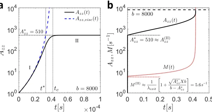
Figure 6. (a) Evolution of the axial microstructural deformation Azz (solid black curve) near the transition

time t∗ between regimes I and II. The curve corresponding to the analytic expression for Azz during the

viscocapillary regime (Equation (A.3)) is shown as the dashed blue line, and the approximate value of A∗_zz calculated using the method outlined in Wagner et al. [39] is shown as the black dashed-dotted line. (b) Full temporal evolution of Azz (solid black line) and the network junction destruction rate M (dotted

red line) for the model parameters in Table II corresponding to tage= 0 h (b = 8000, λ−1exit= 3.8 s−1). The

value of the finite extensibility b = 8000 is shown as the black dashed line, and the approximate values of A(II)zz and M(II) at the crossover from regime I to regime II are shown as the dashed-dotted black and

red lines, respectively.

viscous stress of the solvent presents the primary opposition to capillary pressure, and hence Equation (22) can be approximated as

σ

R = 3ηs˙ϵvisc. (A.1)

For a low viscosity solvent such as water, this results in a high initial rate of thinning. At the critical time

t∗ when regime II begins and viscous and polymer stresses are of the same order, Equation (A.1) must

hold simultaneously with the complete force balance (suitably modified to account for the previously outlined assumptions valid in the case of negligible sticky effects: b≫ Azz ≫ Arr, f ≈ 1 [35]):

σ

R = 3ηs˙ϵ

∗_{+ ν}

akBT A∗zz, (A.2)

which implies that the strain rate must drop in regime II to some lower value ˙ϵ∗ < ˙ϵ∗_visc. Furthermore, the

axial microstructural deformation at the transition time t∗ must be continuous between both regimes. It

is straightforward to show using Equation (20) from the main text (with M = L = λ−1_exit) that during the viscocapillary regime (I), the evolution equation for Azz is given by

Azz,visc= ( tc tc− t )4 exp ( − t λexit ) , (A.3)

where tc is the breakup time of a purely Newtonian fluid tc = 6ηsR0/σ [39] and λexit is the lifetime of

network junctions as defined in Equation (30). This result is shown as the dashed blue line in Figure 6a, while the full numerical solution of Azz is shown as the solid black curve. Additionally, as seen in Figure

6a, at the onset of regime II when sticky effects are still negligible, the rate of change of Azz is very small.

Hence, using the assumption dAzz/dt ≈ 0 and the FENE-P evolution equation for Azz, Wagner et al.

[39] show that the axial microstructural deformation at the transition between regimes I and II can be written as Azz = b ( 1− 1 2λexit˙ϵ∗ ) . (A.4)

Although the FENE-P and SFEN evolution equations for Azz differ (as a result of the incorporation of the

network junction destruction (M ) and reformation (L) terms in the case of the latter model), numerical simulations reveal that in regime I and early in regime II, before chain stretching and network dissociation effects become important, the approximation in Equation (A.4) is also reasonable for the SFEN model.

Therefore, combining and rearranging Equations (A.1)-(A.4), an implicit result for the transition time t∗ can be found as:

1 2 ( 1−exp (− t∗ λexit) b ( tc tc− t∗ )4)−1 = 2λexit (tc−t∗)+ νakBT bλexit 3ηs 1 +2νakBT bλexit 3ηs . (A.5)

Solving this expression numerically for t∗ and inserting the result into Equation (A.3) yields the

de-sired value of A∗_zz. For the conditions at tage = 0 h given in Table II, we find that A∗zz ≈ 510 and

t∗ ≈ 0.33 × 10−4 s. The elastocapillary thinning regime (II) is thus entered very quickly.

In Figure 6b, the full temporal evolution of Azz is shown for the parameters corresponding to tage= 0 h

in Table II as the solid black curve. We note that in order to clearly illustrate the expected evolution of Azz during all filament thinning regimes in Figure 6b, Azz was initialized at its true equilibrium value

of Azz(t = 0) = 1 as opposed to the slightly higher value chosen in Figure 4a that accounts for the

axial microstructural deformation incurred during the initial period of plate separation during CaBER

experiments (which is not accounted for in this asymptotic analysis). As can be seen, the value of A∗_zz

calculated implicitly provides an excellent approximation for the value of the axial microstructural

defor-mation at the transition point between regimes I and II. Further, the maximum value of Azz at filament

breakup is the finite extensibility b (shown by the dashed black line), as expected.

In order to demonstrate how this result is useful for determining the chain segment destruction rate

during regime II (denoted M(II) _{in Section 3.2.1 of the main text), we also plot the evolution of M in}

Figure 6b as the dotted red line. As can be seen, the assumption of a nearly constant destruction rate M(II) during this regime (calculated using the result for A∗_zz as well as Equations (23) and (24)) is a reasonable one, and the quantitative agreement between the the full numerical solution for M during

regime II and the approximate value of M(II) is quite good. Without the use of Equations 23 and 24, the

B

Appendix B: Filament thinning rate in the limit of large sticky

effects

We begin by noting that Equation (24) can be rewritten in terms of our new stickiness parameter defined in Equation (38): δ = √ A(II)zz b 1− A(II)zz /b Sk = √ A(II)zz /b 1− A(II)zz /b (bSk) . (B.1)

As sticky effects become increasingly important, the Taylor series expansion for the destruction rate M and the predicted near time-invariance of the number density of bridged sticky segments νa (Equations (23) and (25), respectively) become less and less accurate. Although the first effect is difficult to mitigate due to the large values of b relevant to the biological system in this study, it is possible to address the second and in doing so improve our analytic result during regime II by recognizing that in the limit of large sticky effects, the product of the stress-dependent network dissociation term M and the number density of bridged segments νa dominates over the product of the rejoining term L and the number density of dangling segments (ν− νa). As such, Equation (15) is better approximated as

dνa(II)

dt ≈ −

(1 + δ)

λexit

ν_a(II), (B.2)

which can readily be solved to yield

ν_a(II)(t)≈ ν 2exp ( −t(1 + δ) λexit ) (B.3)

using the same initial condition as before of νa(t = 0) = νa,eq = ν/2. In this case, substitution of Equations (B.3) and (27) into (28) yields a similar expression for the evolution of the filament radius during regime II ξ(II)(t)≈ ( Ec 2 )1 3 exp ( −2(1 + δ)t 3λexit ) , (B.4)

although it is clear that now the rate of filament thinning is increased due to sticky finitely extensible segments being pulled out of the network. The network junction exit rate and the filament thinning rate are hence related through: