HAL Id: hal-03197727
https://hal.inrae.fr/hal-03197727
Submitted on 14 Apr 2021
HAL is a multi-disciplinary open access
archive for the deposit and dissemination of
sci-entific research documents, whether they are
pub-lished or not. The documents may come from
teaching and research institutions in France or
abroad, or from public or private research centers.
L’archive ouverte pluridisciplinaire HAL, est
destinée au dépôt et à la diffusion de documents
scientifiques de niveau recherche, publiés ou non,
émanant des établissements d’enseignement et de
recherche français ou étrangers, des laboratoires
publics ou privés.
Distributed under a Creative Commons Attribution - NonCommercial - NoDerivatives| 4.0
Curve number calibration for measuring impacts of land
management in sub-humid Ethiopia
Habtamu Assaye, Jan Nyssen, Jean Poesen, Hanibal Lemma, Derege Tsegaye
Meshesha, Alemayehu Wassie, Enyew Adgo, Amaury Frankl
To cite this version:
Habtamu Assaye, Jan Nyssen, Jean Poesen, Hanibal Lemma, Derege Tsegaye Meshesha, et al.. Curve
number calibration for measuring impacts of land management in sub-humid Ethiopia. Journal of
Hydrology: Regional Studies, Elsevier, 2021, 35, �10.1016/j.ejrh.2021.100819�. �hal-03197727�
Journal of Hydrology: Regional Studies 35 (2021) 100819
2214-5818/© 2021 The Authors. Published by Elsevier B.V. This is an open access article under the CC BY-NC-ND license (http://creativecommons.org/licenses/by-nc-nd/4.0/).
Curve number calibration for measuring impacts of land
management in sub-humid Ethiopia
Habtamu Assaye
a,b,*
, Jan Nyssen
a, Jean Poesen
c,d, Hanibal Lemma
b,
Derege Tsegaye Meshesha
b, Alemayehu Wassie
b, Enyew Adgo
b, Amaury Frankl
a,eaDepartment of Geography, Ghent University, Ghent, Belgium
bDepartment of Natural Resource Management, Bahir Dar University, Bahir Dar, Ethiopia cDepartment of Earth and Environmental Sciences, KU Leuven, Heverlee, Belgium
dFaculty of Earth Sciences and Spatial Management, Maria-Curie Sklodowska University, Lublin, Poland eINRAE, AMAP, IRD, CIRAD, CNRS, University Montpellier, Montpellier, France
A R T I C L E I N F O Keywords: Abstraction ratio Catchment Curve number Event-based runoff Lake Tana Basin
A B S T R A C T
Study Region: We investigate the event runoff response in six sub-catchments in the Lake Tana sub- basin, headwater of the Blue Nile basin, northwest Ethiopia. Steep and mountainous terrains surround floodplains, imposing runoff and soil erosion in the upper catchments and flooding and sedimentation at floodplains. This study was conducted in the upland runoff source catchments. Study Focus: The focus is to investigate catchment characteristics that control the event runoff response in upland catchments, and how recent land management practices may have contributed to improved hydrological conditions. Event rainfall and runoff data were obtained at five-minute time steps through automated divers and tipping bucket rain gauges and related to catchment characteristics.
New Hydrological Insights for the Region: Our results show that the catchment event quickflow response was controlled by different factors of both natural and anthropogenic nature of which forest and shrubs, bund density and soil organic matter content were found to be the most important to reduce event quickflow. On the contrary, increase in cropland area caused an in-crease in quickflow. Through least square fitting procedure of the Natural Resources Conservation Service Curve Number method (NRCS-CN), a site specific abstraction ratio (λ) value of 0.01, rather than the commonly used 0.2 or 0.05, was found to be most appropriate for the sub-humid highlands of Ethiopia.
1. Introduction
The generation of surface runoff is a complex process controlled by catchment characteristics, including land use and management, soil, topography, and lithology (Sitterson et al., 2017; Zhang et al., 2018). It is a hydrological process that has a high degree of temporal and spatial variability (de Vente and Poesen, 2005; Lemma et al., 2018, 2019a). For instance, the hydrological response of small catchments is mostly different and more variable than that of large catchments (Pilgrim et al., 1982). While runoff processes are relatively well understood at the plot scale, the runoff generated from small catchments (i.e. 1–100 ha) is rather complex and
* Corresponding author at: Department of Geography, Ghent University, Ghent, Belgium. E-mail address: HabtamuAssaye.Deffersha@ugent.be (H. Assaye).
Contents lists available at ScienceDirect
Journal of Hydrology: Regional Studies
journal homepage: www.elsevier.com/locate/ejrh
https://doi.org/10.1016/j.ejrh.2021.100819
underrepresented in hydrological studies (de Vente and Poesen, 2005; Johansson, 1994; Poesen, 2018). The complexity of the hy-drological response of small catchments is partly due to the effect of variations in routing and connectivity of the different units (Boardman, 2018; Heckmann et al., 2018), but also to interactions of surface and sub-surface hydrological processes, which become more important at catchment-scales (Rodríguez-Blanco et al., 2012). Therefore, it is vital to enhance our understanding of how small catchments behave hydrologically, based on empirical studies such as those presented here.
A critical issue that remains is how land use change and land management interventions affect catchment hydrology. Measures taken in catchments may have a key objective in reducing soil erosion and sediment yield. Both are driven by the runoff response of land and stream dynamics (Boardman, 2018; Vanmaercke et al., 2014a). For example, in Rwanda, conversion of forests and grasslands to croplands has increased annual runoff (Karamage et al., 2017). Similarly, in the Blue Nile Basin of Ethiopia, foreseen land use change scenarios are predicted to increase runoff (Lemann et al., 2019). Forest losses in East Africa have increased annual river discharge and surface runoff by 16 % and 45 %, respectively (Guzha, 2018). Furthermore, management interventions have strong implications for the hydrological responses of catchments. Deep tillage practices, which break hardpan formations, increase infiltration, and reduce runoff as compared to conventional and no-tillage practices (Hussein et al., 2019). Soil and water conservation practices generally reduce runoff by 13–71 % in Africa (Sultan et al., 2017; Vanmaercke et al., 2014b; Wolka et al., 2018).
Runoff discharge from small catchments is often not directly measured, but estimated, using models such as the Natural Resources Conservation Service Curve Number (NRCS-CN). The NRCS-CN is an empirical model widely used to predict runoff using few catchment characteristics, including the Hydrologic Soil Group (HSG), land cover, and antecedent soil moisture conditions (Hawkins, 1993; Mishra and Singh, 2003; NRCS, 1997). Therefore, it has been widely used in tropical regions in general, and Ethiopia in particular (Gebresellassie, 2017; Sultan et al., 2017). However, the abstraction ratio (λ), a parameter that was initially set to be 0.2 and later recommended to be 0.05 (Woodward et al., 2003a), remains a point of concern. Studies carried out in different parts of the world (e.g. Descheemaeker et al., 2008; Fu, 2016; Hawkins, 1993; Kamuju, 2015; Mishra and Singh, 2003; Sultan et al., 2017; Woodward et al., 2003b; Gebresellassie, 2017) reported that λ varies in the range of 0 and 0.3. Therefore, analysis of the abstraction ratio from measured rainfall–runoff data will enhance the accuracy of runoff estimation (Woodward et al., 2003a), and provide further insights into the applicability of the NRCS-CN model in similar areas. As the NRCS-CN model is also integrated with other physically distributed models, such as the Soil and Water Assessment Tool (SWAT), the determination of appropriate λ values is of paramount importance in quantifying runoff for future water resource development.
In the Lake Tana Basin, runoff and erosion in the upper catchments, and flooding and sedimentation in the lowland areas, are severe challenges to sustainable development (Abate et al., 2015; Dessie et al., 2014; Lemma et al., 2019b). In addition, population growth is
fast and associated changes in land use and management are rapid (Bruin et al., 2015; Minale, 2013). Extensive use of traditional seasonal drainage ditches in cropland (feses) resulted in more runoff and a lowering of the topographic threshold for gully head development (Monsieurs et al., 2015). Significant reductions in runoff at the plot-scale have been reported due to the implementation of soil and water conservation structures, such as soil bunds, along the contour (e.g. Sultan et al., 2017; Ebabu et al., 2019). Large efforts have been made to improve catchment characteristics towards controlling fluxes of water and sediment to Lake Tana. Therefore, we examined the impact of such improvements on the runoff response of small (< 100 ha) upland catchments in this basin. The objectives of this study were to better understand the hydrological response of small catchments, fine-tune the site-specific abstraction ratio (λ) of NRCS-CN and thereby investigate how recent land management efforts may have contributed to improved hydrological conditions.
2. Study area description
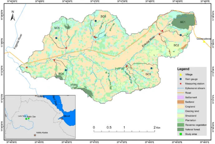
This study was conducted in the Enkulal catchment (Fig. 1), in the headwaters of the Gumara River, eastern Lake Tana Basin (11º37
to 11º39′N and 35º46′to 37º49′E). The catchment covers an area of 10.4 km2 with an elevation ranging from 2229 to 2561 m a.s.l.
According to the K¨oppen-Geiger climate classification (Peel et al., 2007), the climate of the area is temperate (Cs type), where most precipitation falls during April–September, while October–March is defined as summer, being warmer than the April–September. Average annual rainfall is 1250 mm, average annual reference evapotranspiration is ca. 1460 mm, and the daily average air tem-perature ranges 18–25 ºC (Adem et al., 2017; Temesgen et al., 2014). The geology of the area is predominantly basalt, although
volcanic ash deposits (ignimbrite) are observed along the ridges and steep slopes (Poppe et al., 2013). Most of the catchment is covered by Luvisols and Leptosols (Colot, 2012). Rainfed crop production is the primary means of livelihood (Temesgen et al., 2014) and the main crops cultivated in the area include teff (Eragrostis teff), maize (Zea mays), barley (Hordeum vulgare), wheat (Triticum aestivum), pearl millet (Pennisetum glaucum), and potato (Solanum tuberosum). In addition, the Faba bean (Vicia faba L.), white lupin (Lupinus
albus), and Ethiopian cabbage (Brassica abbysinicum) are cultivated, mostly integrated with other crops, to enhance soil fertility and to
obtain additional food and income. Eucalyptus (Eucalyptus globulus and Eucalyptus saligna) plantations have also expanded rapidly in recent years and are becoming an important source of income for farmers. Land degradation is a widespread problem caused by deforestation, overgrazing, and poor catchment management (Frankl et al., 2019; Lemma et al., 2019b). Although this area is iden-tified as a priority area for water resource development, it is also a hotspot area for soil erosion (Lemma et al., 2019b; Setegn et al., 2009) and sediment yield (Vanmaercke et al., 2014a). A wide range of sustainable land management interventions, including stone bunds, check dams, trenches, area closure and tree planting, were undertaken by the Integrated Tana-Beles Watershed Management Project, which was part of the Growth and Transformation Plan (MoFED, 2010; NPC, 2015). Recently, the UN-REDD + project, under the ‘Climate Resilient Green Economy Strategy of Ethiopia (FDRE, 2011)’, is undertaking wide-scale tree planting.
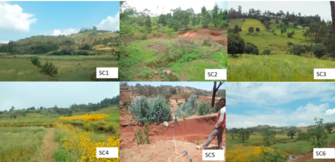
Fig. 2. Overview of sub-catchments (SC1-SC6) examined in the present study, showing differences in land cover. SC1: a natural forest covers 38 %
of the catchment; SC2: vegetation rehabilitation on steep slope; SC3: scattered eucalyptus woodlots cover 25 % of the catchment; SC4: stone bunds are well established; SC5: is predominantly cropland (65 %) and stone bunds are sparse; SC6: there is protected grassland (utilised only through cut- and-carry). Refer to Table 1 for detailed characteristics.
3. Methodology
Six sub-catchments (SC1–SC6, Figs. 1, 2), ranging in size from 20 to 82 ha, were selected within the Enkulal catchment, considering differences in vegetation cover, topography, and management.
3.1. Rainfall and stream stage measurements
Five tipping-bucket rain gauges (HOBO Ware, equipped with data loggers) were installed and rainfall was measured during the rainy seasons (i.e. June–October) for 2018–2020. Event rainfall (P, mm) was obtained by summing the 5-minute rainfall depth for each rainfall event. Maximum rainfall intensity over 30 min (I30, mm hr−1) was determined and the nearest rain gauge was used for each
sub-catchment.
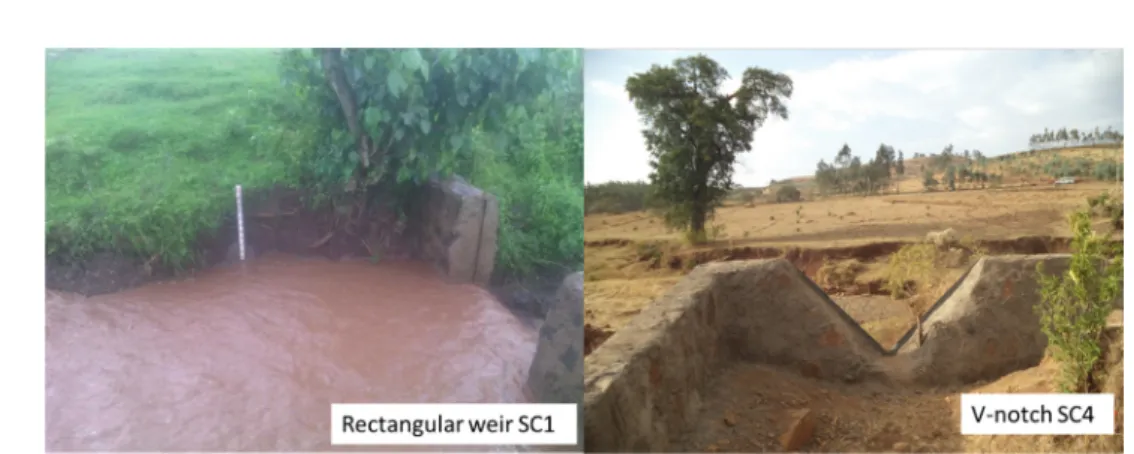
Hydrological monitoring stations were established at the outlet of every sub-catchment. The monitoring stations have a sharp- crested rectangular weir (in five catchments) and a V-notch weir at one sub-catchment (Fig. 3). During rainy seasons, the runoff stage was recorded every five minutes using a staff gauge and automatic pressure-transducer divers.
3.2. Determining runoff discharge from weirs
The discharge at the rectangular weirs was calculated as a function of the stage of the discharge (Aydin et al., 2011), using Eq.1–3:
Q = V(bh) (1) V = Cr√̅̅̅̅̅̅̅̅2gh (2) Cr = 0.153 ( b bmax )2 − 0.0922 ( b bmax ) +0.4136 (3)
where Q (m3 s−1) is the discharge, V (m s−1) is average runoff velocity, b (m) is the width of the opening of the weir, b
max (m) is the total
width of the weir, h (m) is the stage of the discharge, g (9.81 m s-2) is acceleration due to gravity, and Cr is a non-dimensional coefficient
for contracted weirs (b/bmax >0.3).
The discharge at the triangular weir was calculated from the stage height using Eq. 4 (Shen, 1981):
Q = 8 15xCvx ̅̅̅̅̅ 2g √ ×tan(θ 2 ) xh52 (4)
where Cv is the discharge coefficient (0.593 for a 90◦V-notch) and θ = 90 is the notch angle, in degrees.
3.3. Separating baseflow and quick flow
A runoff event (Q) was defined as the time between the start of rainfall and the end of the recession of quickflow (Fig. 4). Baseflow (Qb, mm) was separated from quickflow (Qqf, mm) using a function ‘BaseflowSeparation’ in the EcoHydrology package in R sofware
(Fuka et al., 2018), which uses a digital recursive filter algorithm (Gonzales et al., 2009; Nathan and McMahon, 1990). The analysis was performed using Eq. 5 and Eq. 6:
Qqf (t)= βQqf (t− 1)+ (1 + β) 2 [ Q(t)− Q(t− 1) ] (5)
Qb(t)= Q(t)− Qqf (t) (6)
It considers a filtering parameter (β) and the number of times of the application of the filter. We used β = 0.95 and a three pass filter (forward-backward-forward) (Liu et al., 2019; Zhang et al., 2013).
3.4. Defining catchment characteristics
A 30-m digital elevation model was obtained from the Shuttle Radar Topography Mission (http://www.earthexplorer.usgs.gov) to
Fig. 4. Example of event rainfall and runoff depth relation at sub-Catchment five (SC5) on 25th July 2018.
Table 1
Catchment characteristics of the study sub-catchments.
Sub-catchment
1 2 3 4 5 6
Catchment properties
Catchment area (A, ha) 82 53 68 20 47 44
Catchment length (D, m) 1353 1012 1281 759 1060 1032
Mean elevation (E, m a.s.l) 2445 2438 2379 2303 2329 2358
Mean slope (SG, %) 10.24 10.64 8.66 9.48 7.66 7.91
Steep slopes (SGs, % of SG > 10%) 44.2 41.7 28.5 43.2 21.9 24.2
Perimeter to area ratio (PA, m ha−1) 4.57 4.74 4.77 4.47 4.34 4.81
Distance to area ratio (DA, m ha−1) 1.51 1.41 1.56 1.7 1.56 1.57
GCI 1.29 1.34 1.35 1.23 1.23 1.36 TWI 6.34 6.55 6.61 6.46 6.68 6.78 Land Cover Forest (LCf, %) 37.8 1 0 15 4 2 Plantation (LCp %) 8.5 9 25 21 6 14 Shrub (LCs %) 2.4 26 4 0 5 0.5 Grazing (LCg %) 19.5 11 15 10 18 27.5 Cropland (LCc %) 28 49 54 52 65 54.5 Badland (LCb %) 1.4 4 1 0 0 0.5 Homestead (LCh %) 2.4 0 1 2 2 1 RFC (% cover) 13 12 18 22 21 18 NDVI 0.23 0.15 0.147 0.18 0.172 0.161 Soil properties
Average soil depth (SOILd, cm) 58 53 53 52 44 47
Sand content (SOILs, %) 57.29 53.2 49.59 54.5 54.65 59.38
Clay content (SOILc, %) 21.3 25.2 29.03 24.53 25.14 21.26
Organic matter content (SOILom, %) 5.2 3.1 2.7 3.1 3.6 3.8
Erosion and management
Gully density (Gd, m ha−1) 29.2 53.6 35.9 13.5 42.8 28.9
Bund density (Bd, m ha−1) 509 391 206 583 259 353
% area of steep slope vegetation (SSveg) 26.1 9.7 7.6 8.7 2.1 5
Stream properties
SPI 0.01 0.08 0.05 0.09 0.06 0.05
Note: m.a.s.l = meters above sea level, TWI = topographic wetness index, GCI = Gravel’s compactness index, SPI = stream power index, RFC = rock fragment cover (%), NDVI = normalised vegetation index.
delineate catchment boundaries and define catchment characteristics, including drainage area, slope gradient, catchment shape, and topographic indices (Table 1). The topographic wetness index (TWI = ln[A/tanβ]) and stream power index (SPI = A × tanβ) were determined using Q-GIS (A is the drainage area and β is the local slope angle in degrees). The corresponding Sentinel-2 satellite image was accessed from the Copernicus Open Access Hub (https://www.copernicus.eu), and land use/cover was classified in Q-GIS. Stone bund’s density and area of the badlands were mapped and estimated using Google Earth and Q-GIS (Fig. 1).
3.5. Curve number determination
The NRCS-CN model is an empirical model for estimating Qqf of ungauged catchments (Mishra and Singh, 2003; NRCS, 1997). It
uses a CN value that represents the hydrologic response of the area. The CN can be determined in two ways: i) from the standard NRCS table (NRCS, 1997); or ii) derived from measured P and Q data. This method assumes that the initial abstraction (Ia) is proportional to
the maximum potential retention (S, mm), which is expressed as Ia=λS where Ia is the initial abstraction, λ is the abstraction ratio and S is potential maximum retention (NRCS, 1997). Quickflow is then estimated from Eq. 7):
Qqf=
(P − λS)2
(P − λS + S) (7)
Valid for P ≥ λS, otherwise Qqf =0
The potential retention (S) is, however, not directly measured but derived from CN using Eq. 8:
S =25400
CN − 254 (8)
The use of the NRCS standard table considers land use, hydrologic soil group (HSG), and antecedent moisture condition (AMC) in determining CN values. The AMC was considered from the 5-day cumulative rainfall depth grouped into three classes: AMCI (< 36
mm), AMCII (36–53 mm), and AMCIII (> 53 mm) (Mishra and Singh, 2003). HSG was assigned based on soil texture class, bulk density,
and soil organic matter (SOILom). Hence, CN values were determined for each land use – HSG complex. The area-weighted average CN
was then determined for each sub-catchment (Eq. 9):
CNaω= ∑n i=1 ( CNx iAi ) ∑n i=1 Ai (9)
where CNaω is the area weighted CN, which is a median value (CNII) for the sub-catchment, Ai is the area for land use – HSG, and n is the
number of land use – HSG complexes.
CNII was then adjusted to slope (CNIIα) (Ajmal et al., 2020; Sharpley and Williams, 1990) (Eq. 10):
CNIIα= [ CNII(50 − 0.5CNII) CNII+75.43 ] × [ 1 – e − 7.125 (α– 0.05) ] + CNII (10)
CNI and CNIII are computed using the conversion formula given by (Hawkins et al., 1985).
CNI= CNII 2.281 − 0.001281CNII (11) CNIII= CNII 0.427 + 0.00573CNII (12)
The NRCS-CN, which was developed using λ = 0.2, was adjusted to equivalent CN for λ = 0.05 (Ajmal et al., 2020; Woodward et al., 2003b) (Eq. 13):
CN0.05=
100
1.42 − 0.0042 CN0.2 (13)
The second approach to curve number determination was based on measured rainfall–runoff datasets. For this, a non-linear least- squares function (nls), which uses the Gauss-Newton algorithm (Bates and Chambers, 1992) was used in R sofware, and the two parameters (λ and S) were determined, and the corresponding CN and Qqf were calculated using Eq. 8 and Eq. 7, respectively, for the
different AMCs. The least-squares fitting procedure generally takes the iteratively possible least square of residuals. Generally, CN is modelled for rainfall events exceeding 25 mm (Hawkins, 1993), but in this study, we considered events exceeding 10 mm because we found few events exceeding 25 mm.
CNs calculated from the rainfall–runoff data were compared with the tabulated NRCS-CN and analysed in relation to catchment
characteristics and management. The runoff prediction performance of the two methods (i.e. tabulated CN and rainfall-runoff data derived CN) was evaluated with the root mean square error (RMSE), Nash–Sutcliffe efficiency (NSE), percent bias (PBIAS), and co-efficient of determination (R2) (Moriasi et al., 2007).
3.6. Data analyses
Quickflow runoff coefficients (RCqf) were determined as the fraction of event Qqf to event P. Furthermore, lag-time (QL) for each
event was determined as the difference between the time to peak P and peak Qqf. ANOVA, correlation matrix, and principal component
analysis (PCA) were analysed using the R program for statistical computing (R Core Team, 2020) to relate quickflow to rainfall and catchment characteristics. When analysing multiple variables, the critical p-value (α) was adjusted (Bonferroni correction) to reduce
type I errors, which often increases with an increasing number of independent variables (Curtin and Schulz, 1998); otherwise, a significance level of α =0.05 was used.
4. Results
4.1. Spatial and temporal variability of rainfall
A total of n = 2348 rainfall–runoff events were analysed for all sub-catchments, occurring during the rainy seasons of three consecutive years. Sixty percent of the events had P < 5 mm. Average event P and I30 did not vary significantly among the sub-
catchments (p < 0.05). However, temporal variation was significant with P in June and I30 in August being higher than in other
months (Fig. 5 & Fig. 6). In addition, average event rainfall variability was significant across years.
4.2. Spatial and temporal variability of hydrological variables
Baseflow: Qb for the wet season starts in late June to early July, peaked in August, and declined gradually towards November
(Fig. 5). It was significantly higher in August than in other months (p < 0.01). The average baseflow coefficient (RCb) during rainfall-
runoff event was 7.3 %, while that of the seasonal RCb which also includes the baseflow between runoff events was 25 %.
Quickflow: There was significant variation in mean event Qqf among sub-catchments and years (p < 0.05) (Table 2, Fig. 6). The
average quickflow depth at SC6 was significantly lower than that at SC4. However, there was no significant difference in Qqf among the
remaining catchments. The average Qqf depth increased from June to August, when it was at its highest, and then declined until
October. The average RCqf across all catchments and years was 17 %.
Lag-time: QL varied significantly among the sub-catchments (p < 0.05). The average QL at SC3 was significantly lower than the
average QL at SC5 and SC6 (Table 2).
4.3. Relationship between rainfall and runoff variables
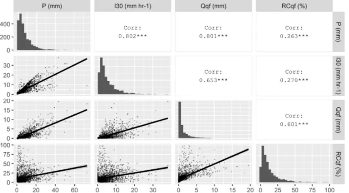
Event rainfall depth (P) and maximum 30-minute intensity (I30) had significant positive correlations (ɑ = 0.05) with quickflow
(Qqf) and the runoff coefficient (RCqf) (Fig. 7). The correlation between event quickflow and rainfall depth was strong and that between
quickflow and I30 was moderate (Fig. 7). The correlation between event rainfall and RCqf and between I30 and RCqf was also significant.
Analysis of variance among the three AMC groups revealed that there was a significant difference in the runoff coefficient as a function of antecedent moisture condition (ɑ = 0.01). Mean separation indicated that the runoff coefficient at AMCIII was significantly
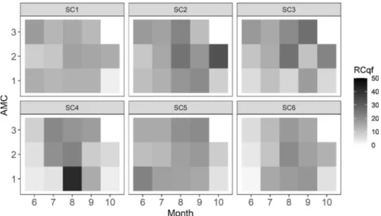
larger than that at AMCI and AMCII (Fig. 8). The seasonal distribution of runoff showed high runoff coefficients in August at AMCIII
(Fig. 9). During high antecedent moisture conditions, the rate of infiltration is low prompting an immediate generation of runoff. Hence, the high rate of quickflow during AMCIII, which was mostly in August, resulted in high runoff coefficient in August in general as
compared to other months. Besides, the spatial variability shows that the relationship between runoff response to antecedent moisture condition was minimized where forest cover was high (SC1). On the contrary, this relationship was more pronounced where cropland
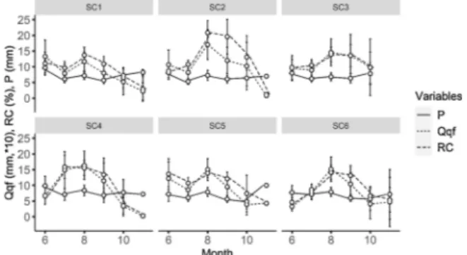
Fig. 5. Example of the variability of precipitation (P), quickflow (Qqf) and baseflow (Qb) throughout the rainy season (June - October 2018) at sub-
is dominant (SC3 and SC5) (Fig. 8). The variation in seasonal quickflow for different antecedent moisture conditions indicated that in the beginning of the rainy season (June) and at the end of the rainy season (October), the quickflow runoff coefficient response shows a clearly increasing trend from AMCI to AMCIII. However, in August, the quickflow coefficient response was high at all moisture
con-ditions. This could be due to increasing ground water table in the middle of the rainy season which increased the quickflow response regardless of the antecedent moisture condition.
4.4. Rainfall and catchment characteristics on the hydrological response
The rainfall variables such as P and I30 are strongly and positively correlated with runoff parameters particularly with quickflow
(Fig. 7). However, the correlation between P and I30 with the quickflow runoff coefficient was not strong.
The association of catchment characteristics with hydrological response variables of the sub-catchments is presented in a principal component biplot (Fig. 10). Principal component one (dim1) and principal component two (dim2) explain 53.1 % and 31 %, respectively, of the variability in the catchment characteristics and hydrological response of the catchments. Therefore, the two principal components explain 84 % of the variance, which is sufficient to consider the association to be strong. Accordingly, the hydrological response variables (Qqf, RCqf) are negatively associated with catchment area, forest, steep slopes with vegetation, soil
organic matter content and bund density (Fig. 10). On the other hand, crop land area (LCc) is positively associated with the
hydro-logical response variables. This clearly indicates the impact of land management and land cover characteristics to be prominent for catchment runoff response. Increasing vegetation cover, soil organic matter content and bund density reduces catchment quickflow and corresponding runoff coefficients. Whereas, increasing percent cropland area result in increasing runoff response.
4.5. Analysis of the curve number method for runoff prediction 4.5.1. CN values from NRCS-CN table and least square fitting methods
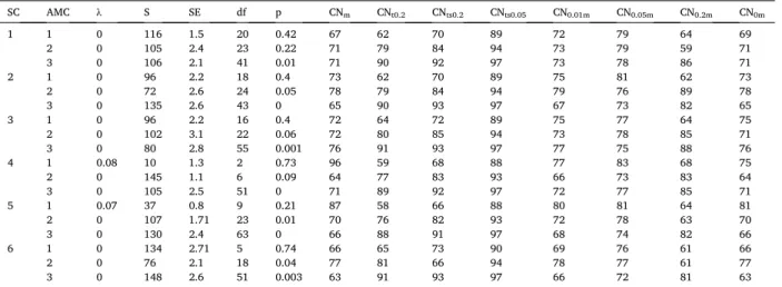
The CN from the NRCS-CN table of values ranged from 59 to 91, while the model-derived CN ranged from 63 to 96 (Table 3). The average abstraction ratio (λ) determined from the rainfall–runoff dataset was 0.05. However, the λ value for 88 % of the observations
Fig. 6. Variation of key hydrological parameters through time for the rainy seasons of 2018, 2019 and 2020. Qqf is 10 times exaggerated.
Table 2
Summary of event rainfall and runoff variables (mean ± standard deviation).
SC Year Qqf(mm) RCqf (%) QL(Minute) P (mm) I30 (mm h−1) n 1 2018 0.811 (0.1)) 7.3 (0.9) 45.8 (7.0) 10.8 (0.7) 6.94 (0.5) 59 2019 1.6 (0.2) 12.1 (1.2) 24.5 (2.6) 12 (0.7) 7.7 (0.6) 65 2020 2.86 (0.3) 20.9 (1.9) 28.8 (7.3) 12.9 (1.0) 7 (0.6) 61 2 2018 1.64 (0.2) 14 (0.9) 35.2 (4.9) 10.7 (0.7) 7 (0.5) 61 2019 1.29 (0.2) 9.1(0.6) 32.6 (3.3) 12.7 (0.8) 7.5 (0.6) 63 2020 4.52 (0.5) 32.2 (2.5) 31 (7.8) 14.4 (1.5) 7.2 (0.6) 57 3 2018 1.43 (0.3) 9 (1.0) 30.6 (3.8) 13.1 (1.0) 9.1 (0.7) 56 2019 2.95 (0.4) 19.6 (1.6) 25.1 (4.8) 13 (0.9) 8.3 (0.7) 69 2020 3.27 (0.4) 21.2 (1.9) 22.4 (8.6) 13.8 (1.3) 7 (0.6) 57 4 2018 1.96 (0.7) 18.5 (6.5) 82.8 (16.5) 12.1 (2.7) 7.3 (1.7) 9 2019 2.19 (0.3) 14.4 (1.4) 31.6 (4.9) 12.8 (0.8) 8.9 (0.6) 74 2020 3.48 (0.5) 23.4 (2.1) 45.5 (11.6) 14.9 (1.9) 8.3(1.0) 33 5 2018 2.17 (0.3) 16.5 (1.1) 28.5 (4.0) 11.7 (1.0) 7.9 (0.6) 66 2019 2.3 (0.2) 16.8 (1.0) 31.2 (3.6) 12.3 (0.8) 8.1 (0.6) 82 2020 2.47 (0.3) 16.6 (1.5) 75.6 (21.1) 14 (1.5) 7.5 (0.7) 52 6 2018 1.72 (0.3) 12.5 (1.3) 34.8 (3.2) 11.3 (0.8) 7.5 (0.6) 63 2019 1.76 (0.2) 13.1 (1.0) 29.8 (3.7) 11.9 (0.7) 7.8 (0.5) 81 2020 2.44 (0.4) 18.6 (2.8) 59 (14.8) 14.3 (1.7) 8.1 (0.9) 39
was zero.
4.5.2. Model performance analysis
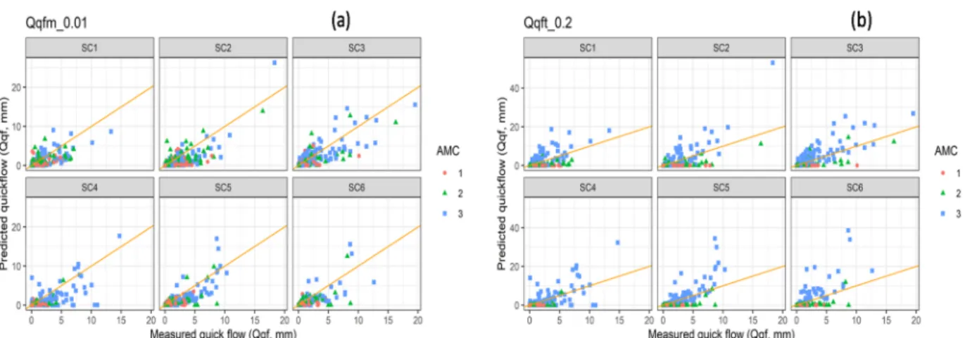
The CN fitted to the rainfall-runoff dataset demonstrated that it was best fitted at λ = 0.01 and λ = 0, explaining approximately 57–69 % of the variability in the quickflow response (Fig. 11). However, the data fitted at λ = 0.2 could explain only 49–63 % of the quickflow response. The table CN prediction also confirmed that the capability of the NRCS-CN model was less satisfactory at λ = 0.2 (Table 4). The NRCS-CN model performance was relatively good for λ = 0.05 and 0.01, explaining 56–76 % of the variability in the quickflow response. The data-based models at λ = 0.01 and λ = 0 produced comparable results. Compared to the other models, λ =
Fig. 7. Correlation matrix of the variables I30 (30-minute maximum intensity), P (event rainfall depth in mm), Qqf (event quickflow depth in mm),
and RCqf (event runoff coefficient in %).
Fig. 8. Quick flow runoff coefficient (RC in %) at different antecedent moisture conditions expressed as five day cumulative rainfall depth: AMC I <
0.01 and λ = 0 performed well, with NSE values ranging from 0.51 to 0.64 (Table 4). This implies that λ values ≤ 0.01 improve the prediction efficiency. In general, the data-based NRCS-CN model performance for λ = 0.01 and λ = 0 showed relatively satisfactory performance for most of the evaluation criteria (Moriasi et al., 2007).
Fig. 9. Average runoff coefficient (RC in %) values for the 6 sub-catchments in the different months and antecedent moisture conditions (AMC,
expressed by five-day cumulative rainfall depth classes; 1 for cumulative rainfall ≤ 36 mm, 2 for 53 mm < cumulative rainfall ≤ 53 mm, and 3 for cumulative rainfall > 53 mm).
Fig. 10. Principal component biplot (PCA) for the catchment characteristics and runoff; Dim1 is principal component one and dim2 is principal
component two (the variables LCh, LCb, LCf, LCc, LCs stands for homestead, badlands, forest, cropland and shrub land covers; DA is catchment distance to area ratio, RF is rainfall, RFC is rock fragment cover, Q is total flow discharge, qf is quickflow, bf is baseflow, RC is runoff coefficient, SOILom is soil organic matter, SSveg is steep slope vegetation, CA is catchment area, Bd is stone bund density, E is elevation, Gd is Gravelel’s shape index).
5. Discussion
5.1. Effect of rainfall variables on the runoff response
Quickflow was positively correlated with rainfall depth and intensity, but the runoff coefficient (RC) was not significant. This can be due to the effect of the antecedent moisture condition (AMC), which had a significant effect on the RC. This indicates that runoff was mostly of the saturation excess type, rather than the infiltration excess type. Hence, during high values of AMC, RC was large irre-spective of rainfall depth. Similarly, Steenhuis et al. (2009) reported that the runoff generation mechanism is mostly saturation excess in the Lake Tana Basin. The higher quickflow in August is also associated with low surface roughness as a result of smoothing due to local erosion and deposition as well as raindrop impact of the prior rainfall events. Whereas, the land management activities in June, particularly plowing, increases the surface roughness and enhances infiltration resulting in low quickflow. The higher baseflow in August can be attributed to the frequent rains. Besides, the ground water table normally rises during August, which could contribute to the peak baseflow.
5.2. The performance of the CN method for runoff prediction
The NRCS-CN set λ = 0.2 in its initial publication. However, this was found to be too high and a new value of λ = 0.05 was reported as an improved standard (Descheemaeker et al., 2008; Savvidou et al., 2018; Woodward et al., 2003a). The NRCS-CN was developed for gentle slopes of approximately 5% (Savvidou et al., 2018). In addition, the NRCS-CN model predicts CN values that are too large for small rainfall events (Woodward et al., 2003b). From the least square fitting approach, we found a much lower value, close to zero, and λ =0.01 was found to be appropriate for the study area. This low abstraction ratio implies that the initial abstraction is only a small fraction of the potential retention. This may be related to the AMC, which was relatively larger in our sub-humid study area than in
Table 3
Summary of rainfall-runoff database curve number for sub-catchments at different AMC.
SC AMC λ S SE df p CNm CNt0.2 CNts0.2 CNts0.05 CN0.01m CN0.05m CN0.2m CN0m 1 1 0 116 1.5 20 0.42 67 62 70 89 72 79 64 69 2 0 105 2.4 23 0.22 71 79 84 94 73 79 59 71 3 0 106 2.1 41 0.01 71 90 92 97 73 78 86 71 2 1 0 96 2.2 18 0.4 73 62 70 89 75 81 62 73 2 0 72 2.6 24 0.05 78 79 84 94 79 76 89 78 3 0 135 2.6 43 0 65 90 93 97 67 73 82 65 3 1 0 96 2.2 16 0.4 72 64 72 89 75 77 64 75 2 0 102 3.1 22 0.06 72 80 85 94 73 78 85 71 3 0 80 2.8 55 0.001 76 91 93 97 77 75 88 76 4 1 0.08 10 1.3 2 0.73 96 59 68 88 77 83 68 75 2 0 145 1.1 6 0.09 64 77 83 93 66 73 83 64 3 0 105 2.5 51 0 71 89 92 97 72 77 85 71 5 1 0.07 37 0.8 9 0.21 87 58 66 88 80 81 64 81 2 0 107 1.71 23 0.01 70 76 82 93 72 78 63 70 3 0 130 2.4 63 0 66 88 91 97 68 74 82 66 6 1 0 134 2.71 5 0.74 66 65 73 90 69 76 61 66 2 0 76 2.1 18 0.04 77 81 66 94 78 77 61 77 3 0 148 2.6 51 0.003 63 91 93 97 66 72 81 63
Note: λ = abstraction coefficient; S = retention parameter; SE = standard error; df = degree of freedom; CNm =curve number derived from the measured P and Qqf; CNt0.2 is NRCS-table curve number at λ = 0.2; CNts0.2 is CNt0.2 adjusted for slope; CNts0.05 is CNts0.2 converted for λ = 0.05, and
CN0.01m, CN0.05m, CN0.2m and CN0m are curve numbers from the measured P and Qqf data at λ = 0.01, λ = 0.05, λ = 0.2 and λ = 0, respectively.
Fig. 11. Event rainfall depth (P) and corresponding quickflow runoff depth (Qqf) for three antecedent moisture conditions fitted to different λ values
semi-arid locations, where a λ value of 0.05 was more appropriate (Descheemaeker et al., 2008; Fu, 2016). Therefore, determining the most appropriate λ values in sub-humid locations, where the soil is mostly saturated, requires further investigation. Examination of the performance using different λ values indicated that λ = 0.01 and λ = 0 were significant in most cases considered (Table 4).
The runoff prediction using NRCS-table CN overestimated the quickflow (Fig. 12b), while the data derived models underestimate it (Fig. 12a). In addition, the distribution of data along the l:1 line exhibits considerably higher variability. This implies that the applicability of the CN method for runoff prediction needs further consideration, including improvement of the abstraction ratio and reconsideration of the range of the AMC when grouping AMC into three categories. One of the limitations of the use of the CN method is its consideration of only high rainfall events (> 25 mm), which represent only a small fraction of the total rainfall events, even in the heavy rainy seasons in the present study.
Table 4
The Quickflow (Qqf) prediction performance of the different models considered.
SC Criteria NRCS-table P and Qqf Data based
λ =0.2 λ =0.05 λ =0.01 λ =0.05 λ =0.2 λ =0 1 PBIAS % 31.6 172.4 − 33.2 − 49.8 −72.6 −28.9 RSR 1.69 2.27 0.7* 0.78 0.96 0.68* NSE −1.86 −4.15 0.51* 0.4 0.08 0.54* R2 0.52* 0.64** 0.56* 0.5* 0.31 0.57* 2 PBIAS % −24.9* 95.6 − 39.8 − 56.3 −67.1 −36.2 RSR 1.24 1.68 0.68* 0.76 0.86 0.66* NSE −0.54 −1.84 0.54* 0.43 0.25 0.57* R2 0.49 0.65** 0.61* 0.54* 0.48 0.62* 3 PBIAS % 0.2*** −123.8 − 22.4* − 47.7 −46.4 18* RSR 0.94 1.5 0.58** 0.65* 0.7* 0.58** NSE 0.12 −1.25 0.66** 0.57* 0.52* 0.67** R2 0.62* 0.69** 0.68** 0.63* 0.6* 0.68** 4 PBIAS % 6.5*** 107.4 − 33.7 − 41.4 −54.9 −30.4 RSR 1.16 1.74 0.64* 0.69* 0.81 0.62* NSE −0.35 −2.04 0.59* 0.52* 0.35 0.61* R2 0.63* 0.69** 0.65** 0.62* 0.54* 0.66** 5 PBIAS % −12.3** 105.6 − 37.2 − 48 −73 −32.3 RSR 1.31 1.92 0.63* 0.71 0.94 0.6** NSE −0.73 −2.68 0.61* 0.49 0.11 0.64V R2 0.59* 0.76*** 0.68** 0.62* 0.4 0.69** 6 PBIAS % 31.6 172.4 − 33.2 − 49.8 −72.6 −28.9 RSR 1.69 2.27 0.7* 0.78 0.96 0.68* NSE −1.86 −4.15 0.51* 0.4 0.08 0.54* R2 0.52* 0.64* 0.56* 0.5* 0.31 0.57*
*=satisfactory, Qt_0.2, Qt_0.05 = runoff predicted based on NRCS-Table CN at λ = 0.2 and 0.05 respectively; Qp_0.01, Qp_0.05, Qp_0.2 and Qp_0
are runoff predicted based on CN model from rainfall-runoff dataset for λ = 0.01, λ = 0.05, λ = 0.2 and λ = 0 respectively.
**=good.
***=indicates very good.
Fig. 12. Predicted quickflow (Qqf, mm) using data-derived CN at λ = 0.01 (a), Predicted quickflow (Qqf, mm) using NRCS-table CN at λ = 0.2 (b).
5.3. Rainfall and catchment characteristics that affect the runoff response
The depth of rainfall alone could explain approximately 60 % of the variability in quickflow response, but could only explain approximately 5% of the variability in the runoff coefficient. This indicates that the runoff coefficient is a more complex variable that could be more strongly influenced by catchment characteristics.
Runoff was negatively associated with vegetation cover, stone bund density and average soil organic matter content. Most of the forest and shrubs were located on steep slopes (Fig. 2). This would have enhanced water retention through interception, improved infiltration, and reduced overland flow depth.
Runoff responses vary among land uses (Descheemaeker et al., 2008; Sultan et al., 2017). Rehabilitating degraded areas through exclosures reduced runoff significantly, making vegetation cover the primary variable explaining differences in runoff generation. Increasing vegetation was also associated with reducing runoff curve numbers from rehabilitating lands in semi-arid areas (Descheemaeker et al., 2008). Bayabil et al. (2010) demonstrated that runoff from gentle sloping cropland areas was higher than for grasslands and woodlands on steeper plots. Rehabilitating runoff source areas, including degraded steep slopes and grazing areas, plays a vital role in reducing catchment runoff. The results of this study are also in agreement with those studies.
The topographic position also exerts an influence on runoff mechanisms. It explains the type of runoff in the area, which is characterised by saturation excess, particularly during the main rainy season (Akale et al., 2017; Steenhuis et al., 2009; Tilahun et al., 2016), due to the presence of a hardpan (Hussein et al., 2019) or rapidly rising shallow groundwater tables. Hence, upslope steep areas are less likely to be saturated from rising water tables and they drain soil moisture quickly through sub-surface flows. Therefore, the generation of runoff in steep slopes can be relatively slow during the wet season compared to the mostly saturated low-lying gentle slopes. Dessie et al. (2014) in the Lake Tana Basin, and Taye et al. (2013) in northern Ethiopia, also demonstrated that runoff decreased with increasing areas of steep slopes. In northern Ethiopia, this trend was explained by an increased rock fragment cover with increasing slope gradient, resulting in larger infiltration rates on steep slopes (Taye et al., 2013). A subject of great concern related to the efficient drainage of steep upland slopes versus high runoff generation on gentle valley floor slopes is the development of valley floor gullies, especially since intensive soil and water conservation efforts are not paying off in terms of gully control (Frankl et al., 2021). Valley floor vegetation in runoff concentration zones has been suggested as a measure to increase the resistance of soil to gully development (Frankl et al., 2019).
Stone bunds are important land management practices that are widely practiced in cultivated landscapes of sub-Sahara Africa (Wolka et al., 2018) and the highlands of Ethiopia in particular (Nyssen et al., 2015; Vancampenhout et al., 2006). In Ethiopia, soil and water conservation practices have significantly reduced soil erosion and improved soil moisture retention and agricultural produc-tivity (Akale et al., 2017; Jemberu et al., 2018; Vancampenhout et al., 2006; Wolka et al., 2011). In general multitude of catchment characteristics of both natural and anthropogenic factors affect the runoff mechanism in an intertwined manner. Hence, the land management in the area should take into account of the role of vegetation and stone bunds in steep slope areas and practices that enhance soil organic matter in cropland areas.
6. Conclusions
This study demonstrated that runoff in the studied catchments was strongly correlated to rainfall characteristics and antecedent soil moisture content. The runoff mechanism in the area was found to be mostly of saturation excess. The average runoff coefficient of quickflow was only 17 %. This low value is mainly attributed to the role of recent land management activities intensively implemented in the area, particularly the installation of stone bunds and vegetation rehabilitation. However, quickflow exhibited significant variability in space and time. Catchment runoff is a complex process affected by a multitude of catchment characteristics, including catchment shape parameters, topography, vegetation cover, management and soil properties. In particular, vegetation cover, stone bunds and soil organic matter are negatively associated with quickflow, underlining the role of management on runoff production. Hence, measures that enhance the infiltration capacity of the soil and modify local topography are of paramount importance in land management. In this regard, stone bunds and especially vegetation rehabilitation in steep slope areas should be encouraged, especially in runoff concentration zones susceptible to gullying. The available NRCS-CN table values were found to overestimate the predicted runoff, and to show a wide scatter around the 1:1 line. This is because the model was developed based on large rainfall events yet often used to predict event runoff from small rainfall depths. Hence, there is a need to optimize the model to make it more appropriate for areas where event rainfall is low but frequent. An important finding of this study was that the abstraction ratio (λ) for use in the NRCS-
CN model for runoff prediction was optimal at 0.01, rather than the usually recommended 0.05 or 0.2 used in hydrological modelling
programs such as SWAT. Unless a locally optimised λ is used, we recommend application of our value in similar agroecological areas.
Author statement
Amaury Frankl, Jan Nyssen, Jean Poesen, Enyew Adgo, Derege Tsegaye Meshesha and Alemayehu Wassie were involved in the conceptualization of the project. Habtamu Assaye, Amaury Frankl and Alemayehu Wassie selected the study site. Habtamu Assaye and Amaury Frankl developed the methodology. Habtamu Assaye installed hydro-meteorological stations, collected and analyzed the data and prepared the original draft manuscript. Amaury Frankl, Jan Nyssen, Jean Poesen and Hanibal Lemma contributed on the improvement of the manuscript. All authors had visited the research site repeatedly. Amaury Frankl, Jan Nyssen, Enyew Adgo and Alemayehu Wassie were involved in the management of the project.
Declaration of Competing Interest
This is to confirm that there is no conflict of interest among the authors. I am the corresponding author and am responsible for any communication concerning the publication of this manuscript.
Acknowledgments
The authors acknowledge the financial support provided by the VLIR-UOS through the Institutional University Cooperation (IUC) project of Bahir Dar University, Ethiopia and Ghent University, Belgium. We are grateful to the BDU-IUC office staff for smoothly facilitating financial and purchase-related activities. We are particularly thankful to Derbew Fente, who supported the project immensely during the field installation and monitoring activities. Banchigize Habesha, Amsalu Akanaw, and Getachew Dagne are also acknowledged for their unwavering support. Tadla Girmay is acknowledged for her support in laboratory activities. Akanaw Abebaw, an expert at Dera Woreda Agriculture and Natural Resources Department; Marelign Tigabu and Fente Yihune local development agents at Gelawdiwos and Shime Kebeles, respectively, are acknowledged for facilitating the initial activities of the project and organising data collectors. Melese Geze, Alelign Gardew, and Gebreegziabher Fentahun (MSs-students involved during data collection) are also acknowledged. Last, but most importantly, local data collectors are acknowledged for their crucial support and keenness.
Appendix A. Supplementary data
Supplementary material related to this article can be found, in the online version, at doi:https://doi.org/10.1016/j.ejrh.2021. 100819.
References
Abate, M., Nyssen, J., Steenhuis, T.S., Moges, M.M., Tilahun, S.A., Enku, T., Adgo, E., 2015. Morphological changes of Gumara River channel over 50 years, Upper Blue Nile Basin, Ethiopia. J. Hydrol. 525, 152–164. https://doi.org/10.1016/j.jhydrol.2015.03.044.
Adem, A.A., Aynalem, D.W., Tilahun, S.A., Steenhuis, T.S., 2017. Predicting reference evaporation for the Ethiopian highlands. J. Water Resour. Prot. 09, 1244–1269.
https://doi.org/10.4236/jwarp.2017.911081.
Ajmal, M., Waseem, M., Kim, D., Kim, T.W., 2020. A pragmatic slope-adjusted curve number model to reduce uncertainty in predicting flood Runo ff from steep watersheds. Water (Switzerland) 12. https://doi.org/10.3390/w12051469.
Akale, A.T., Id, D.C.D., Belete, M.A., Tilahun, S.A., Mekuria, W., Steenhuis, T.S., 2017. Impact of Soil Depth and Topography on the Effectiveness of Conservation Practices on Discharge and Soil Loss in the Ethiopian Highlands. n.d.. https://doi.org/10.3390/land6040078.
Aydin, I., Altan-Sakarya, A.B., Sisman, C., 2011. Discharge formula for rectangular sharp-crested weirs. Flow Meas. Instrum. 22, 144–151. https://doi.org/10.1016/j. flowmeasinst.2011.01.003.
Bates, D.M., Chambers, J.M., 1992. Nonlinear models. In: Chambers, J.M., Hastie, T.J. (Eds.), Statistical Models in S. Routledge, NY, pp. 421–453.
Bayabil, H.K., Tilahun, S.A., Collick, A.S., Yitaferu, B., Steenhuis, T.S., 2010. Are runoff processes ecologically or topographically driven in the (sub) humid Ethiopian highlands? The case of the Maybar watershed. Ecohydrology 3, 457–466.
Boardman, J., 2018. The value of Google Earth TM for erosion mapping. Catena 143, 123–127. https://doi.org/10.1016/j.catena.2016.03.031.
Bruin, D., Karlberg, L., Hoff, H., Andersson, K., Binnington, T., Flores-l´opez, F., Gebrehiwot, S.G., Johnson, O., Osbeck, M., Young, C., 2015. Tackling complexity: understanding the food-energy-environment Nexus in Ethiopia’s Lake Tana sub-basin. Water Altern. 8, 710–734.
Colot, C., 2012. Soil-landscape Relation at Regional Scale in Lake Tana basin (Ethiopia). MSc Thesis. Faculteit Bio-ingenieurswetenschappen, KU Leuven. Curtin, F., Schulz, P., 1998. Multiple correlations and Bonferroni’s correction. Biol. Psychiatry. https://doi.org/10.1016/S0006-3223(98)00043-2.
de Vente, J., Poesen, J., 2005. Predicting soil erosion and sediment yield at the basin scale: scale issues and semi-quantitative models. Earth-Sci. Rev. 71, 95–125. Descheemaeker, K., Poesen, J., Borselli, L., Nyssen, J., Raes, D., Haile, M., Muys, B., Deckers, J., 2008. Runoff curve numbers for steep hillslopes with natural
vegetation in semi-arid tropical highlands, northern Ethiopia. Hydrol. Process 4105, 4097–4105. https://doi.org/10.1002/hyp.
Dessie, M., Verhoest, N.E.C., Pauwels, V.R.N., Admasu, T., Poesen, J., Adgo, E., Deckers, J., Nyssen, J., 2014. Analyzing runoff processes through conceptual hydrological modeling in the Upper Blue Nile Basin, Ethiopia. Hydrol. Earth Syst. Sci. 18, 5149–5167. https://doi.org/10.5194/hess-18-5149-2014.
Ebabu, K., Tsunekawa, A., Haregeweyn, N., Adgo, E., Meshesha, D.T., Aklog, D., Masunaga, T., Tsubo, M., Sultan, D., Fenta, A.A., Yibeltal, M., 2019. Effects of land use and sustainable land management practices on runoff and soil loss in the Upper Blue Nile basin, Ethiopia. Sci. Total Environ. 648, 1462–1475.
FDRE, 2011. Ethiopia’s Climate-resilient Green Economy: Green Economy Strategy. The Government of the Federal Democratic Republic of Ethiopia (FDRE), Addis Ababa, Ethiopia.
Frankl, A., Nyssen, J., Adgo, E., Wassie, A., Scull, P., 2019. Can woody vegetation in valley bottoms protect from gully erosion? Insights using remote sensing data (1938–2016) from subhumid NW Ethiopia. Reg. Environ. Chang. 19, 2055–2068. https://doi.org/10.1007/s10113-019-01533-4.
Frankl, A., Nyssen, J., Vanmaercke, M., Poesen, J., 2021. Gully prevention and control: techniques, failures and effectiveness. Earth Surf. Process. Landforms 46, 220–238. https://doi.org/10.1002/esp.5033.
Fu, S., 2016. Initial Abstraction Ratio in the SCS-CN Method in the Loess Plateau of China. https://doi.org/10.13031/2013.36271.
Fuka, D.R., Walter, M.T., Archibald, J.A., Steenhuis, T.S., Easton, Z.M., 2018. EcoHydRology: A Community Modeling Foundation for Eco-hydrology.
Gebresellassie, Z.D., 2017. Spatial mapping and testing the applicability of the curve number method for ungauged catchments in Northern Ethiopia. Int. Soil Water Conserv. Res. 5, 293–301. https://doi.org/10.1016/j.iswcr.2017.06.003.
Gonzales, A.L., Nonner, J., Heijkers, J., Uhlenbrook, S., 2009. Comparison of different base flow separation methods in a lowland catchment. Hydrol. Earth Syst. Sci. 13, 2055–2068. https://doi.org/10.5194/hess-13-2055-2009.
Guzha, A.C., 2018. Impacts of land use and land cover change on surface runo ff, discharge and low flows: evidence from East Africa. J. Hydrol. Reg. Stud. 15, 49–67.
https://doi.org/10.1016/j.ejrh.2017.11.005.
Hawkins, R.H., 1993. Asymptotic determination of runoff curve numbers from data. J. Irrig. Drain. Eng. 119, 334–345. https://doi.org/10.1061/(ASCE)0733-9437 (1993)119:2(334).
Hawkins, R.H., Hjelmfelt, A.T., Zevenbergen, A.W., 1985. Runoff probability, storm depth, and curve numbers. J. Irrig. Drain. Eng. 111, 330–340. https://doi.org/ 10.1061/(ASCE)0733-9437(1985)111:4(330).
Heckmann, T., Cavalli, M., Cerdan, O., Foerster, S., Javaux, M., Lode, E., Smetanov´a, A., Vericat, D., Brardinoni, F., 2018. Indices of sediment connectivity: opportunities, challenges and limitations. Earth-Science Rev. 187, 77–108. https://doi.org/10.1016/j.earscirev.2018.08.004.
Hussein, M.A., Muche, H., Schmitter, P., Nakawuka, P., Tilahun, S.A., Langan, S., Barron, J., Steenhuis, T.S., 2019. Deep tillage improves degraded soils in the (Sub) Humid Ethiopian Highlands. Land 8. https://doi.org/10.3390/land8110159.
Jemberu, W., Baartman, J.E.M., Fleskens, L., Ritsema, C.J., 2018. Participatory assessment of soil erosion severity and performance of mitigation measures using stakeholder workshops in Koga catchment, Ethiopia. J. Environ. Manage. 207, 230–242. https://doi.org/10.1016/j.jenvman.2017.11.044.
Johansson, B., 1994. The relationship between catchment characteristics and the parameters of a conceptual runoff model: a study in the south of Sweden. In: Seuna, P., Gustard, A., Arnell, N.W., Cole, G.A. (Eds.), FRIEND: Flow Regimes from International Experimental and Network Data. IAHS Pub. No. 221, Wallingford, UK, pp. 475–482.
Kamuju, N., 2015. Sensitivity of initial abstraction coefficient on prediction of rainfall- runoff for various land cover classes of ‘ton watershed’ using remote sensing & GIS based ‘rinspe’ model. IJSRST 1, 213–221.
Karamage, F., Zhang, C., Fang, X., Liu, T., Ndayisaba, F., Nahayo, L., Kayiranga, A., Nsengiyumva, J.B., 2017. Modeling rainfall-runoffresponse to land use and land cover change in Rwanda (1990-2016). Water (Switzerland) 9. https://doi.org/10.3390/w9020147.
Lemann, T., Roth, V., Zeleke, G., Subhatu, A., Kassawmar, T., Hurni, H., 2019. Spatial and Temporal Variability in Hydrological Responses of the Upper Blue Nile Basin, Ethiopia. https://doi.org/10.3390/w11010021.
Lemma, H., Admasu, T., Dessie, M., Fentie, D., Deckers, J., Frankl, A., Poesen, J., Adgo, E., Nyssen, J., 2018. Revisiting lake sediment budgets: how the calculation of lake lifetime is strongly data and method dependent. Earth Surf. Process. Landforms 43, 593–607.
Lemma, H., Frankl, A., van Griensven, A., Poesen, J., Adgo, E., Nyssen, J., 2019a. Identifying erosion hotspots in Lake Tana basin from a multisite soil and water assessment tool validation: opportunity for land managers. L. Degrad. Dev. 30, 1449–1467.
Lemma, Hanibal, Frankl, A., van Griensven, A., Poesen, J., Adgo, E., Nyssen, J., 2019b. Identifying erosion hotspots in Lake Tana basin from a multisite soil and water assessment tool validation: opportunity for land managers. L. Degrad. Dev. 30, 1449–1467. https://doi.org/10.1002/ldr.3332.
Liu, Z., Liu, S., Ye, J., Sheng, F., You, K., Xiong, X., 2019. Application of a Digital Filter Method to Separate Baseflow in the Small Watershed of Pengchongjian in.
Minale, A.S., 2013. Population and environment interaction : the case of gilgel abbay catchment, northwestern Ethiopia. E3 J. Environ. Res. Manag. 4, 153–162.
Mishra, S.K., Singh, V.P., 2003. Soil Conservation Cervice Curve Number (SCS-CN) Methodology. Springe, Netherlands.
MoFED, 2010. Growth and Transformation Plan I (GTP I): 2011-2015. Ethiopian Ministry of Finance and Economic Development (MoFED), Addis Ababa. Monsieurs, E., Poesen, J., Dessie, M., Adgo, E., Verhoest, N.E.C., Deckers, J., Nyssen, J., 2015. Effects of drainage ditches and stone bunds on topographical thresholds
for gully head development in North Ethiopia. Geomorphology 234, 193–203. https://doi.org/10.1016/j.geomorph.2015.01.011.
Moriasi, D.N., Arnold, J.G., van Liew, M.W., Bingner, R.L., Harmel, R.D., Veith, T.L., 2007. Model evaluation guidelines for systematic quantification of accuracy in watershed simulations. Trans. ASABE 50, 885–900.
Nathan, R.J., McMahon, T.A., 1990. Evaluation of automated techniques for base flow and recession analyses. Water Resour. Res. 26, 1465–1473. https://doi.org/ 10.1029/WR026i007p01465.
NPC, 2015. Growth and Transformation Plan II (GTP II): 2015-2020. National Planning Commission (NPC), Addis Ababa, Ethiopia.
NRCS, 1997. National Engineering Handbook (Section 4, Hydrology). Natural Resources Conservation Service (NRCS), US Department of Agriculture, Washington, DC.
Nyssen, J., Poesen, J., Lanckriet, S., Jacob, M., Moeyersons, J., Haile, M., Haregeweyn, N., Munro, R.N., Descheemaeker, K., Adgo, E., Frankl, A., Deckers, J., 2015. Land degradation in the Ethiopian highlands. In: Billi, P. (Ed.), Landscapes and Landforms of Ethiopia. Springer, The Netherlands, pp. 369–385.
Peel, M.C., Finlayson, B.L., Mcmahon, T.A., 2007. Updated world map of the K¨oppen-Geiger climate classification. Hydrol. Earth Syst. Sci. Discuss.
Pilgrim, D.H., Cordery, I., Baron, B.C., 1982. Effects of catchment size on runoff relationships. J. Hydrol. Poesen, J., 2018. Soil erosion in the Anthropocene: research needs. Earth Surf. Process. Landforms 43, 64–84.
Poppe, L., Frankl, A., Poesen, J., Admasu, T., Dessie, M., Adgo, E., Deckers, J., Nyssen, J., 2013. Geomorphology of the Lake Tana Basin, Ethiopia. J. Maps 9, 431–437.
R Core Team, 2020. R: a Language and Environment for Statistical Computing.
Rodríguez-Blanco, M.L., Taboada-Castro, M.M., Taboada-Castro, M.T., 2012. R´eponse pluie-d´ebit et coefficients de ruissellement ´ev´enementiels dans une r´egion humide (nordouest de l’Espagne). Hydrol. Sci. J. 57, 445–459. https://doi.org/10.1080/02626667.2012.666351.
Savvidou, E., Efstratiadis, A., Koussis, A.D., Koukouvinos, A., Skarlatos, D., 2018. The curve number concept as a driver for delineating hydrological response units. Water (Switzerland) 10. https://doi.org/10.3390/w10020194.
Setegn, S.G., Srinivasan, R., Dargahi, B., Melesse, A.M., 2009. Spatial delineation of soil erosion vulnerability in the Lake Tana Basin, Ethiopia. Hydrol. Process. 23, 3738–3750.
Sharpley N, Andrew, Williams, 1990. EPIC, Erosion/Productivity Impact Calculator. 1, Model documentation. U.S. Dept. of Agriculture, Agricultural Research Service, Washington, D.C.
Shen, J., 1981. Discharge characteristics of triangular-notch thin-plate weirs. Geol. Surv. Water-Supply Pap. 1617-B, p. 62.
Sitterson, J., Knightes, C., Parmar, R., Wolfe, K., Muche, M., Avant, B., 2017. An overview of rainfall-runoff model types. U.S. Environ. Prot. Agency 0–29. Steenhuis, T.S., Collick, A.S., Easton, Z.M., Leggesse, E.S., Bayabil, H.K., White, E.D., Awulachew, S.B., Adgo, E., Ahmed, A.A., 2009. Predicting discharge and
sediment for the Abay (Blue Nile) with a simple model. Hydrol. Process. 23, 3728–3737. https://doi.org/10.1002/hyp.7513.
Sultan, D., Tsunekawa, A., Haregeweyn, N., Adgo, E., Tsubo, M., Meshesha, D.T., Masunaga, T., Aklog, D., Ebabu, K., 2017. Analyzing the runoff response to soil and water conservation measures in a tropical humid Ethiopian highland. Phys. Geogr. 38, 423–447.
Taye, G., Poesen, J., Wesemael, B.V., Vanmaercke, M., Teka, D., Deckers, J., Goosse, T., Maetens, W., Nyssen, J., Hallet, V., Haregeweyn, N., 2013. Effects of land use, slope gradient, and soil and water conservation structures on runoff and soil loss in semi-arid Northern Ethiopia. Phys. Geogr. 34, 236–259.
Temesgen, G., Amare, B., Abraham, M., 2014. Population dynamics and land use/land cover changes in Dera District, Ethiopia. Glob. J. Biol. Agric. Heal. Sci. 3, 134–140.
Tilahun, S.A., Ayana, E.K., Guzman, C.D., Dagnew, D.C., Zegeye, A.D., Tebebu, T.Y., Yitaferu, B., Steenhuis, T.S., 2016. Revisiting storm runoff processes in the upper Blue Nile basin: the Debre Mawi watershed. Catena 143, 47–56. https://doi.org/10.1016/j.catena.2016.03.029.
Vancampenhout, K., Nyssen, J., Gebremichael, D., Deckers, J., Poesen, J., Haile, M., Moeyersonse, J., 2006. Stone bunds for soil conservation in the northern Ethiopian highlands: impacts on soil fertility and crop yield. Soil Tillage Res. 90, 1–15.
Vanmaercke, Matthias, Poesen, J., Broeckx, J., Nyssen, J., 2014a. Earth-science reviews sediment yield in Africa. Earth Sci. Rev. 136, 350–368. https://doi.org/ 10.1016/j.earscirev.2014.06.004.
Vanmaercke, M., Poesen, J., Broeckx, J., Nyssen, J., 2014b. Sediment yield in Africa. Earth Sci. Rev. 136, 350–368. https://doi.org/10.1016/j.earscirev.2014.06.004. Wolka, K., Moges, A., Yimer, F., 2011. Effects of Level Soil Bunds and Stone Bunds on Soil Properties and its Implications for Crop Production: the Case of Bokole
Watershed, Dawuro Zone, Southern Ethiopia. https://doi.org/10.4236/as.2011.23047.
Wolka, K., Mulder, J., Biazin, B., 2018. Effects of soil and water conservation techniques on crop yield, runoff and soil loss in Sub-Saharan Africa: a review. Agric. Water Manag. 207, 67–79.
Woodward, Donald E., Hawkins, R.H., Jiang, R., Hjelmfelt Jr., A.T., Van Mullem, J.A., Quan, Q.D., 2003a. Runoff curve number method: examination of the initial abstraction ratio. World Water Environ. Resour. Congr. 2003, 1–10. https://doi.org/10.1061/40685(2003)308.
Woodward, D.E., Hawkins, R.H., Jiang, R., Hjelmfelt, A.T., van Mullem, J.A., Quan, Q.D., 2003b. Runoff curve number method: examination of the initial abstraction ratio. World Water and Environmental Resources Congress. American Society of Civil Engineers, USA, Reston, VA, pp. 1–10. https://doi.org/10.1061/40685 (2003)308.
Zhang, R., Li, Q., Chow, T.L., Li, S., Danielescu, S., 2013. Baseflow separation in a small watershed in New Brunswick, Canada, using a recursive digital filter calibrated with the conductivity mass balance method. Hydrol. Process. 27, 2659–2665. https://doi.org/10.1002/hyp.9417.
Zhang, X., Hu, M., Guo, X., Yang, H., Zhang, Z., Zhang, K., 2018. Effects of topographic factors on runoff and soil loss in Southwest China. Catena 160, 394–402.