Advanced modeling and inversion techniques for three-dimensional geoelectrical surveys

Advanced Modeling and Inversion Techniques for

Three-dimensional Geoelectrical Surveys

by

Weiqun Shi

B.S., Physics

Nanking University, 1987

M.S., Marine Physics

University of Miami, 1993

Submitted to the Department of

Earth, Atmospheric, and Planetary Sciences

in partial fulfillment of the requirements for the degree of

Doctor of Philosophy in Geophysics

at the

MASSACHUSETTS INSTITUTE OF TECHNOLOGY

June 1998

@ MASSACHUSETTS INSTITUTE OF TECHNOLOGY

All rigits reserved

Signature of Author... ...

Department of Earth,

tmospheric, and Planetary Sciences

May 1, 1998

Certified by...

V

F. Dale Morgan

Professor of Geophysics

Thesis Advisor u1Jn

Accepted by ...

MASSACHUSEMS INSTITUTE OF TCFECHNOLOGY

ww

LIBRARIE

. . . . . . . . . . .... . . . . . . . . . . . . . . . . . . . . . . . . . . . .

Thomas H. Jordan

Chairman

Department of Earth, Atmospheric, and Planetary Sciences

Advanced Modeling and Inversion Techniques for

Three-dimensional Geoelectrical Surveys

by

Weiqun Shi

Submitted to the Department of Earth, Atmospheric, and Planetary Sciences on May 1, 1998, in partial fulfillment of the requirements for the degree of

Doctor of Philosophy

Abstract

This thesis develops an integrated methodology for high resolution geoelectrical sur-veys including a physically meaningful inversion method, an efficient inversion algo-rithm, a resolution and uncertainty analysis technique, and an effective data acquisi-tion geometry. The methodology is applied to three important geoelectrical inverse problems: 3-D d.c. electrical resistivity, 3-D electrical induced polarization, and 3-D electrical self-potential.

The 3-D d.c. electrical resistivity inversion recovers the subsurface bulk resistivity distribution from static electrical potential measurements obtained on the surface of the earth or in boreholes. This is an ill-posed problem in the sense that a large number of solutions to the inverse problem exist due to incomplete and uncertain data. To reduce the ill-posedness, this thesis investigates inversion algorithms based on the Tikhonov regularization method which solves a minimization problem to find models that fit the data and also have minimum structure. Different smoothness constraints are investigated to obtain the minimum structure. A smoothness operator that employs the second-order spatial derivatives (the Laplacian) is found to be most effective in yielding a stable inversion solution and eliminating surface artifacts.

To implement the regularized inversion on a 3-D resistivity model, one faces a computational challenge owing to the nonlinear nature of the resistivity problem and the large number of model parameters and data which can possibly exist in a moderate 3-D model. This thesis develops an efficient numerical algorithm based on the nonlinear conjugate gradient method with pre-conditioning to minimize the objective functional and solve the inverse problem. Different pre-conditioners are investigated and their efficiency are compared. By using a pre-conditioner based on

conjugate gradient method results in a tremendous time saving over the conventional Gauss-Newton approach.

The nonlinear regularized inversion methodology is then extended to solve the inverse problem of 3-D electrical Induced Polarization (IP). The subsurface complex resistivity distribution is reconstructed from the measurements of the amplitude and phase of the electrical potential in the frequency domain. Given a complex resistivity structure, the forward modeling which predicts the complex electrical potential dis-tribution is solved by a bi-conjugate gradient method. Because the linear system of the equation for the forward modeling has a complex symmetric conductance matrix, the bi-conjugate gradient method is simplified to a special form which is comparable to the (real) conjugate gradient method that is used in the d.c. resistivity forward modeling. While in the IP inversion, the imaginary component of the complex resis-tivity is much smaller than the real part, the objective function is constructed in a complex form, and the minimization is solved directly in the complex domain using a bi-conjugate gradient method. This approach makes the inversion of 3-D Induced Polarization efficient because the computational cost is similar to that of the d.c. resistivity problem.

The inversion methodology is also extended to the inverse problem of 3-D elec-trical Self-Potential (SP), here the subsurface elecelec-trical current source distribution induced by underground mechanical and electrochemical activities is recovered. The

SP inverse problem is inherently non-unique, in fact one can obtain a perfect data fit by appropriately adjusting the location, magnitude, and dimension of the electrical

current source in many combinations. To reduce the nonuniqueness, the regulariza-tion constraints are justified and extended to a broader range of formularegulariza-tion including constraints on the resistivity structure and constraints on position, orientation, mag-nitude, or dimension of the SP source geometry.

Usually, the inversion reconstruction is evaluated in terms of how well the data are fit, but the suitability of the solution is better judged through uncertainty and resolution analysis. This thesis introduces an uncertainty and resolution analysis to quantify the variance and resolution length as a function of position for the geoelec-trical inversion. It appeals to the Bayesian framework whereby both variance and resolution are inferred from the a posteriori covariance associated with the Tikhonov regularization method. The a posteriori covariance matrix is first calculated on an optimal nonlinear regularization solution by inverting the associated Hessian matrix or a Monte Carlo sampling method to give a local estimate of uncertainties about the optimal solution. Such resulted uncertainty does not posses an accurate measure for every model parameter. Therefore, the only uncertainties extracted are the ones as-sociated with deterministically resolved model parameters. Then these uncertainties are calibrated from a sensitivity analysis. The uncertainty associated with the other

model parameters are thus obtained. To measure the resolution power of the inver-sion technique, a Monte Carlo method is used to invert realizations of perturbed data and obtain the a posteriori model correlation. For computational efficiency the reso-lution is also analyzed through the Modulation Transfer Function, borrowed from the optical imaging community. The numerical analysis of synthetic data demonstrates that the method gives resolution and variance information that correlates well with the electrical current coverage and the character of the associated reconstruction.

In order to increase the accuracy of the geoelectrical imaging technique, a new survey geometry which employs a spatially varying source dipole is designed. This new survey geometry is investigated with sensitivity analysis and model correlation estimation, and it appears to be more effective than traditional pseudo-section acqui-sition geometry in cases where structure has an extended lateral variation.

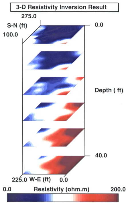
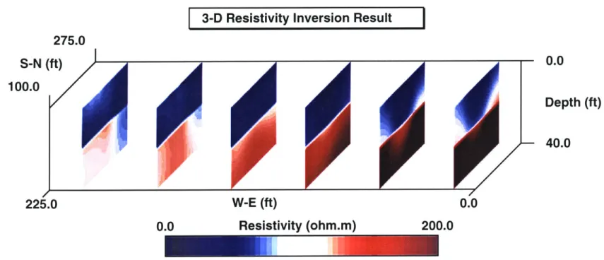
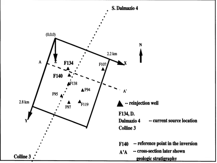
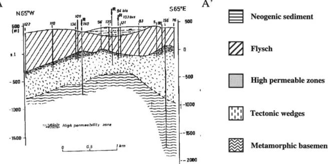
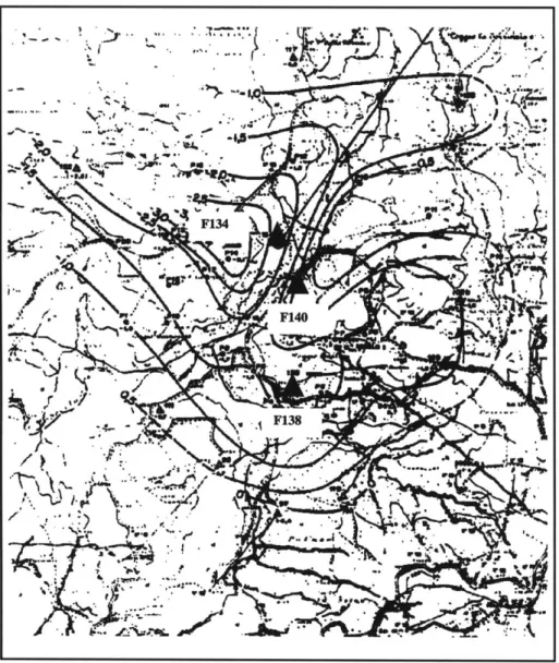
Finally, our inversion techniques are successfully applied to various geoelectric field measurements. The first example applies the 3-D d.c. resistivity tomography to characterize subsurface soil properties in an effort to understand the transport mecha-nisms that have been involved in drinking water contamination in the Aberjona River of Woburn, Massachusetts. The inversion result correlates well with other geophysical results at the site (GPR sections and cone penetrometer logs) and extrapolates the sparse stratigraphic information into a full 3-D model of the study area. The second example uses the 3-D d.c. resistivity tomography to monitor changes in subsurface electrical resistivity caused by the movement of water and the conversion of water to steam in the Larderello-Valle Secolo geothermal field in Italy. Comparisons of the re-sistivity anomalies obtained from two surveys conducted in 1991 and 1993 indicate a correlation between the changes in resistivity and the water re-injection history. The results show that it is possible to evaluate and detect the re-injection of fluid through systematic observation of electrical resistivity at the site. The third example uses the

3-D d.c. resistivity tomography to map underground limestone caves in Barbados,

West Indies. The inversion successfully identifies the known caves and a previously undiscovered cave. In the last example, the 3-D electrical Self-Potential tomography is used to investigate groundwater contamination associated with a jet-fuel leakage at Massachusetts Military Reservation in Cape Cod, Massachusetts. The inversion locates and describes the shape of the contaminant plume which matches well the plume geometry obtained from drill-hole samples.

Thesis supervisor: F. Dale Morgan Title: Professor of Geophysics

Acknowledgment

There are many people whom I wish to thank for their influence on my life and research. My first debt of gratitude is to my thesis advisor, Prof. F. Dale Morgan, who encouraged me to develop a broad range of research interests and stimulated me with endless scientific curiosity. His effort has also brought me unique opportunities to get involved in some worldwide scientific interactions especially those with colleagues in the Caribbean islands with whom I shared not only environmental geophysics knowledge but also the joy of life. Over the course of my thesis research, his advice on every aspect of my research, such as selecting the topic, pursuing the goal, and presenting the work, made the completion of this thesis possible.

I am also indebted to Prof. Nafi Toks6z who supervised my research during the first two years of my study. His ceaseless efforts have provided the students and staff at ERL a unique research and educational environment. His support and encouragement during my first two years of study were invaluable. I owe another debt of gratitude to Dr. Bill Rodi who was always there to offer advice when my work needed help. Almost every aspect of the geophysical inverse theory I have learned in the past years was a great result of working with Bill. His broad range of experience and knowledge in the inverse theory was critical to the progress of my research. His scientific curiosity contributed greatly to the development of this thesis.

I would like to take this opportunity to thank other members of my dissertation

committee, Prof. Harold Hemond and Prof. Robert Van Der Hilst, for their friendly attitudes, encouragement, and helpful feedback. I am also grateful to Prof. Tom Jordan, Prof. Ted Madden, and Prof. John Southard, for the great scientific guidance, conscientious support, and endless patience they provided during my general exam period. Their insight into a wide range of scientific problems opened my eyes. I will benefit from their influence throughout my entire scientific career.

As a full-time student I was sponsored by a numerous funding resources including the Department of Energy, the Environmental Protection Agency, and the Borehole Acoustics and Logging Consortium at ERL.

Thanks also go to Dr. Randy Mackie for his great help and friendship during my first two years of research. His guidance was critical to the progress of my general paper. I am also grateful to Dr. Arthur Cheng who brought me to the ERL and offered much advice on my research.

I am thankful for the friendship of fellow ERLers (past and present); Abdulfattah Al-Dajani, Sara Brydges, Dan Burns, Naida Buckingham, Wei Chen, Ningya Cheng, Chantal Chauvelier, David Cist, Wenjie Dong, Chuck Doll, Bob Greaves, Matthijs

Haartsen, Liz Henderson, Xiaojun Huang, Matthias Imhof, Jonathan Kane, David Lesmes, Yingping Li, Mary Krasovec, Bertram Nolte, Jane Maloof, Joe Matarese, Oleg Mikhailov, John Olson, Chengbin Peng, Rama Rao, Rob Reilinger, Philip Rep-pert, Shirley Rieven, Francesca Scappuzzo, Feng Shen, Roque Szeto, John Sogade, Sue Turbak, Roger Turpening, Yervant Vichabian, Lori Weldon, Zhenya Zhu, Xiang Zhu, Jie Zhang, and Xiaomin Zhao. Specifically, I would like to thank Ms. Kate Jesdale for reviewing my thesis manuscript.

My greatest debt of gratitude is to those who are closest to me. My mother,

father, and sister always have offered me endless care and love. Their tremendous support and sacrifices are the foundations of my life and work. George Theophanis, my father-in-law, is one of the most insightful scientists I have known, he is capable of discussing almost any scientific issue. Susan Theophanis, my mother-in-law, is always passionate and supportive. Nana Olga, and Ari and Maia Theophanis, have been a great source of love for me. Most of all, I wish to acknowledge my husband, Stephen, who has been a great inspiration to me throughout our years together. His tremendous help, scientific insight, and stimulating discussion cannot be measured in the preparation of this document. His brave attitude towards life encourages me to face any challenge.

Contents

1 Introduction

1.1 Background . . . . 1.2 O bjectives . . . . 1.3 Thesis Plan . . . ..

2 Inversion of D.C. Electrical Resistivity Data - Theory

2.1 Introduction ...

2.2 Formulation of the Inverse Problem . . . ..

2.3 Nonlinear Inversion Using Tikhonov Regularization . . 2.3.1 Comparison of Stabilizing Functionals . . . . ..

2.4 Nonlinear Minimization Algorithm . . . .. 2.4.1 Gauss-Newton Method . . . .. 2.4.2 Nonlinear Conjugate Gradient Method . . . . . 2.4.3 Numerical Comparison . . . . 2.5 Conclusions . . . . 20 . . . . 20 .. . . . 25 .. . . . 27 . . . . . . . . 29 . . . . 33 . . . . 34 . . . . 35 . . . . 38 . . . . 39

3 Inversion of d.c. Electrical Resistivity Data - Applications 3.1 Introduction . . . .

3.2 Imaging Aberjona Contamination Site 3.2.1 Introduction . . . .

3.2.2 Inversion Results . . . .

3.2.3 Conclusion . . . .

3.3 Imaging Larderello Geothermal Field . 3.3.1 Introduction . . . .

3.3.2 3.3.3

3.3.4 33 qr

Geoelectrical Survey at Larderello-Valle Secolo . Inversion Procedure . . . . Inversion Results and Interpretation . . . .

onclusins

3.4 Imaging A Limestone Cavern System in Barbados, West 3.4.1 Introduction . . . . 3.4.2 Data Acquisition . . . . 3.4.3 Inversion Results . . . . 3.4.4 Conclusion . . . .

4 Inversion of Electrical Induced Polarization Data

4.1 Introduction . . . . 4.2 Formulation of the Problem . . . . 4.3 Forward Modeling . . . . . 53 . . 54 . . 54 . . 55 . . 57 . . 58 . . . . . . . . 58 . . . . 59 . . . . 60 . . . . 63 . . . . 64 Indies . . . . 65 . . . . 65 . . . . 66 . . . . 66 . . . . 68

Extension of Nonlinear Inverse Theory to the Complex Domain . . Bi-Conjugate Gradient Method . . . . Exam ple . . . .. . .. . . .

C onclusion . . . .

5 Inversion of Electrical Self-Potential Data 5.1 Introduction . . . .

5.2 Formulation of the Forward Modeling . . .

5.3 Inversion Method . . . . . . . . 5.4 Non-uniqueness . . . . 5.5 Field Example . . . . 5.6 Conclusion . . . . 114 . . . . 114 . . . . 116 . . . . 118 . . . . 119 . . . . 121 . . . . 124

6 Uncertainty and Resolution Analysis

6.1 Introduction . . . .

6.2 Uncertainty Analysis via Bayesian Parameter Estimation and Monte Carlo M ethod . . . .

6.3 Uncertainty Analysis via Tikhonov Regularization and Monte Carlo M ethod . . . . 6.4 Augmented Uncertainty Analysis In Tikhonov Regularization . . . . .

6.5 Resolution Analysis Via Model Correlation and The Modulation Trans-fer Function . . . . 6.6 Numerical Results . . . . 6.7 Conclusions . . . . 4.4 4.5 4.6 4.7 98 103 105 106 141 141 146 150 152 155 158 163

7 Optimizing The Electrical Survey 176

7.1 Introduction . . . . 176

7.2 Tomographic Data Acquisition Geometry . . . . 177

7.3 Tomographic Vs. Pseudo-Section Acquisition . . . . 178

7.4 Sensitivity Analysis . . . . 179

7.5 Model Correlation Analysis . . . . 180

7.6 Conclusion . . . . 181

8 Summary and Conclusions 189 8.1 Conclusions and Contributions . . . . 189

Chapter 1

Introduction

1.1

Background

Geophysical surveys are used to remotely sense the physical properties of the earth to provide specific knowledge of the subsurface for a wide range of applications such as oil exploration, mineral prospecting, groundwater mapping, and environmental con-tamination detection to name a few. There are many geophysical surveying methods available to determine different physical properties of the earth which include geoelec-trical, seismic, gravity, magnetic, electromagnetic, and radar methods. Geoelectrical surveys distinguish themselves from these other techniques through the detection of surface electrical fields produced by electric current flow in the ground.

Geoelectrical survey methods include d.c. electrical resistivity, electrical induced polarization (IP), and electrical self-potential (SP) methods. These methods can be classified by the type of electric source involved in the survey. The d.c electrical resistivity and the IP method attempt to map subsurface properties using an artifi-cially applied current source, while the SP method relies on naturally induced current

sources. This thesis will address issues of modeling and inversion techniques, as well

as the optimization of survey geometry as applied to these three methods.

In the problem of d.c. electrical resistivity, one is interested in finding the

subsur-face bulk resistivity distribution from static electrical measurements obtained on the

boundary of the domain, usually the surface of the earth. It is the most commonly

used geoelectrical method due to the enormous variation in electrical resistivity found

in earth material and to its cost effectiveness . This problem has extensive

applica-tions in mineral deposits prospecting, underground facility identification, groundwater

exploration, geothermal studies, and engineering construction projects.

In the problem of Induced Polarization, one is interested in finding the distribution

of the complex character of low-frequency resistivity in the subsurface. The name

in-duced polarization is derived from the analogy to the polarization of electrodes that

occurs when an electric current is passed between an electrode and a surrounding

ionic conducting fluid (Madden and Cantwell, 1967). It has been observed that when

a current is applied to the ground, the ground behaves much like a capacitor, storing

some of the applied current as a charge that is dissipated upon removal of the current.

In this process, both capacitative and electrochemical effects are responsible. In

com-parison with the d.c. resistivity measurements, the IP method measures the transient

(short-term) variations in electrical potential as the current is initially applied to or

removed from the ground. IP is commonly used to detect concentrations of clay and electrically conductive metallic mineral grains, and it has recently been applied to

the detection of underground environmental contaminant plumes.

In the problem of electrical Self-Potential, one is interested in finding the

dis-tribution of subsurface induced current sources, which may be caused by concealed

geological features of economic or other interests, from the measurement of the

are driven by subsurface electrochemical, electrokinetic, and thermoelectric energies. The method thus bears a close relationship to the IP method. Measurements that uti-lize SP have been found in association with studies of groundwater movement related to leakage of dams, dikes, canals, reservoir floors, and other contaminant structures (Corwin, 1990). Other examples of SP investigations include the evaluation of heat flow associated with geothermal activity and certain biologic processes.

While each technique is designed to detect different information about the subsur-face earth material, the physical phenomena of these three geoelectrical techniques are coherent and can be modeled jointly using Ohm's law and the conservation of current. This transfers into a second-order elliptic equation with either a spatially variable coefficient corresponding to the resistivity (bulk resistivity in the d.c. re-sistivity case; complex rere-sistivity in the IP case) or a variable source term (in the

SP case). Under this model, the inverse problem is defined as the determination of

the variable coefficient representing the d.c resistivity, the complex resistivity (IP), or the variable source term representing SP as functions of position given the discrete measurement of electrical potential and certain boundary conditions. This has long been a difficult problem in the geophysics community.

The common difficulties among the three methods resemble many other geophysics inverse problems. The nonuniqueness is by far the most prominent factor to be con-sidered. The solutions of geoelectrical inverse problems are necessarily nonunique. Consider for instance the problem of estimating the the spatially varying resistivity structure as a function of position. Because the resistivity is a continuous function which, in principal, consists of an infinite number of variables, it is impossible to define a unique solution solely from information of a finite number of potential mea-surements on the surface. The nonuniqueness also arises from the lack of knowledge which accounts for the complexity of the real earth: observed potential data always have experimental uncertainty, and the physical theories allowing the solution of the

forward problem are always approximations of a more complex reality.

Geoelectrical inverse problems also exhibit a nonlinear and numerically extensive nature. The electrical potential is nonlinearly dependent on the resistivity structure. Further, the number of parameters in the model must be large enough to allow an accurate simulation of the real earth, and the number of data associated with a moder-ate sized experiment is usually quite large. Thus many theoretical and computational challenges are involved in the successful application of these techniques.

The potential benefit through the application of geoelectrical techniques prompted a long history of extensive modeling and inversion developments for each of these three methods. The following paragraphs will briefly describe the interpretation history of each method, more detailed discussion is reserved for later chapters.

From the pioneering work of the early 1930's through the present day, there has been steady evolution in d.c electrical resistivity inversion technology. In early work between the 1930's and 1950's, efforts were made primarily on the interpretation of resistivity data over a 1-D layered earth using a curve matching technique based on Hankel's Fourier-Bessel formula (Slichter, 1933; Pekeris, 1940; Vozoff, 1958). Issues of the uniqueness and stability were not considered. Later, numerical algorithms using inversion methods on a trial-and-error basis was introduced to 1-D and 2-D resistivity interpretation (Madden, 1967; Coggon, 1971; Mufti, 1976; Dey and Morrision, 1979). Beginning in the late 1970's, more sophisticated numerical modeling for 2-D and 3-D earth models which permitted higher accuracy and resolution were developed. They include the integral equation approach to solve for simple prismatic inhomogeneities (Hohman, 1975; Yang and Ward, 1985; Eloranta, 1986; Beasley and Ward, 1986), the alpha center approach for solving uncomplicated structures (Petrick et al., 1981; Shima, 1990), the finite-element approach (Sasaki, 1992), the finite-difference ap-proach (Dey and Morrison, 1979; Park and Van, 1991; Ellis and Oldenburg, 1994b),

and the network analogy approach (Zhang et al., 1995) for inhomogeneous media. These methods emphasized the ability to calculate the anomalies caused by com-plex 2-D or 3-D structures, they usually required extensive computation and a large number of iterations based on a Newton-type scheme. Even with the approved de-velopment of the mathematical theory in handling complex structure, they are still limited by the computational burden. Some of these methods touched on the use of damping or smoothness to get a stable solution in dealing with the nonuniqueness, but how to properly constrain the model was not fully understood.

The interpretation of IP data was developed in conjunction with the d.c. resistivity interpretation, but with far less success. Until fairly recently IP interpretation was mainly qualitative. Attempts were usually made to plot the change of apparent bulk resistivity with frequency but ignoring the phase shift associated with IP effect (Hallof,

1957; Madden, 1967). Methods for numerically inverting IP data were found to be

sparse in the literature. The most common approach was to invert time domain IP data into an intrinsic chargeability distribution, defined as the ratio of the secondary voltage measured immediately after the current is turned off to the primary voltage measured while the current is on (Pelton et al., 1978; Rijo, 1984, Oldenburg and Li, 1994). There was no successful inversion technique available which could extract more information from the IP data.

Methods for Self-Potential data interpretation were developed independently from the d.c resistivity or IP in past decades. Older methods were mostly based on po-larized simple geometry bodies (de Witt, 1948; Yungul, 1965; Paul, 1965). After Marshall and Madden (1959) and Nourbehecht (1963) who related the solution of electrical potential to the primary coupled flows, research was focused on deriving the potential anomalies produced by the suspected thermoelectric, electrochemical, and electrokinetic sources by taking them as simple dipping dipoles contained in a medium with a simple resistivity structure (Sill, 1983; Fitterman, 1984). All of

these methods were limited to forward modeling, there was no inversion technique

available at the time. This slow progress can be partly attributed to the lack of

practical techniques for the inversion mostly caused by questions of how to constrain

nonuniqueness.

The focus of today's research in geoelectrical imaging has been the development

of efficient inversion algorithms for generating 3-D images of subsurface resistivity

or current source structure. Relatively little work has been done on the problem of

quantifying the accuracy and resolution of such images, i.e. to what degree do the

images represent the actual medium. These accuracy and precision questions must

be answered for geoelectrical imaging to become a practical technology. To further

enhance the geoelectrical imaging method, optimization of the survey geometry is

also a key issue, however, relatively little work has been done on this topic in the

past.

1.2

Objectives

The objectives of this thesis are the following:

e Develop a better inversion method for 3-D d.c. electrical resistivity.

e Extend this inversion method to the 3-D electrical Induced-Polarization and the 3-D electrical Self-Potential inverse problems.

e Characterize uncertainty and resolution associated with the inversion.

9 Develop an optimized electrode array to enhance the resolution and accuracy

* Bridge the gap between geoelectrical inversion theory and the applications by

applying our inversion algorithms to various real geophysics problems.

1.3

Thesis Plan

The topics presented in the objectives will be covered in the individual chapters of

the thesis as follows:

Chapter 2 discusses the generalized inversion methods used to treat the

nonlinear-ity and nonuniqueness of the 3-D electrical inverse problem. I approach the solution to the inverse problems in two parts. First, I present the generalized inverse theory

used as a framework to solve for the unknown electrical parameters. A minimization

condition is defined which combines the misfit between observed and calculated data

with an imposed smoothness constraint on the reconstructed model. This yields a

model with minimum structure: i.e. it is the most featureless structure that fits the

data. I implement this minimum structure approach using the method of Tikhonov

regularization with a differential operator. I examine the possible form of the

dif-ferential operator and will show that, for the electrical resistivity inversion, the best

explicit form of the operator performs a second derivative operator over the region of

the model. I demonstrate the type of regularization which produces minimum

struc-ture models that can vary in the degree of smoothness versus the fit to data. The

second part of the solution is to develop an efficient numerical technique to solve the

inverse problem. I present a nonlinear iterative method using the nonlinear conjugate

gradient method and compare its efficiency with the commonly used Gauss-Newton

method. I show that the efficiency of the method depends on the preconditioning, which controls the search direction of the minimization scheme, and experiment with

Chapter 3 details the implementation of nonlinear electrical tomography for the d.c resistivity problem. From the application point of view, perhaps the most important

objective is to demonstrate that the method can be applied to the real earth. I

therefore apply nonlinear 3-D d.c. resistivity tomography to three field data sets.

The first data set was collected from the Aberjona River in Woburn, Massachusetts.

The goal of the resistivity survey is to characterize the soil structure around the

river in order to understand the transport mechanisms that have been involved in

the contamination of drinking water. Inversion results from the resistivity survey is

correlated with ground penetrating radar data and cone penetrometer information.

The second experiment was performed in the Laderallo Geothermal Field in Italy.

The objective is to relate the variations in resistivity with position and time to the

re-injection history. A particular inversion procedure will be developed to extract the

variation of resistivity as a function of time. The third experiment was performed at

the Harrison's cave in Barbados, West Indies. The objective of the study is to detect

underground limestone caves in an effort to understand the cavern structure in order

to facilitate surface construction activities. I invert data from this experiment and

show that our resistivity tomography technique can be very useful for cave or other

underground facility mapping.

In chapter 4 I extend the theory of 3-D d.c. electrical resistivity tomography

to Induced Polarization inversion. The parameters that are used to describe the

IP effect are complex resistivity values. Under this definition the inversion will be

carried out in the complex domain. From a synthetic example, with the 'true' complex

resistivity value measured from a laboratory experiment, I show that IP tomography

can be utilized to detect contaminant plumes, even with weak concentration, where

d.c resistivity is not effective.

In chapter 5 I extend the inversion theory to the electrical self-potential problem

generated by fluid flow or other origins. I investigate the strong nonuniqueness

prop-erties of the problem, and provide means to reduce the nonuniqueness by various constraints. The method is then applied to map a jet fuel contamination plume at

the Massachusetts Military Reservation in Cape Cod, Massachusetts.

An inversion is incomplete without the analysis of uncertainty and resolution.

This topic is discussed in chapter 6 where I develop a methodology to assess the

uncertainty and resolution analysis of electrical inversion methods.

As a consequence, chapter 7 discusses the optimization of electrical surveys.

Sen-sitivity analysis combined with the uncertainty and resolution analysis provide

guide-lines for the design of geoelectrical field surveys.

I summarize the work and results of the thesis in chapter 8, and discuss future

work directions which could utilize and enhance the capability of our nonlinear 3-D

Chapter 2

Inversion of D.C. Electrical

Resistivity Data

-

Theory

2.1

Introduction

The d.c. electrical resistivity method is a principal geophysical exploration technique which has been used extensively for subsurface characterization. The implementation of the method consists of injecting current into the ground, measuring the electri-cal potential at intervals on the surface or in boreholes, and from those measure-ments deducing the subsurface resistivity distribution. Because the instrumentation is simple and the data acquisition is straightforward, the method is extremely cost effective. Important applications include mineral deposits prospecting (Keller and Frischknecht, 1966; Burger, 1992), groundwater exploration (McNeill, 1990; Medeiros and Lima, 1990), geothermal studies (Burger, 1992) and engineering construction projects (Bogoslovsky et al., 1979; Shima, 1992). Recently, this method increasingly has been applied to environmental protection surveys because of its non-invasive

property. The applications include general hydro-geological mapping (Okko,1993), monitoring contaminated fluid migration (Blum, 1989; Van et al., 1992; Spies and El-lisi, 1995), mapping the extent of landfill areas (Carpenter et al, 1990) and detection of contaminant plumes (Mazac et al., 1990; Buselli et al, 1991)

The electrical resistivity of geological materials depends on mineralogy, clay con-tent, pore fluid, permeability, conducting metal concon-tent, and other properties of the materials. The resistivity value of different geological materials can vary from 104 Q.m(Pyrrhotite) to 10"Q.m (dry limestone), a range in values that may be the widest of any common physical property of earth materials. The electrical resistiv-ity method is ideally suited for the task of detection of chemical contamination. The resistivity of some chemical contaminants may be much in contrast with the surround-ing natural materials, this contrast makes the resistivity method the most sensitive in discerning contaminants from groundwater. Even when the resistivity image does not reveal the presence of chemical contaminants directly, it can provide valuable information on soil properties that control the transport of chemical contaminants.

The task of the d.c. electrical resistivity inversion is to solve for the subsurface resistivity distribution using the measurements of electrical potential on the earth's surface or in boreholes. This is a difficult problem on many levels. One major diffi-culty encountered is that such an inverse problem is ill-posed. The ill-posedness comes from the fact that the number of measurements is always finite while the unknown subsurface electrical property distribution is a continuous function which contains in principle an infinite number of variables. It is impossible to construct a solution that is stable and unique based on fitting data alone. Therefore solutions must incorporate some a a priori information or be regularized in order to be stable and meaningful against the noise in the data. Since such a priori information or regularization is usu-ally difficult to obtain directly from the geological reality, it is subjected to personal bias. Deciding which a priori assumption or regularization criterion is appropriate for

the geoelectrical inversion remains a problem. The other major difficulty associated with the inversion is a result of the problem's nonlinear and numerically intensive nature. Since, in practice, a 3-D model always involves a large number of model parameters and data sets, the forward modeling entails solving many matrix systems. Further, for the d.c. electrical resistivity problem, because the observed electrical potential data are nonlinearly dependent on the subsurface resistivity parameters, iterative methods are needed to obtain the inversion solutions. Owing to this compu-tational difficulty, methods for geoelectrical inversion were mostly restricted to 1-D

(Inman, 1975; Parker, 1984) or 2-D (Pelton et al., 1978; Tripp et al, 1984; Smith and

Vozoff, 1984) earth models in the past decades, only a few 3-D model inversions were

found in recent literature (Park and Van, 1991; Ellis and Oldenburg, 1994; Zhang et

al., 1995).

There has been no great success in overcoming the uniqueness problem associated with practical data. A very common approach is restriction of the solution to the class of models consisting of a small number of parameters. In the past, most methods for d.c. resistivity inversion (e.g. Inman, 1975; Vozoff and Jupp, 1975) used coarsely parameterized models (e.g. large layers or blocks) to make the problem well-posed. These solutions suppress significant structures and can hardly match the geological reality. A more objective approach that allows finely parameterized model was de-veloped by Parker (1984) using bilayer expansion of Green's function on a 1-D earth model. He introduced some smoothness constraints to eliminate the rapid unstable oscillation of the resistivity values that are caused by the non-uniqueness of the prob-lem. Since the bilayer expansion was formulated based on a simple layered model, his approach was limited to 1-D earth models. Park and Van (1991) and Zhang et

al. (1995) developed a 3-D resistivity inversion based on the maximum likelihood

method (Tarantola and Valette, 1982) using statistical information to constrain the models. The method philosophically requires full statistical knowledge of the model parameters. However, in practice, such information is often unattainable. Therefore

the statistical information was often replaced by a uniform damping weighted on each

model parameter which makes the method effectively the same as the conventionally damped least square method.

The approach presented in this paper is based on Tikhonov regularization (Tikhonov,

1977). The method finds solutions by emphasizing the importance of the spatial

cor-relation of the model parameters. It seeks spatially smooth (or "minimum structure") solutions of the inverse problem. The basic motivation for seeking smooth models is

that we do not wish to be misled by features that appear in the model but are not

essential in matching the observations. Other models which satisfy observations but

contain more complicated structures will be far more provocative and attractive than reality. This approach thus provides a low bond of the model complexity. It

guar-antees that the real profile must be as rich in structure as the inversion solution but

never less complex in structure.

The quest for simple solution is well founded in literature. In the early fourteenth

century William of Occam wrote that "it is vain to do with more what can be done

with fewer " (Constable et al, 1987). What has become known as Occam's razor has

also become a fundamental tenet of modern science: hypotheses should be neither

unnecessarily complicated nor unnecessarily numerous. The minimum structure

ap-proach has been taken by many others. For example, it was taken by Rodi (1989)

in 2-D magnetotellurics and seismic data, by Pilkington and Todoeschuk (1992) in cross-hole seismic tomography, by Scales et al (1990) in refraction seismic profile, by

Matarese (1995) in nonlinear traveltime tomography, and by Jiracek et al. (1987), Rodi (1989), deGroot-Hedlin and Constable (1990) in 2D magnetotellurics.

Additionally, we have justification in physics. Due to the diffusive nature of the

electrical energy, the resistivity measurement does not possess high resolution on

representa-tions of the real earth.

When minimum structure models are sought, the inversion requires insertion of some smoothness constraints which are used to minimize the model roughness. One objective in this chapter is to investigate the effect of the smoothness constraints used in the Tikhonov regularization method. We will compare three commonly used smoothness constraints, i.e. the zeroth, the first and the second order spatial deriva-tives of model parameters. We will show that their effect on the stability of the solution relies on the behavior of the sensitivity function, which is a measure of how the electrical potential outputs change due to a small perturbation in the resistivity model parameters.

The difficulty of implementing such minimum structure regularization on a

3-D inversion depends, in part, on the numerical algorithm used for minimization.

For d.c. electrical resistivity, because of the nonlinearity of the forward problem, iterative minimization schemes are needed to obtain solutions. The nonlinearity may also induce multiple local minima in the objective function used to find minimum structure models that fit the data. Therefore it may be necessary to repeat the iterative procedure by varying initial models for the minimization algorithm. Further, due to the non-uniqueness and uncertainty of the problem, it is desirable to find the full set of acceptable solutions or, at least, find as many solutions that fit the data as possible. In doing so, one needs to repeat the iteration algorithm by varying the a priori model or the smoothness constraint. Most current resistivity inversion algorithms are solved by an iterative linearized procedure which corresponds to the Gauss-Newton method (e.g. Park and Van, 1991; Zhang, et al, 1995). It starts from an initial model, then estimates a perturbation of the current model based upon the Taylor expansion. This process is then repeated until the solution converges. This method suffers from slow convergence at the early stage of iterations. It has been shown that it may take tens of hours of CPU time on a high speed workstation to find

a single inversion solution on a small (20x20x10) model (Ellis, 1995). A faster and more robust algorithm is very desirable for extensively studying the uncertainty and the resolution of the problem and to benefit the 3D geoelectrical method in future environmental and engineering application.

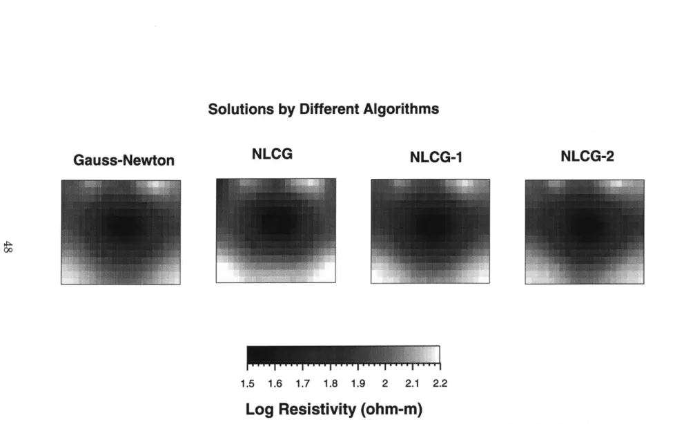
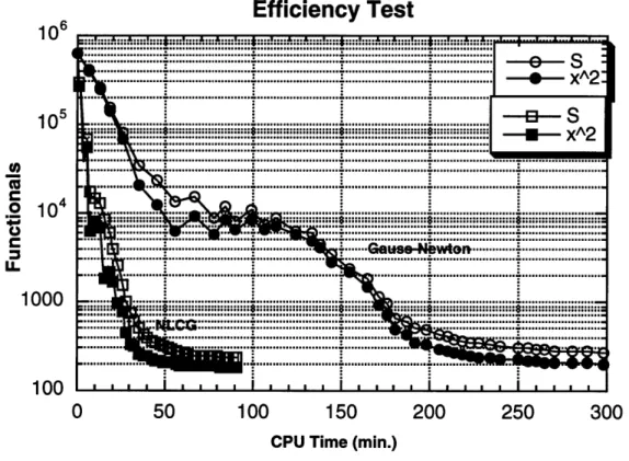
The second objective in this chapter is to investigate a more efficient algorithm based on the conjugate gradient method to solve the nonlinear minimization. We will show that with an appropriate pre-conditioner our algorithm requires fewer computer resources than the Gauss-Newton method, and its superiority will become important when the initial model varies widely from the true model.

2.2

Formulation of the Inverse Problem

A practical d.c. electrical resistivity inverse problem may be defined as: given a set

of electrical potential measurements d = (di, d2, ..., dm) made at the surface or in

boreholes, determine as much information as possible about the subsurface electrical resistivity. This may be written via an equation,

d = G(m) + e (2.1)

where d E EM is a vector representing data in the Euclidean space of dimension M, m = m(x), is the unknown resistivity function, G is a forward modeling operator

which maps the model space to the data space, and e is an error vector. To allow general spatial variations in resistivity and, at the same time, force resistivity to be positive everywhere, we may define m as a function of 3-D position, x, whose values are the logarithm of resistivity, i.e. m(x) = log p(x). In practice, the function m is sampled on a dense grid, m E EN

electrode and the source current density

j(x)

can be written

j(x) = Jo [e+(x) - e-(x)] (2.2) where J0 is the total source current and where e+ and e_ represent the spatial

dis-tribution of the two electrodes. Typically, each electrode is small compared to the spacing between electrodes and e+ and e_ are each taken to be concentrated at a point, e.g.,

e+(x) = 6(x - xo) (2.3)

where (xo) is the electrode position, and 6 is the Dirac distribution.

The forward modeling operator, G, is defined implicitly by the current-conservation equation

V-

(

()VV(x))

=

-I(x)

(2.4)

where I(x) is the current source and V(x) is the electric potential field. Electrical potential V(x, y, z) is subject to appropriate boundary conditions. On the surface of the earth, it is necessary to use the Neumann boundary condition, Bv/ aft = 0,

where n is the direction normal to the boundary. On portions of the boundary inside the earth, an exact boundary condition is not available but various approximate boundary conditions including Dirichlet and mixed boundary conditions (Day and Morrison, 1979; Zhang et al., 1995) can be used. For numerical simplicity, we assume that the model boundaries are far from the source and receiver so that a Dirichlet boundary condition, v = 0, can be used.

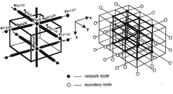
To solve Equation 2.4 numerically, we use the transmission network analog de-veloped by Madden (1972) to discretize the 3-D model into a network that consists of network node, boundary nodes, and impedance branches (Figure 2-1). We define voltage nodes at the top center of each medium block, and the impedance elements,

R2, RY, and R,, at the network branch. RX, Ry, and R2 are functions of the

re-sistivity and the dimension of the network cells. Current sources can be placed at any network nodes and the potential is defined at every node. The governing equa-tion(Equation 2.4) applied to the network results in a linear system of equations:

Ky = s (2.5)

where v is a vector of the potentials at the network nodes, s is the current source vector, and K is a real, symmetric, and positive-definite matrix which depends on the resistivities and dimensions of the network cells. For a potential measurement d at receiver number ir, we can write,

d = G(m) = Cirv (2.6)

where C, = (0, ..., 0, 1, 0, ..., 0), 1 is ir-th the component which corresponds to the

location of the receiver. To efficiently solve the forward problem (Equation 2.5), a linear conjugate gradient algorithm with incomplete Cholesky decomposition is used (Zhang et al., 1995).

Since d is finite-dimensional while (in theory) m is infinite-dimensional, the inverse problem (Equation 2.4) is ill-posed, i.e. unique, stable solutions cannot be obtained solely on the basis of fitting the data. It is necessary to incorporate a priori data or preferences in order to define a unique solution.

2.3

Nonlinear Inversion Using Tikhonov

Regular-ization

There is little success in overcoming the uniqueness problem associated with practical data. The Monte Carlo method, in which a huge number of randomly generated

models are tested against the data, has been used for resistivity (Sternberg, 1979) and magnetotelluric (MT) (Jones and Hutton, 1979b) soundings in an attempt to characterize all models which agree with the observations. Such computations can never be exhaustive.

Another approach to overcome the nonuniqueness is to incorporate some priori information in order to define a unique solution. Classical remedies that advocate

a priori preference into the model fall under two classes. One class assumes that the model parameters are random variables so that statistical information can be introduced to constrain the model. Important approaches include: Bayesian inference (Duijndam, 1988); stochastic inversion (Franklin, 1970), and the maximum likelihood method (Tarantola and Valette, 1982). The second class assumes some "regularity" properties of the solution such as a constraint on the spatial smoothness of the model parameter. This idea is familiar from the modern methods of data interpolation. For example, cubic spline interpolation describes the curve passing through a given series of measurement points with the smallest possible roughness. The original idea of a penalty for complexity seems to be due to Tikhonov, who named the general procedure "regularization", introducing it in order to overcome mathematical difficulties in the theory of ill-posed problems. (Tikhonov and Arsenin, 1977).

Tikhonov regularization defines a solution of the inverse problem that fits the data but also has minimum possible structure. It is our contention that regularization has enormous practical benefits in the interpretation of experimental data. In the case of the highly non-unique problems, this technique is very useful because it provides the simplest, or "minimum structure", solutions (Constable et al, 1987). It is also important to note that the methods in the first class, such as Bayesian inference, stochastic inversion, and the maximum likelihood method, philosophically require full statistical knowledge of the model parameters. However, often in practice, when such information is unavailable, these methods impose some smoothness constrains

which makes them effectively the same as Tikhonov regularization.

Using a least-square criterion, Tikhonov regularization defines a solution that is a joint minimization of data misfit and a "stabilizing functional":

= (d - G(m))TR1(d - G(m)) + T(m - mo)TL TL(m - mo) = min (2.7)

where T is the objective functional to be minimized, Rdd is data covariance matrix, L is a linear operator, r is a positive number known as the regularization parameter, and mo is a a priori model. The first term of T is the chi-squared measure of the data misfit. The second term defines the stabilizing functional which measures the spatial roughness of the model. In the stochastic or the maximum likelihood inversion, mo is taken to be the a priori mean of m and L is chosen such that (LTL)- 1 = Rmm

is an a priori covariance of m. In a minimum structure approach, L is a differential operator and mo is taken to be a simple a priori model. In practice it is desirable to vary mo so that multiple solutions can be obtained.

Conventionally, the most commonly used stabilizing functionals are:

1, L = , (M - mo)TLTL(m - mo) = dxdydzlm - MOl2 (2.8)

2, L = V, (M - mo)TL T L(m - mo) = dxdydzlV(m - mo)|2 _(2.9)

3, L = V2_{, (M - mo)TL T L(m - mo) = dxdydzIV2(m - mo)1}2 _(2.10)

It is not certain whether any of these options guarantees a well-posed minimization in geoelectrical inversion. In the next section we will discuss this issue.

2.3.1

Comparison of Stabilizing Functionals

Among proponents of the minimum-structure approach, there is no consensus on the best smoothing operator L to use (at least for 1-D models) (Bache et al. 1978).

Constable et al. (1987), Smith and Booker (1988) defined L in terms of the first derivative, as in equation (Equation 2.9). Scales et al. (1990) defined L in terms of the second derivative, as in Equation 2.10. Jiracek et al. (1987), Ellis and Oldenburg (1994) defined L as a combination of both the first and the second derivatives. To investigate their influences on the 3D resistivity problem, we compare the three sta-bilizing functionals described in Equation 2.8 - Equation 2.10 both theoretically and numerically.

We know that in equation (Equation 2.7), when T is minimized, its first order partial derivative with respect to m is zero yielding,

A R [T (d - Gr^n) + r-L T L( M^ - mo) = 0 (2.11)

where r^ is the solution at which W(rii) is minimized. A is the sensitivity operator, or Fr6chet derivative which measures how data changes to a change of resistivity model. For a discrete model, A is the matrix

aGi

Aij = (2.12)

8mi

Park et al. (1991) derived that the sensitivity matrix is given by the inner product of the current density (J,) from a point source at the transmitter and the current density

(J,) from a point source at the receiver integrated over the perturbed volume,

Ai ~ f pJs - Jrd3

(2.13)

In the 3-D problem, since the current distribution from a point source approaches infinity at the source, this sensitivity function has singularities at the location of source and receivers. These singularities could result in a large variation in model space given a small perturbation in the data. This aspect of the physics must be accounted for in the regularization method.

solution model fn and the sensitivity matrix A,

LTLi = LTLmo + T-AR-'(d - Gfn) (2.14)

Therefore, when L is an identity, the solution model in^ equals mo plus a linear com-bination of the sensitivity matrix multiplied by the data residual. When L is the first order spatial derivative operator, the Laplacian of fn is a linear combination of the sensitivity matrix multiplied by the data residue. When L is the second order spatial derivative operator, the Laplacian squared of fn are a linear combination of the sensi-tivity matrix multiplied by the data residual. To test which choice of the stabilizing functional yields a stable solution, we design a simple synthetic test problem.

The model is a conductive block (1Q.m) buried in a homogeneous half space (100Q.m) (Figure 2-2). The model is parameterized as Logio resistivity and dis-cretized into 21x21x15 elements with 10 m spacing. The (1Q.m) conductive block is discretized into 7x7x3 elements. 25 receiver electrodes are placed on the surface using the pole-pole configuration, among which nine of them are also used as current electrodes. A total of (9x24=216) observations are produced by forward modeling and 3% random Gaussian noise is added to the data.

To investigate which smoothness operator gives a better minimum structure model, we compare inversion results obtained by different smoothness operators, all fit data equally

(X

2 _{= 216). The results for an inversion obtained using the zeroth, the first} and the second order regularization are shown in (Figure 2-6). The one with the zeroth order regularization has large resistivity variations in the vicinity of source and receivers indicating that the singularities in the sensitivity functions are not suppressed by this stabilizing functional. The first order regularization yields better results; however, the surface artifacts are still seen in the resulting model. The second order regularization successfully suppresses the surface artifacts, giving the smoothest result.

For a given stabilizing functional, the amount of smoothing done is more or less arbitrary and left to subjective judgment. Previous studies (Backus and Gilbert,

1970; Parker, 1984) indicate that when noise contaminates the data there is a

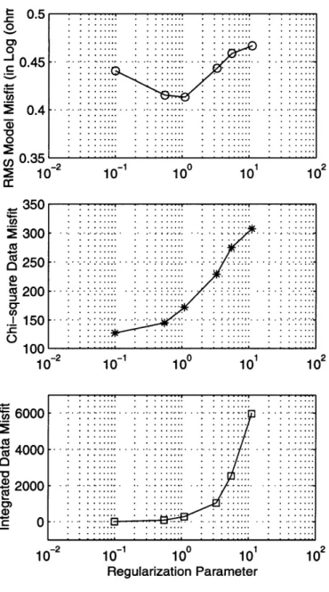
trade-off between the data misfit and the model roughness. By varying the regularization parameter T, _{a trade-off curve (Figure 2-3) is generated using stabilizing functional}

Equation 2.10 as an example. Three points, T1,T2 and 73, are selected from the curve and their associated models are reconstructed and shown in (Figure 2-4). It is found that when the model is too smooth ( when r = 5.5), it can not fit the data very well

(x2 _{= 275). As r is lowered (r = 1.1), the model has a smooth structure and provides}

a better reconstruction (X2 _{= 176). Over-fitting data (x}2 _{= 130 at r = 0.1) results in}

a rough model which contains incorrect surface anomalies.

We now ask ourselves, which -r is the optimum choice? To answer this question, we display the RMS misfit between the solution and the true model and the RMS x2

data misfit as functions of r in Figure 2-5. It is found that there is a minimum model misfit with the corresponding value of r = 1.1 (top). Because this value of r gives

the lowest model misfit, it is considered to be an optimum choice. Unfortunately in practice such comparison of the RMS model misfit is not available because true models are not known. Therefore one must seek other means for choosing the regularization parameter r. If we look at the curve of X2 _{data misfit against the regularization}

parameter T _{(middle) we find there is a slope change in the data misfit curve when} T _{reaches its optimal value. By integrating the}

_x

2 _{data misfit with respect to r the} change in slope is enhanced, as shown in the same figure (bottom). For the segments of the X2 _{data misfit curve that are below this point relatively unconstrained solutions}

are obtained for the inversion indicating a leakage of data noise into the solution. Even though the data misfit is small, the solution is unreliable and the associated model misfit may be large. For the segments of the X2 _{data misfit curve above this}

point, especially for a very large r, inversion solutions are highly constrained and over smoothed, which may result in poor model fitting. This change in slope in the

data misfit curve may serve as a good indicator for picking the optimal regularization parameter, r. In solving a traveltime tomographic problem, Philips and Fehler (1991) have found a similar behavior of the optimal regularization coefficient.

In the case where data contain random Gaussian noise, the expected value of

X2 would be equal to the number of independent data. When x2 _{is greater than}

the number of independent data, the data have not been fully explained by the hypothesized model. This implies that either the inversion scheme is not applicable or the geometry of the model cells is inappropriate. More detail in the data may be fitted if a more complex model is used. In contrary, if x2 _{is smaller than the number}

of independent data, either the estimated variances of the observations have been overestimated (Wiggins, 1972; Inman, 1975) or the inversion is fitting the noise in the data (Inman, 1975).

2.4

Nonlinear Minimization Algorithm

In the preceding sections we have defined the solution of the resistivity inverse prob-lem by minimizing the objective function T in Equation 2.7. Since the forward modeling operator G depends nonlinearly on m, T is non-quadratic and an iterative minimization is required.

In this section we will investigate two algorithms for minimizing the objective func-tional, i.e. the Gauss-Newton method, and a nonlinear conjugate gradients method.

2.4.1

Gauss-Newton Method

The Gauss-Newton method is based on expanding G in a Taylor series and calculating the model correction at each iteration on the assumption of local linearity. By Taylor expansion, we have

G(m + 3m) = G(m) + Aom (2.15)

where we have ignored higher order derivatives. Thus the value of T predicted by Equation 2.7 is

T(m + 6m) = (d - G(m) - Aom)TR-1(d - G(m) - Aom) +

r(m - mO +

om)TL

T L(m - mo + 6m) (2.16)

With this approximation, T depends quadratically on 3m and is minimized by setting

O'J/06m = 0. Thus

om

is found by solving

6m = (A TR-A + rLT-L)(A TR-(d - G(m)) + rL T L(mo - m)) (2.17)

The Gauss-Newton method thus constructs a sequence of the models by

mk+1 = Mik +

omk

(2.18)

where

omk

is given by

6mik = (AkTR.A+ - rL T-L)l(AkTR-1(d - G(mk)) + rLTL(mo - Mik)) (2.19)

and a repetition of this process yields successive estimates m1, M2, ... Mik until the

minimum is found.

Solving this system by computing the inverse of the Hessian, (ATR JA + TLTL), requires a tremendous amount of computing resources. Zhang et al. (1995) suggested that one can solve for 3m _{without direct computation of the Hessian matrix by}