HAL Id: hal-02759747
https://hal.inrae.fr/hal-02759747
Submitted on 4 Jun 2020
HAL is a multi-disciplinary open access
archive for the deposit and dissemination of sci-entific research documents, whether they are pub-lished or not. The documents may come from teaching and research institutions in France or
L’archive ouverte pluridisciplinaire HAL, est destinée au dépôt et à la diffusion de documents scientifiques de niveau recherche, publiés ou non, émanant des établissements d’enseignement et de recherche français ou étrangers, des laboratoires
Walrassian models relevant?
Jean-Marc Boussard, Françoise Gerard, Marie-Gabrielle Piketty
To cite this version:
Jean-Marc Boussard, Françoise Gerard, Marie-Gabrielle Piketty. Evaluating the benefits from lib-eralization: are standard Walrassian models relevant?. 89. Seminar of the European Association of Agricultural Economists, European Association of Agricultural Economists (EAAE). INT.; University of Parma. ITA., Feb 2005, Parme, Italy. 909 p. �hal-02759747�
Evaluating the Benefits from Liberalization:
are Standard Walrassian Models Relevant?
Jean-Marc Boussard
1, Françoise Gérard
1, Marie Gabrielle Piketty
11
INRA-CIRAD , 45 bis Avenue de la Belle Gabrielle, 94736 Nogent sur Marne, France
Contribution appeared in Arfini, F. (Ed.) (2005) “Modelling Agricultural Policies: State
of the Art and New Challenges”, proceedings of the 89
thEAAE Seminar, pp. 274 - 290
February 2-5, 2005 Parma, Italy
Copyright 2005 by Jean-Marc Boussard, Françoise Gérard, Marie Gabrielle Piketty. All
rights reserved. Readers may make verbatim copies of this document for non-commercial
purposes by any means, provided that this copyright notice appears on all such copies.
are Standard Walrassian Models Relevant?
Jean-Marc Boussard, Françoise Gérard, Marie Gabrielle Piketty*
Abstract
While measuring the benefits from liberalisation is obviously important, from a theoretical as well as from a political point of view, one may question the validity of the presently widespread Walrassian approach. The latter does not take account of the fact that supply is just as must (and perhaps more) risk as (average) price responsive. Now, it turns out that if (contrary to the strong versions of the “rational expectation hypothesis”), producers do not take their decisions on the basis of equilibrium prices only, then the market, instead of equilibrium, can generate very harmful seemingly random fluctuations. These considerations are incorporated into a par-tial equilibrium model of the world sugar industry, and a GTAP style general equilibrium model of the world economy. In both cases, liberalisation, preventing price stabilisation poli-cies, results in more instability, and a decrease in welfare. Such an outcome is specific of agri-culture and other low price elasticity commodities.
Introduction
Since at least two centuries1, but with a burst in the early 1980’s, an enormous volume of
lit-erature has been devoted to the measurement of the benefits from liberalisation, especially
agricultural liberalisation2. The recent availability of computable equilibrium models – indeed,
a type of model essentially similar to Walras’, but made “computable” thanks to the availabil-ity of data and computing facilities – has boosted energies in this respect, because, in addition of qualitative conclusions regarding the fact that “liberalisation is globally advantageous”, they provide quantitative estimates of benefit, as well as of how is it shared between stakeholders.
In this context, agriculture is not treated differently of any other activity. The focus on ag-riculture is not derived from the sector’s specificity, but only from the fact that after several
* INRA-CIRAD , 45 bis Avenue de la Belle Gabrielle, 94736 Nogent sur Marne, France.
1 The French “physiocrates” are probably among the first to have raised the problem in its generality: although they are now know by their false theory of value, they were authentically “liberal”, claiming the superiority of “natural” markets over any other sort of economic regulation. See Galiani (1770). Adam Smith acknowledged his debt to them. 2 It is difficult not to mention in this respect the pioneering works by Bale and Lutz (Bale and Lutz, 1979; 1981).
round of trade liberalisation, nothing much but agriculture remains to be liberalized. In this respect, the contemporaneous debate is slightly different from what it was in the past: during the 1770’s, Galiani advocated for trade in industrial matters, and protection in agriculture; be-cause “it was not the same thing”. In the 1840’s, Friedrich List (List, 1841) recommended pro-tecting “nascent industries”, while liberalizing agricultural trade, which allowed lowering wages, thus creating comparative advantage... The only point of agreement with Galiani was again that agriculture was different. Nowadays, the only reference to the agricultural specificity is because agricultural policies are inefficient legacies of the past, providing unjustified rents to rich idle farmers. Most modern authors stress the necessity of getting rid of the “agricultural excep-tion”.
Nevertheless, the question arises of the validity of this modern approach. In effect, three main criticisms has been addressed to CGE's models in this respect:
i - The most ‘liberal’ situations depicted through these models are undoubtedly efficient
and Pareto optimal. But they rely on a particular income distribution, resulting from factor scarcity rents, which are not necessarily socially optimal: other Pareto efficient situations,
with a different income distribution, could be deemed socially more desirable3.
ii - Only those commodities which are subject to market exchanges are taken in account in
this approach. Those which for some reason (externalities etc...) are ignored by the market are also ignored in the benefit / cost balances derived from CGE’s. and:
iii - A CGE model assumes markets are functioning properly, i.e. marginal equate marginal
receipt everywhere, producers and consumer adjust theirs plans immediately in response to observable equilibrium prices (hence the reference to “equilibrium”).
Objections i and ii are serious, yet, they can be overcome if models are intelligently made use of: it is an old tradition in theoretical benefit cost analysis to take account of these kind of considerations, even if the corresponding rules for computing “shadow prices” are actually rarely put into practice. Indeed, in such a context, it is relatively easy to modify the original
Walrassian model, or to change governments utility functions4.
Objection iii, by contrast, is much more difficult to overcome. The problem arises because if markets are not equating marginal costs with prices or marginal utilities, then all the solutions extracted from the model are just as meaningless as a bad fiction. There is no point using the model in any way, because it has no connexions with reality...
But how can we assert that these models have no connexions with reality, while most modern economists, although acknowledging the CGE's limitations, nevertheless congregate in
3 An additional difficulty, in this respect, is that solutions in general imply the existence of looser as well as of winner. In welfare theory, it is well known that such situations can be dealt with through compensation: since the gains from winner are greater than the losses from looser, it should be possible for the winner to compensate loser, and keep a benefit nevertheless. Yet, in international relations, it is not very common to have the loser effectively compensated. 4 For instance, a constraint imposing green house gas emissions not to exceed a specified quantity can be introduced... Similarly, a large body of literature has been for long concerned with linear and non linear taxation rules (see for in-stance Atkinson and Stiglitz, 1980).
using them at least as benchmarks, and probably as depicting “long run situations”, after all adjustments have been made? We shall try here to answer this question. First, the theoretical foundations of our argument will be presented. Then, illustrative results from an application will be presented.
I - Theoretical considerations
Apart from monopolistic competition considerations, the main immediate reason for a dis-crepancy between marginal costs and prices is to be found in risk considerations. But risk con-siderations alone would not be sufficient to question the validity of the Walrassian model. Many famous works show very clearly and convincingly that any exogenous risk can be
ac-commodated into a Walrassian framework5. The central argument here is that the market by
itself can endogenously create risk, and maintain it, through dynamic mechanisms. In addition, such a mechanism is not general, but to large extent, specific to agricultural commodities. Let us begin by a discussion of risk effects.
The negative welfare effects of risk
In presence of risk, as it is well known, producers do not equate marginal costs with prices, but
with the certainty equivalent of prices. With prudent producers6, the certainty equivalent of an
uncertain price is normally less than the mean value. The production is therefore lower, and the average equilibrium price higher than it would be expected with marginal costs equating
average prices7. The welfare consequences of such a situation have been the subject of many
discussions. It is not clear who benefits and who suffers, the producer or the consumer. Yet, there is a general consensus that the overall effect is negative, the magnitude of losses encom-passing the size of benefits.
A very natural method to avoid risk is insurance. But for (small) transaction costs, an
in-surance contract is free, replacing an uncertain prospect by its mean8. This would be a very
good reason of neglecting the price risk problem, if insurance contracts were to exist for prices. Yet, such contracts are never offered, despite their obvious social and private utility. This is
5 Especially as soon as contingency markets do exist, but even in the absence of them (in which case, losses of effi-ciency can occur, which would have been absorbed by an insurance market).
6 It is better here to speak of “prudence” rather than of “risk aversion”. There are indications that many farmers (not to speak of other producers) are at least risk neutral (Binswanger, 1980). However, a risk lover may be prudent (see Kimball, 1990), leading to the same ultimate result regarding the sense of the risk premium. Notice also that if produc-ers are risk lover, and bankproduc-ers are risk avproduc-erse, the consequences are also the same.
7 See in particular, among others, Just and Zimmermann (1986)
8 Indeed, it is never completely free, since the service of the insurance company must be rewarded. But this cost can very well be neglected here.
because price risks are special, not satisfying the “law of large numbers” requirements, there-fore “not insurable”. Such an observation leads to the questions of why are price risk specific?
Why are price risks specific?
An obvious reason for the absence of price insurance contracts is the size of the risk for the insurer: if all clients are selling on the same market, in case of less than average observed price, they will claim indemnities all together. There will not exist any contemporaneous compensa-tion between damages and premiums. Now, it is at least theoretically possible for an insurer to diversify this sort of risk both over space, by selling contracts in non integrated markets, and time, because not every year can be bad.
Most of the safety mechanisms which have been recently contemplated to avoid the nega-tive consequences of price risks rely upon this reasoning: for instance, Bale and Lutz (1979) advocate extending international markets on the ground of insurance, because large markets will be less volatile than the presently9 narrow existing ones10. Similarly, the Canadian crop
in-surance scheme is based on the compensation between “good” and “bad” years. But are price risks small and independent through space and time? To answer this question, a prerequisite is to investigate the source of agricultural price volatility.
Where does price risks come from?
The most natural idea in this respect is that risk comes from exogenous shocks, due to climatic or analogous contingencies. This idea is at the origin of all insurance based mechanisms de-signed to alleviate the consequences of risk in agriculture, as those alluded to above. Indeed, nobody can deny the importance of climate and pests in generating individual farmer risk ex-position. It is quite natural to extend the notion to collective markets, hence to prices. In addi-tion, such risks, even “large” at regional level, are obviously “small” and probably “independ-ent” at world level11. These are the conditions for the feasibility of an insurance scheme, as
pointed out by Bale and Lutz. The later would be specially efficient, since it would work auto-matically, without transaction cost, simply by the fact that international prices would be stable. Yet, one can observe that many unsupported and unregulated international commodity prices are very volatile. At the same time, when a careful study is conducted over the source of price volatility for a given commodity, as for instance the famous Roll (1984) investigation of
9 That is, in 1979.
10 Indeed, the heart of their paper is nothing else than a demonstration of the central limit theorem.
11 Here, the quotes for “small” and “independent” refer to the various specifications of the central limit theorem, which differ by the precise meaning given to these words.
the Florida orange juice, it is found that, undoubtedly, climate plays a role, but at the same time, explains only a small share of the volatility12.
What can explain the remaining share of the volatility? An alternative explanation may be found in the mathematical theory of chaotic motion. It is much less optimistic than the previ-ous one regarding the possibility of insurance schemes to cope with price variability. At the same time, it fits relatively well with elementary basic supply and demand theory. Below, we shall see that it also provides a fairly promising explanation of actual observed price volatility. Let us have a look at the basic supply and demand model.
A simple supply and demand chaotic model
Consider a set of linear supply and demand curves. With α and β being the demand curve
slope and intercept, a and b the supply curve slope and intercept, qt the quantity produced or
demanded, pt the equilibrium and pˆt the expected price at time t, if pˆt = pt-1., . then:
a b a p a pt=# t!1+ "! (1)
This is the old Ezekiel (1938) “cobweb” model. If !1
a
" , then there is no limit for pt and qt,
which growth to infinity (by alternate values, since α is normally negative) as time passes. The
explanatory value of this model is low, because one cannot imagine prices and quantities
grow-ing to infinity. There is a special periodic solution for α/a = 1, but nobody can admit such a
situation is general. Now, just consider introducing risk and risk expectation in this model. Let us suppose that producers maximize the certainty equivalent (in Von Neuman’s sense) of profit, given expected price pˆt , and expected price variance !ˆt2. Take for instance pˆt=p~,
constant, while 2
1 1
2 (ˆ )
ˆt=pt!!pt!
" (“naïve” expectations regarding volatility). Then, equation (1)
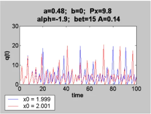
becomes (1bis): ! ! " " + # # + # = # 2 1 ) ~ ( ~ t t q p A a b p p (1bis) with A being the average absolute risk aversion coefficient. Such a formula can easily been im-plemented on an Excel or similar spreadsheet. Figure 1, below, provides an example of the time series it permits to obtain.
Here, we see that highly fluctuating and apparently random series13 are generated by a
completely deterministic process, without any random component. This is the heart of chaotic
12 Hence the idea of predicting the Florida climate from the future price of orange juice, which according to some (Savage 2004), works better than the US meteorological service... Yet, in the case of Florida juice, because of the or-chard geographical concentration over a small region, together with a large share of market, the conditions were ideal for a massive influence of climate over prices.
theory. In addition, the above model is hardly more complicated than an elementary class room scheme, and based on almost trivial behaviour theories: there are therefore no reasons to think it can be less predictive than this elementary theories are... Finally, this model rules out any stabilisation scheme based on insurance. Any tentative to stabilise prices by merging mar-kets in such a context leads to unpredictable results: sometime, volatility is decreased, and even disappears, but in other cases, for “almost the same” parameters, it is increased. It is generally impossible to delineate any region of the parameter space guarantying any specific behaviour of the model.
Yet, an important point must be made in this respect: although the “chaotic” regions of the parameters space are “fractal”, that is complicated, and not necessarily compact sets, there is nevertheless something firm and invariant in the generation of chaotic motion. The latter occurs when one or more equilibrium points do exist, and are unstable (or “repelling”, in the standard dynamic theory language). In addition, there must exist one or more forces (“return spring”) capable of bringing back the system into the vicinity of an equilibrium point whenever it tends to go too far away.
In the above model, the instability of the equilibrium point is warranted by the low de-mand elasticity: here is the main (and genial) Ezekiel (1938) contribution, nowadays quite un-justly forgotten. The “return spring” necessary to bring the system back to equilibrium is risk aversion. This is again an old idea: Knut Wicksell (1898) already made the risk the deus ex ma-china of his business cycle theory. In the present case, the association of Ezekiel and Wicksell results in a theory of commodity price volatility which is mainly specific to agriculture, since
food commodities are certainly the most inelastic demand in the world14.
Figure 1. Constant mean expectation risky cobweb. There is nothing random in this graph… The red
and blue curves are with the same parameters, and start at about the same point. They part one from each other, just as two exponential do.
13 Indeed, although it is chaotic by construction, there does not exist any serious statistical test allowing for a clear dis-crimination between these and “true” random series, for instance Wiener’s random walk processes.
Consequences for measuring agricultural trade liberalisation benefits
If any mechanisms as those described above is at work in agricultural commodity markets, the consequences of liberalisation might be quite different from those expected.
Standard CGE’s and Walratian models do not account for risk. If liberalisation is likely to make price volatility lower, then the corresponding benefits will be underestimated, since lower risk premiums in already “liberal” countries will produce efficiency gains in addition of those resulting from the exploitation of comparative advantages. But if world price volatility is in-creased, or even left unchanged, the risk premiums are likely to increase in presently “pro-tected” countries, even if they remain unchanged elsewhere. Since “pro“pro-tected” countries ac-count for the bulk of world agricultural production, such an increase of risk premiums will by no means be neutral. It remains to be determined to whom the (negative) benefits will accrue. Hence the necessity of “disequilibrium models”, tailored on the same general pattern as of par-tial or general equilibrium models, but modified in order to take account of the above consid-erations, in just the same way as the standard class room equilibrium supply and demand has been converted into a disequilibrium model. In short, the idea is to replace the Walrassian CGE’s models by something a little more sophisticated, grounded on a little more recent Wicksellian theory. Such models could be called “disequilibrium”. The idea can be applied to either “general” or “partial” disequilibrium models, as we shall see now.
II - Illustrations and application
The above ideas have been applied in two recent studies. The first is based on a sectoral model of the sugar market liberalisation, the second, on a world “GTAP” model of the world econ-omy. We shall give here a taste of the results of each of them, referring to the associated publi-cations for further details.
1/ A sectoral model of the sugar industry
The sugar industry carries over a very bad repute among economists: most of the production is independent from market, with preferential prices, and rent generating quotas. Geographically, a large proportion of sugar production is made from beets in temperate countries, while most agronomists congregate in considering tropical regions sugar cane as a better transformer of solar energy. Sugar prices are highly volatile, but, according to the standard mode of reasoning described above, this is a quite natural consequence of a narrow residual market. According to common wisdom, letting the market operate naturally should reduce volatility by a large amount, because governments will cease to sell off useless surplus. There are therefore all the reasons to think that liberalising the sugar market will create very large surplus.
To check this hypothesis, a model of the world sugar industry has been designed by Bous-sard and Piketty (2002). The model is made of a large quantity of submodels, each of which being relatively simple and “classical” in its spirit, the main unknown being the behavior of the whole, when constrained by the necessity of clearing markets.
As for instance in the well known ABARE model of the world sugar industry (Hafi et al. 1998), sub-models are set up for:
i – farmers, when deciding each year how much future contract they will pass with sugar
processing factories15.
ii – Sugar processing factories, when they decide how much future contract to buy from
farmers, and sugar refineries when they decide how much raw sugar will be processed into white sugar.
iii – Sugar processing factories, when, acting as stockpilers, they decide how much sugar to
sell out of their stocks on the spot market.
iv – Refineries and sugar processing factories, when they decide to invest in new capacities
from savings depending upon their past benefits.
For each of these operators, the first order conditions for utility maximization are written, and the model is closed by the necessity of clearing markets at all levels.
Each of these submodels are rather standard, except perhaps in computing processing plants costs, because, in addition of traditional features, a geographical non linear consideration is added up: since the average distance of the center of a circle to the points of the correspond-ing disk is proportional to the radius, the cost of transportation between farms and the proc-essing plant increases as the power 3/2 of processed quantity. A stabilizing effect was expected from this trick. In practice, under reasonable assumptions regarding transportation costs, it never played a large role in results.
15 In effect, farmers pass a sort of future contracts with processing plants, the latter offering to buy the whole produc-tion at current price at harvest time. Farmers decision is then which sugar density of producproduc-tion (i.c., tons of sugar per ha of total agricultural area) do they have to promise. Processing plant’s decision is which agricultural area to prospect.
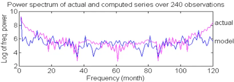
Figure 2. Comparison between predicted (reference run) and actual time series Fourier power spectrums.
For any particular point of these curves, a “high” ordinate value means that the underlying period (as de-fined by the number of month along the x axes16) is “important” in explaining the general shape of the
series. The “actual” series is obtained from 240 first monthly average of the daily series published by Chadwick Investment group, starting May 5th, 1970, ending September 14th 1999.
By contrast, the original feature of the model which played a very decisive role was the intro-duction of risk into the utility functions of each of decision makers: instead of expected profit or utilities, for each representative decision maker, a classical Von Neuman utility function is maximized. In each case, the absolute risk aversion coefficient is computed as the inverse of the average wealth of the corresponding decision maker, thus implicitly assuming on approxi-mately constant relative risk aversion coefficient. In this way, a major characteristic of the het-erogeneity of decision makers is taken into account, since the hethet-erogeneity in wealth can be considered as a summary of all kinds of heterogeneity.
For the results presented here, price expectations are constant (again, as in the class room model above), on the ground that, presently, the volatility of sugar price is so large that nobody can trust the current price, and consider it carries any useful information. By contrast, the ex-pected price volatility is defined as above, as a variance, and measured by the squared differ-ence between two successive prices.
Finally, producers know their current costs, and consider them as the “normal” price. The basic time step is one month. The model has been validated, by comparing the Fourier spec-trum of actual versus simulated white sugar price series (Figure 2: the fit might be deemed poor. Notice however that most sugar models recommending liberalization were never tested at all, and generate completely flat time series still much worse than the present one).
Results show that liberalization, in this context, reduces production and raises average prices. This is not new, and consistent with findings by other models. However, contrary to expectations, it increases rather than decreases the volatility. And since decision makers require large risk premiums, average prices increase much more than with standard models. At the
16 To be precise, the peak at abcissa “20” means a perturbation which occurs every 120/20 month, that is, every 6 month.
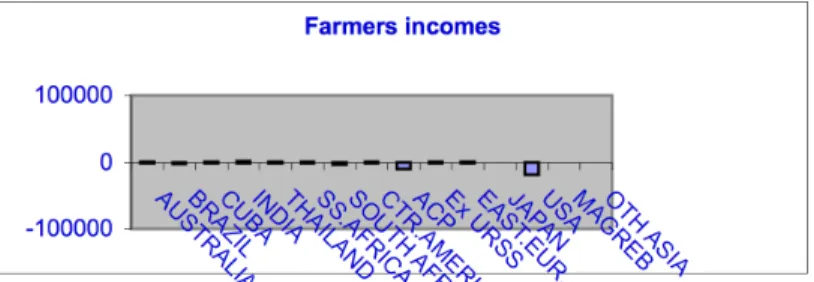
end, most benefits (as measured by profit and consumer surplus) are negative (Figures 3-5; values in 1000 $):
Figure 3. Effects of liberalization on average farmers incomes.
Figure 4. Effects of liberalization on consumers surplus.
Figure 5. Effects of liberalization on white sugar manufacturer incomes.
Such results are quite different from those reported by other authors (for instance Hafi et al. 1998, or Wohlgenant, 1999), using basically the same model, but ignoring risk and volatility... Indeed, here, most of losses come from consumer surplus, which overrun producer benefits. This is consistent with the above reasoning regarding the detrimental effects of volatility. In-deed, the underlying reason behind this conclusion is that the inefficiencies introduced by agri-cultural policies are more than compensated by the benefits from stable prices. “Free trade”,
despite a better use of comparative advantages, is ultimately harmful by precluding the possi-bility of stabilizing domestic policies.
2/ A global CGE model using GTAP data
Thus, introducing risk and unfulfilled expectations in a sectoral model is bound to change con-clusions regarding the desirability of liberalization policies. This is not so surprising, since we are here in the simple logic of the traditional cobweb. The conclusions derived from the class room exercise are straightforwardly extended to this context. At the same time, sectoral models have their own flaws. In particular, they neglect the feed back effects of incomes over demand. Would the above conclusions resist the possibility that increased risk premiums come back as increased incomes and demand? This leads us to consider true CGE’s models.
The same kind of experiment as described above has therefore been conducted (Boussard et al, 2004) with a full CGE model, derived from GTAP. Indeed, care have been taken to, as far as possible, keep all standard GTAP specifications and data. It is thus not necessary to de-scribe the model in detail. Only the changes linked with expectations, risk and accumulation are to be explained. Specifically:
• • The model is recursive – that is, solution for year t is derived from solution for t-1
without intertemporal optimisation (this a very common assumption in GTAP mod-els).
• • Capital is sector specific: it is not possible to shift a combine harvestor into a
nu-clear power plant. Again, this is a very classical assumption. However, in most similar GTAP models, the new capital is allocated to sectors according to some elasticity of new capital supply with respect to profitability (in order avoiding that all new capital be allocated to the “most profitable industry”). Here, the capital supply elasticity is implicitly determined by a risk sensitive process – actually, a simple Markowitz's mean variance portfolio model: one maximizes a weighed sum of expected mean and vari-ance of profitability under constraint of total available savings (Markowitz, 1970).
• • Production of year t is determined by expected rather than by equilibrium prices,
thus creating a cobweb effect into the model. Expected prices and price volatility measures are computed each year using expectation schemes – actually, classical Ner-lovian formulas of adaptative expectations.
• • Because we intended assessing the distributional consequences of risk – assuming
risk premium were distributed as a capital income –, the only major difference be-tween the standard Hertel model and the present one in terms of data is that the household institution has been split into two, “rich”, and “poor”.
Except for these features, the model is completely analogous to other GTAP model, with Armington functions for trade, CES production functions for factors and linear intermediate inputs etc... Most elasticity’s are just copied from Hertel et al. (1995). Indeed, it is so much similar to the original Hertel model that it can be run as a classical standard CGE (although the capital allocation module is still a Markowitz portfolio model, thus introducing an element of risk into even what is called below the “standard model”). Thus, it is possible to assess the consequences of introducing risk and risk premiums into the production/consumption module by comparing results from the “standard model” with those of the “risk model”.
Figure 6. Standard model liberalization effects on rich and poor. Difference between “liberalization” and
“reference”, in % of reference.
Figure 7. Recursive model liberalization effects on rich and poor. Difference between “ liberalization”
and “reference” , in % of reference.
0 10 20 30 40 50 60 70 -1 0 1 2 3 4 5 6x 10 -3 time ( C u r r e n t -r e f e r e n c e ) / r e f e r e n c e %
Poor households utility index Whole World LIBNOLAG 0 10 20 30 40 50 60 70 -1 0 1 2 3 4 5 6 7 8x 10 -3 time ( C u r r e n t -r e f e r e n c e ) / r e f e r e n c e %
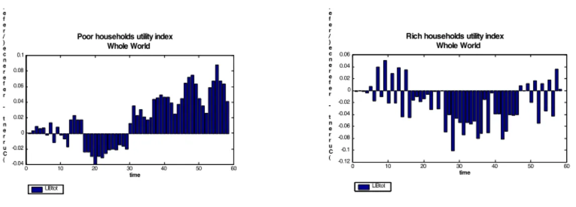
Rich households utility index Whole World LIBNOLAG 0 10 20 30 40 50 60 -0.04 -0.02 0 0.02 0.04 0.06 0.08 0.1 time ( C u r r e n t -r e f e r e n c e ) / r e f e r e n c e %
Poor households utility index Whole World LIBtot 0 10 20 30 40 50 60 -0.12 -0.1 -0.08 -0.06 -0.04 -0.02 0 0.02 0.04 0.06 time ( C u r r e n t -r e f e r e n c e ) / r e f e r e n c e %
Rich households utility index Whole World
This is what was done over a simulation lasting 60 years17. Results are presented on figure 6 for
the “standard” model: this the kind of results generally presented in such exercises18.
Obvi-ously, liberalisation is highly beneficial. Results from the “risk model” on figure 7 are quite dif-ferent: here, the rich are losing while the poor gain, but only after a long time (during which they may very well die!). Notice that the magnitude or gains and losses are not the same in both figures: actually, losses and gains are 10 time greater in the “with risk” than with the stan-dard version of the model. This is again a consequence of the increased price volatility, as visi-ble on figure 8.
Figure 8. Prices of sugar and manufactures with four scenarios. LIBNOLAG and LIBtot refer to
liber-alisation with and without risk and imperfect expectations considerations. REFnolag and REF60 are the corresponding reference runs.
Figure 8 (relative to “sugar” and “manufactures” in the “rest of the world’, but similar graphs could have been drawn for almost all countries and commodities)shows that prices are much more volatile in the “risk” model results than with the corresponding standard simulations. Again scales are not the same in both graphs: on the right panel, price indexes vary from 0. to 3 – which is rather realistic for the free sugar market –, while they vary from 0.8 to 1.3 only in the case of “manufactures”. It reflects the much larger price demand elasticity in the case of manufactures as compared with sugar. Yet, sugar (and other agricultural commodities) volatil-ity is somehow contagious, since, otherwise, given a large demand elasticvolatil-ity, manufacture prices should converge toward equilibrium in the “risk” model, just as they do in the standard case.
It remains to be seen if such a volatility, creating a large number of bankruptcies and starv-ing peoples, is sustainable: most of the time, governments intervene when markets are too
17 In order to be able to make a statistical analysis of results. Notice population is constant in each countries. There-fore, labour is fixed, thus precluding any “forecast” being derived from the exercise.
18 UNCTAD (2004) provides a list of such models, all of them with completely similar results, which is not really upris-ing, since they are all the same, using the same GTAP data and assumptions. Notice however the lost of benefits in year 30, due to the lack of investment, itself a con sequence of the Markowitz savings allocation model.
viously failing. Indeed, such interventions are at the root of the agricultural policies which were put in operation almost everywhere in the world in the aftermath of the “great depression”. One may hypothesize that, since the same cause in the same conditions are likely to lead to the same effects, the occurrence of a series of crisis such as those described by the above “risk”
model would lead to new wave of protectionist policies decided on the ground of emergency19.
Indeed, here is a logical difficulty to test this kind of models and scenarios: it impossible in the modern world to find any example of the absence of government intervention in agricul-ture lasting 60 years. The governments who intended such actions never lasted for so long...
Conclusion
The conclusions to be derived from this set of experiments are numerous. They concern both research strategies and policies.
a) For research strategies:
An obvious consequence of the above presentation is the importance of risk. This is not new. Just (2003) in a very brilliant review paper, reaches the same conclusion: “production econom-ics generally has undergone a major redirection of methodology, replacing primal methodology by dual methodology in the 1970’s. It may be undergoing another transformation toward non parametric approaches presently. Both of these movements have developed a preoccupation with methodologies that assumes risk aversion is non existent. In general practice, the condi-tions of profit maximisation are no longer tested, but simply assumed”. And he points out the numerous false conclusions which are derived from this neglect, especially when long run con-siderations are at stake.
Indeed, if risk is just as important as mean price levels in shaping production and supply, then it is extremely surprising that only a small share of efforts devoted by our colleagues to elicit mean price response be devoted to risk aspects of agricultural production. The present exercise makes a very rough application of standard theory of decision making in presence of risk. It is therefore the more interesting to see how it is important for results: if a minimal ac-count of risk influence yields such changes of perspective, then what would be the conse-quences of a more sophisticated approach?
But the present set of researches goes beyond what was expected by Richard Just: not only the behaviour of individual farmer facing risk is important, but the way risk and expectations are generated. Very few agricultural economists are aware that risk might be generated by other mechanisms than climates and pests, or, with more pretence, “the hand of God”. Yet, climatic and similar risks are minor. Real dangers come from market failures, and endogenous risk. Ac-tually, price risk generated by the market itself, out of any “random” events, is much more
19 Here is another reason, after the neglect of population migration, for not considering the above series as “forecasts”. Our purpose is just to provide a counterfactual experiment.
portant than the ordinary technical risk, which farmers are accustomed to deal with. This is something much more preoccupying, which should attract much more research endeavours than presently done, because it question the whole system of market economy as applied in agriculture.
This last result was central in the mind of the designers of the first US farm bill (Lindsey, 1934): they were accused of “socialism”. Their answer was that they had nothing to do with socialism, but that there were agricultural specific market failures, which required agricultural specific solution – in short, the “agricultural exception”. In their view, this situation was justi-fying the very existence of agricultural (as opposed to industrial) economics. Later on, the demonstration by Nobel prize Theodore Schultz that even traditional farmers were rational gave additional weight to this assertion: if farmers are just as rational as any other entrepreneur, then what is specific in agricultural economics? The above reasoning provides at least one an-swer among others. It is very strange that the profession, at present, does not seems to be in-terested any more...
b) For policy making:
The benefits from liberalisation are even smaller than customarily estimated. Worse, they might be negative. The reason for such a surprising statement is not a radical attitude, as for those who, for ideological reasons, deny the possibility of exploiting comparative advantages. On the contrary, the models presented here are designed upon a very standard neoclassical pat-tern, which leaves plenty of room for the comparative advantages to manifest themselves if they are present. Actually, they are present, as the results of the “standard model” above tes-tify. But the benefits from exploiting comparative advantages have a cost: the increased volatil-ity of prices. In the case of low demand elasticvolatil-ity commodities, the latter leads to losses of effi-ciency, with detrimental effects larger than the benefit derived from comparative advantages.
Would it be possible to overcome these difficulties through insurance schemes or similar devices? The experiences reported above do not permit to conclude, because such schemes are not considered into the models. Yet, the “class room model” presented at the beginning of this paper can cast some light on the question.
First, insurance is not possible. This is not only because, as claimed by insurance compa-nies, a price risk accident affects simultaneously a large number of subscribers. Although the argument is serious for a small insurance company, intertemporal compensation, linked with financial reserves, should make it feasible by a very large company, or a government. The rea-son behind the infeasibility of insurance here is moral hazard. Not the moral hazard tied with information asymmetry between subscribers an insurers, as one might think from a too narrow idea of the possible sources of moral hazard, but the fact that as soon an insurance scheme is offered, the supply parameters are changed, thus jeopardizing all ex ante risk evaluation from the part of the insurer.
If insurance is not feasible, then, why not futures markets, options, and other financial de-vices? Boussard (1996) reports an experience in this respect which tends to show that in prac-tice, this remains to slightly change the parameters of the system (essentially, by changing the average market risk aversion), without modifying its fundamental properties, thus not solving
the problem. By contrast, production and trade quotas could be much more efficient. But these results are still very preliminary, and will, hopefully, be the subject of another papers.
In any case, letting the market manage production is certainly not a sound solution inas-much as agriculture is at stake, and, particularly, when agriculture is very important for the economy, as in developing countries (Timmer, 2000).
References
Atkinson A.B. and Stiglitz J.E. (1980): Lectures on Public Economics, McGraw-Hill.
Bale M. and Lutz E. (1981): Price distorsion in agriculture and their effects. An international compari-son, AJAE 63 (1): 8-22.
Bale M. and Lutz E. (1979): The effect of Trade intervention on international price instability, AJAE 61 (3): 512-516.
Binswanger H. (1980): Attitudes toward risk: experimental measure in rural India, AJAE 62: 395-407.
Boussard J.M. (1996): “When risk generates chaos”, Journal of Economic Behaviour and Organi-zation, 29 (96/05): 433-446.
Boussard J.M. and Piketty M.G. (2002): “Conséquences possibles de la libéralisation des marchés du sucre: deux modèles et leurs réponses, Economie Rurale, 270, 2002/08: 3-18. Boussard J.M., Christensen A.K., Gerard F., Piketty M.G. and Voituriez T. (2004): “May
the pro poor impact of trade liberalisation vanish because if imperfect information?”, Agricultural Economics 31 (2).
Di Costanzo S. (2001): Le rôle du stockage dans la dynamique des prix des matières premières, Thèse, Université de Paris I.
Ezekiel M. (1938): “The Cobweb Theorem”, Quarterly Journal of Economics, 53: 225-280. Galiani F. (1770): Dialogue sur le commerce des bleds, Réédition, Fayard, Paris 1984.
Hafi A., Connell P. and Sturgiss R. (1998): “Market potential for refined sugar exports from Australia”, ABARE research reports, 93-17, Canberra.
Hertel T. et al. (1997): Global trade analysis, Cambridge, Cambridge University Press.
Just R.E. (2003): “Risk research in agricultural economics: opportunities and challenges for the next twenty five years”, Agricultural system, 75: 123-159.
Just R.E. and Zilberman D. (1986): “Does the law of supply hold under uncertainty?”, The Economic Journal, 96: 514-524.
Kimball M.S. (1990): “Precautionary saving in the small and in the large”, Econometrica, 58 (1), January: 53-74.
List F. (1841): Das nationale System der politischen Ökonomie French translation. Système National d’économie politique, Gallimard, Paris, 1998, avec préface et commentaires d’Emmanuel Todd.
Markowitz H.M. (1970): Portfolio analysis: Efficient diversification of investments, Yale University Press, Yale.
Roll R. (1984): “Orange juice and weather”, American Economic Review, Dec. 1984: 861-879. Savage S.L. (2004): Prices, Probability, and Prediction OR/MS Today, The Institute of
Manage-ment Sciences, Stanford.
Timmer P. (2000): “The macro dimensions of food security: economic growth, equitable distribution, and food price stability”, Food Policy, 25: 283-295.
UNCTAD (2004): “Estimated gains from multilateral trade liberalisation”, in Back to basics: market access issues in the Doha agenda, Chapter V, United Nations, Genève.
Wicksell K. (1898): Interest and Prices, Reprint by A.M. Kelley, New York, 1965.
Wohlgenant M.K. (1999): Effects of trade liberalisation on the world sugar market, FAO, Roma. Wolfers J. and Zittzewitz E. (2003): Prediction markets, Unpublished working paper, Stanford