Dynamical Characterization, State Estimation and Testing of
Active Compressor Blades
by
WALEED
A.
FARAHAT
B.S. Mechanical Engineering, The American Univeristy in Cairo (1997)
Submitted to the Department of Mechanical Engineering in partial fulfillment of the requirements for the degree of
MASTER OF SCIENCE IN MECHANICAL ENGINEERING
at the
MASSACHUSETTS INSTITUTE OF TECHNOLOGY
June 2000
@
Massachusetts Institute of Technology 2000. All rights reserved.Signature of Author
.Certified by
..
Principal Research
Department of Mechanical Engineering
May 8, 2000
...
Dr. James D. Paduano
Engineer, Department of
7eronautics and Astronautics
The is Supervisor
Certified by
Professoriarry Asada
Professor of Mechanical Engineering
Thesis Reader
A ccepted by .
,.
...
...
Professor Ain Sonin
SCH NSTITUTE Professor of Mechanical Engineering
EC
2 0 2
000
Chairman, Department Committee on Graduate Students
MiT Libraries
Document Services
Room 14-0551 77 Massachusetts Avenue Cambridge, MA 02139 Ph: 617.253.2800 Email: [email protected] http://Iibraries.mit.edu/docsDISCLAIMER OF QUALITY
Due to the condition of the original material, there are unavoidable
flaws in this reproduction. We have made every effort possible to
provide you with the best copy available. If you are dissatisfied with
this product and find it unusable, please contact Document Services as
soon as possible.
Thank you.
Dynamical Characterization, State Estimation and Testing of Active
Compressor Blades
by
WALEED
A.
FARAHATSubmitted to the Department of Mechanical Engineering on May 8, 2000, in partial fulfillment of the
requirements for the degree of
MASTER OF SCIENCE IN MECHANICAL ENGINEERING
Abstract
This thesis is part -of an effort towards the development of the Active Rotor - a transonic compressor stage in which the motion of individual blades are actuated and controlled according to prescribed trajectories. This rotor will serve as a research tool for the experimental investigation of aeroelasticity in turbomachines. The active blade consists of graphite-epoxy twin spars that are piezoelectrically actuated at the blade root. High strength-to-weight foam covers the spars to give the blade its aerodynamic shape. Sensing is attained by strain gages collocated with the actuators.'
Two procedures are presented for obtaining models for the dynamics of the active blade. The first procedure adopts a purely experimental approach in which the transfer function matrix of the system is empirically determined. The second approach relys on a combination of finite element modeling and experimental results to arrive at a dynamical model of the active element and its supporting signal conditioning systems. The two approaches are implemented on the active elements of the blade. Due to discrepancies between the finite element model and experimental data, the model resulting from the experimental approach is used, recognizing the need for updating and validating the finite element model.
Using the empirical model, state estimators are designed to estimate tip deflection from strain mea-surements at the blade root. Under the assumptions of white, Gaussian 'process and'sensor noises, a Kalman filter is designed to provide the estimates. The deflection estimates are compared with ex-perimental data in the time domain. Results were comparable, and disagreements are attributed to modelling approximation. Kalman filters are not optimal in the presence of modeling errors, and robust estimation is suggested as an alternative.
The development of the Active Rotor requires 'spin testing throughout its development stages to test the blades for structural integrity and actuation capability. An evacuated-chamber, high-speed spin testing facility is developed for that purpose. The functional requirements of the facility are presented and related to its components. The design of a rotating hub to accommodate active blades under devel-opment is presented. Issues pertaining to assembly, instrumentation, characterization and shakedown are described in detail.
Thesis Supervisor: Dr. James D. Paduano
Title: Principal Research Engineer, Department of Aeronautics and Astronautics
Thesis Reader: Professor Harry Asada Title: Professor of Mechanical Engineering
Acknowledgments
The more I think about my thesis, the more I realize that what I have done is very little. Many people have contributed to this work, and to my stay at MIT in general. This is my chance to thank them.
I would like to thank my advisor, Dr. James Paduano, for his support, patience, and advice. I have learned a lot from Jim, not only from our weekly discussions, but also by observing him tackling problems and posing critical questions. I would like to thank Professor Carlos Cesnik for his involvement and feedback. Thanks to Professor Harry Asada for committing the time to read my thesis.
I have worked with many people to get this thesis through. Special thanks to past and current Active Rotor crew members: Sahoo, Dr. Li, Dean, Gordon, Garett and Jadon. Sahoo deserves extra credit: he provided me with the test article and the finite element models. Gas Turbine Lab (GTL) staff have contributed significantly: Victor Dubrowski for always managing to sneak in a machine job of mine... or two; Jimmy Letendre for coming up with great solutions to all those little problems; and Bill Aimes for all the help. Paul Bauer from the Space Systems Lab has been extremely helpful with many of the piezo and instrumentation issues, spending time with us from one problem to next.
I would also like to thank my office mates at GTL, Adam, Bruno, Chris and Mez. I have enjoyed their company. I have also enjoyed the discussions with Asif - he always has an opinion on just about anything.
When one moves to a new place, some people take the burden orienting that person, helping out with all the details, and answering all the dumb questions. Very special thanks to my great friends: Osssss and Hetcccchhhhh!!! They have been a great asset to me. Many other friends have made my stay at MIT enjoyable: Michael, Davide, Corinne, Cagri, Roberto, Gae, Mayssam, Mark, ... and the list continues.
I would like to thank my brother Amr, especially that I pirated what is primarily his computer over the past weeks for writing up this thesis.
Above all, many thanks to my family, for cultivating the value of higher education, and for their long distance support. Without them, none of this would have been possible.
1 Introduction
1.1 Aeroelasiticity in Turbomachines . . . . 1.2 The Active Rotor . . . .
1.2.1 1.2.2 1.2.3
Concept . . . . M otivation ...
Features and Functional Requirements . . . .
1.3 Development Stages of an Active Compressor Blade . . . . 1.4 Organization . . . .
2 Dynamical Characterization of an Active Compressor Blade 2.1 Experimental Determination of Transfer Functions . . . . 2.1.1 Experimental Setup . . . .
2.1.2 Results . . . .
2.1.3 Fitting Transfer Functions to Experimental Results 2.1.4 Results . . . .
2.2 The Finite Element Approach . . . .
2.2.1 Basic Model . . . . 2.2.2 Modeling of Piezoelectric Actuation . . . . 2.2.3 Finite Element Model Order Reduction . . . . 2.2.4 Identification of Power Amplifier . . . . 2.2.5 Results . . . . 2.3 Summary and Conclusions . . . .
. . . 2 2 . . . . 2 4 27 31 31 35 38 41 41 42 43 49 51 52 54
Contents
15 15 17 17 18 21 . . . . . . . . . . . . . . . . . . . . . . . .3 State Estimation 55
3.1 Introduction ... 55
3.2 Principles . . . 56
3.2.1 Model Setup . . . 56
3.2.2 Kalman Filters . . . 59
3.3 Application to the Active Rotor . . . 60
3.3.1 Sensor and Process Noise . . . 60
3.3.2 Comparison with Experimental Results . . . 62
3.4 Conclusions . . . 64
4 The Spin Test Facility 71 4.1 Overview . . . 71
4.1.1 Functional Requirements . . . 71
4.1.2 Overall Description . . . 72
4.2 Description of Main Components and Subsystems . . . 77
4.2.1 Drive Train . . . 77
4.2.2 Vacuum System . . . 78
4.2.3 Lubrication . . . 79
4.2.4 Instrumentation and Condition Monitoring . . . 79
4.3 Rotating Hub Design . . . . 83
4.3.1 Functional Requirements . . . . 83
4.3.2 Concept . . . . 84
4.3.3 Analysis and Design . . . . 85
4.4 Rig Assembly, Balancing and Characterization . . . 90
4.4.1 Assembly . . . 90
4.4.2 Balancing . . . 91
5 Summary, Conclusions and Future Work
5.1 Summary ...
93 . . . 93
5.2 Conclusions . . . 94
5.3 Recommendations for Future Work ... ... 96
A Transfer Functions
A.1 Experimentally Determined Transfer Functions A.2 Transfer Function Fit to Experimental Data . . .
99 . . . 9 9 . . . 1 0 8
List of Figures
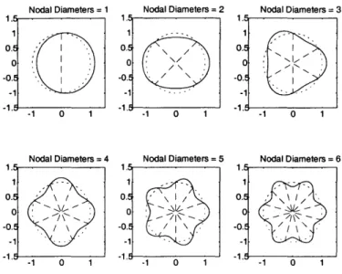
1-1 Two modes of blade vibration, bending and twisting. . . . . 16 1-2 Traveling waves with harmonic number (nodal diameters) 1 through 6. Dotted line is a
reference circle of unit radius. . . . . 17 1-3 Construction of Active Blade: (a) Graphite epoxy skeleton & piezoelectric actuators (b)
Skeleton covered with foam. . . . . 18 1-4 Cross sectional view of active blade. . . . . 18 1-5 Two modes of actuation on a finite element model of the twin spars superimposed on the
original undeformed shape. (a) bending, (b) twisting. . . . 19 1-6 Active Rotor development. (a) Stages for development of rotor, (b) Stages for development
of active blade. Items in the dashed box are testing items that require a sping-testing facility. . . . 22
2-1 Schematic detailing active spar construction. . . . 28 2-2 Experimental setup for system identification. . . . 32 2-3 Transfer function contaminated by the capacitive effect. Notice the slope of the
derever-berant transfer function is 20dB/decade = 1 order of magnitude/decade. . . . 33 2-4 Measured transfer function from command signal applied at leading edge piezos to root
strain at leading edge. . . . 36 2-5 Measured transfer function from command signal applied at leading edge to tip deflection
at leading and trailing edges. . . . . 37 2-6 Cascade of dynamical systems. Note that loading effects between the structure and
actu-ator are indicated by a two way arrow. . . . 42 2-7 First nine modes of twin spar system. Notice that the system acts to a large extent as a
pair
of
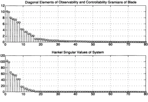
loosely coupled beams. . . . 44 2-8 Coordinate setup for piezo actuation. . . . 45 2-9 Audio amplifier characteristics: Measured response and a second order fit. . . . . 522-10 Diagonal elements of Wc and W and the Hankel Singular Values for the 80 modes of the system . . . . . 2-11 Full order model and reduced order model transfer functions as predicted by FEM based
approach. . . . .
3-1 Basic system block diagram including sensor and process noise. . . . . 3-2 Block diagram of system with process noise adding directly to state vector. . . . . 3-3 Estimator feedback in a dynamical system. The estimator gain matrix uses the error y
-to modify the estimate of system states i. . . . . 3-4 Strain gage noise. . . . . 3-5 Three types of test cases: Pure sinusoidal input, Sinusoindal input with disturbance, No
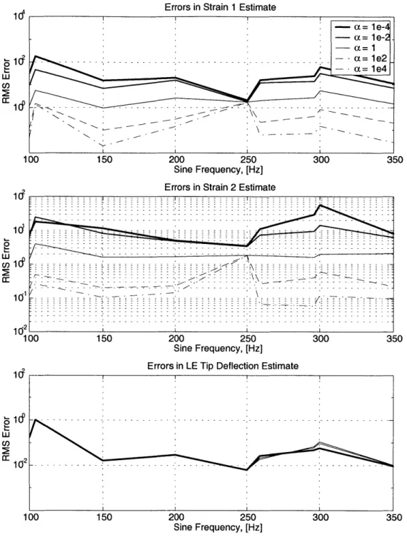
input with disturbance. Disturbances are applied externally and not shown in the plots. 3-6 Variation of errors in estimates with a in response to sinusoidal excitation at various
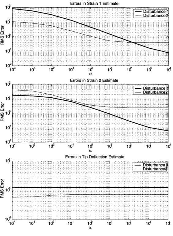
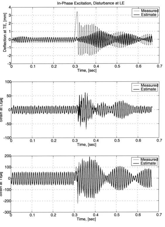
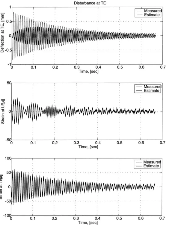
frequencies. . . . . 3-7 Variation of errors in estimates with a in response to a pure disturbance. . . . . 3-8 Comparison between Kalman filter estimate and experiment for a sinusoidal excitation
with disturbance,
a
= 1. Measured and estimate curves coincide in the strain plots. . . . 3-9 Comparison between Kalman filter estimate and experiment for a sinusoidal excitation.a = 1. Measured and estimate curves coincide in the strain plots. . . . . 3-10 Comparison between Kalman filter estimate and experiment for a pure disturbance, a = 1.
Measured and estimate curves coincide in the strain plots. . .
The Spin Test Facility. . . . . Close up view of the main assembly of the Spin Test Facility. Vacuum chamber .. . . . . View from top of vacuum chamber with slip-ring and rotating Exploded view of drive train. . . . . Schematic of vacuum system. . . . . Vacuum system picture. . . . . Main components of oil micro-fog lubrication system. . . . . . Spline shaft notch. . . . . View of lower portion of the rig with sensors installed... Instrumentation readouts and control panel. . . . . Hub and clip concept. . . . .
. . . . 70 . . . 73 . . . . 74 . . . . 75 hub removed. . . . 75 . . . 77 . . . 78 . . . 79 . . . 8 0 . . . 8 1 . . . 82 . . . 83 . . . 84 4-13 Dimensions that were varied in the hub and clip during design stage. . 85 53 53 57 58 58 61 65 66 67 68 69 4-1 4-2 4-3 4-4 4-5 4-6 4-7 4-8 4-9 4-10 4-11 4-12
4-14 4-15 4-16 4-17 4-18
Finite element mesh of one sixth of rotating hub. . . . . Von Mises stresses of rotating hub at full rotational speed (20,000 rpm). . . . . Finite element mesh of one half of clip. . . . .
Von Mises stresses of clip at full rotational speed (20,000 rpm). . . . . Results of thermal test. . . . .
A-1 Measured transfer function from command signal applied at leading edge piezos to strain at root of leading edge (LE). . . . . A-2 Measured transfer function from command signal applied at leading edge piezos to tip
displacement at leading edge (LE) and trailing edge (TE). . . . . A-3 Measured transfer function from command signal applied at trailing edge piezos to strain
at root of trailing edge (TE). . . . . A-4 Measured transfer function from command signal applied at trailing edge peizos to tip
displacement at leading edge (LE) and trailing edge (TE). . . . . A-5 Measured transfer function from command signal applied at both piezos (in phase) to root
strain at leading edge (LE). . . . . A-6 Measured transfer function from command signal applied at both piezos (in phase) to root
strain at trailing edge (TE). . . . . A-7 Measured transfer function from command signal applied at both piezos (in phase) to tip
deflection at leading edge (LE) and trailing edge (TE). . . . . A-8 Inferred transfer function from command signal applied at leading edge piezos to root
.
.
.
.
.
strain at trailing edge (TE). . . . . A-9 Inferred transfer function from command signal applied at trailing edge to r leading edge (LE). . . . . A-10 Transfer function fit to measured data: Input u1, output 61. . . . . A-11 Transfer function fit to measured data: Input ul, output 62. . . . .
A-12 Transfer function fit to measured data: Input u1, output y. . . . . A-13 Transfer function fit to measured data: Input u1, output Y2. . .. .. . . . . A-14 Transfer function fit to measured data: Input u2, output
e1.
. . . . A-15 Transfer function fit to measured data: Input u2, output 62 . . . .. . . . ..A-16 Transfer function fit to measured data: Input u2, output Y1. . . . . A-17 Transfer function fit to measured data: Input u2, output Y2. . . . .
. . . 107 oot strain at . . . 107 . . . 108 . . . 109 . . . 109 . ---- 110 . . . 110 .. ---- 111 . . . 111 . . . 112 88 88 89 89 92 100 101 102 103 104 105 106
List of Tables
1.1 Active Rotor blade summary . . . . 1.2 Flutter frequencies of the Fan C blade . . . .
2.1 Inputs, outputs, and measured data of Active Blade. 2.2 Summary of measured and inferred transfer functions 2.3 Instrumentation setup parameters. . . . .
4.1 Spin Test Facility summary . . . . 4.2 Mechanical properties of selected materials for rotating hub and blade retention clips. 4.3 Parameters of finite element models of hub and clips. . . . .
A.1 Directly measured transfer functions and their figures. . . . . . . 21 . . 21 . . 31 . . 34 . . 35 76 87 87 99
Chapter 1
Introduction
1.1
Aeroelasiticity in Turbomachines
Engine high cycle fatigue (HCF) is one of the main factors limiting the development of more powerful, lighter, and higher performance gas turbine engines. Vibration of rotating bladed structures has been a main concern for designers since the inception of gas turbines for power generation or aeropropulsion. One of the causes of vibration in turbomachines is the dynamic coupling between structural and aerodynamic forces in an engine. Under certain conditions, vibration in a bladed structure rotating in a high energy flow leads to pressure perturbations in the fluid. These pressure perturbations can feedback in a positive sense into the vibration of the structure. In effect, the fluid will be providing negative damping to the structure, thereby doing work that increases its vibration levels, leading to overall system instability. This mode of instability, known as flutter, may lead to mechanical failure of the blade, or to sustained high levels of vibration and dynamic stresses, which in turn reduce the fatigue life of the structure.
Flutter may occur in situations where a vibrating structure is exposed to a fluid flow. A structure, such as an aircraft wing, may experience flutter as it vibrates in a flow of air. In turbomachines, the problem is generally much more complex than in isolated structures [8]. In the case of a solitary structure, the fluid forcing function is solely due to its own motion. However, in blade cascades in turbomachines, the forcing function on a blade is due to its own motion, as well as the motion of other blades in the cascade. Specifically, it depends on:
* Mode shape of vibration of individual blades. Typically the mode shapes are of bending or twisting,
" Temporal variation of motion of blades. Assuming that all blades vibrate with the same mode
shape, they do necessarily do so in unison. The temporal variation of motion is captured by
traveling waves along the circumference of the rotor. Traveling waves are characterized by a harmonic number, or number of nodal diameters, as shown in figure 1-2.
" Interblade phase angle, which is the phase relationship between the motion of a blade to other blades.
,ZIEAIE
Figure 1-1: Two modes of blade vibration, bending and twisting.
This introduces a grid of interactions with several dimensions: interblade phase angle, harmonic number of traveling wave mode, and vibratory modes of individual blades. As a result, the complexity of the problem is significantly higher than the case of a solitary structure.
Current state-of-the-art design tools fail to adequately account for flutter in the early design stages of engines. This is primarily due to the lack of flutter prediction models, which in turn is due to a lack of experimental data in that area. In order to validate any proposed model for flutter prediction, there is a need for reliable experimental data. The lack of experimental data in aeromechanics is a result of the difficulty and cost associated with conducting reliable experiments. This is largely due to the harshness of the operating environment, as well as the difficulty in controlling a flutter instability once it occurs.
For a complete and detailed treatment of aeroelasticity and forced vibration in blade cascades, refer to [8] and [21].
Nodal Diameters = 1 1. 0. 1 0 -0.. 1 -1.0 -1 0 1 Nodal Diameters = 4 1. 0.5 0 -0. -1 -1.0 - 0 1 Nodal Diameters 2 10. 0 \0 / -0. / ' -1 -1 0 1 Nodal Diameters 5 1. 0. '. 0 -0. 1 -1 --1. 1 0 1 Nodal Diameters = 3 1. 0. 1 0 -0.! -1 1. -1 0 1 Nodal Diameters 6 1.5 1 0 -0. , -1 -1.L -1 01
Figure 1-2: Traveling waves with harmonic number (nodal reference circle of unit radius.
diameters) 1 through 6. Dotted line is a
1.2
The Active Rotor
The Active Rotor is a proposed tool for conducting experimental investigations of flutter in blade cas-cades. Essentially it is a rotor in which the motion of individual blades are actuated and controlled. The two basic modes of actuation considered are bending and twisting, replicating the two fundamental flutter modes in most blades. In this section, the actuation concept is described. The need for the active rotor is then motivated through a description of three potential experiments that would require such a device. Finally a description of the rotor, its geometry, features and functional requirements is presented.
1.2.1
Concept
The currently adopted concept for the Active Rotor is what is dubbed the "spar-and-shell" concept. Because the energy required to actuate a typical steel or titanium blade is very high, alternate blade materials are used. Consider a pair of graphite-epoxy spars as shown in figure 1-3(a). Piezoelectric laminates (PZT-5A') are bonded to the root of the spars on each face. By applying suitable potential to these laminates with correct polarity, each spar can be independently deflected. Actuation of the spars
in-phase will create an overall bending deformation of the structure, whereas actuation out-of-phase will create a twisting deformation. The two modes of actuation are illustrated in figure 1-5. Sensing is attained through the use of strain gages bonded on the exposed surfaces of the piezos, thereby providing collocated actuation and sensing. The aerodynamic shape is obtained by covering the twin-spar set with high strength-to-weight ratio foam2 that is shaped and bonded to the skeleton.
Spars Piezo-Actuator Blade Root (a)
Figure 1-3: Construction of Active Blade: (a) Skeleton covered with foam.
Foam
(b)
Graphite epoxy skeleton & piezoelectric actuators (b)
Piezo-Actuators
LE
1.2.2 Motivation
In order to motivate the utility of the Active Rotor, three potential experiments are described that will test for different aspects of flutter. These experiments either necessitate such an experimental device, or are conducted with the active rotor with significant simplicity and reduction of costs. Experiments 1
(a)
(b)
Figure 1-5: Two modes of actuation on a finite element model of the twin spars superimposed on the original undeformed shape. (a) bending, (b) twisting.
and 2 focus on determining the dynamical characteristics of the rotor, and may be regarded as different approaches to the same test, whereas experiment 3 studies the effects of mistuning in rotors.
Experiment 1: Measurement of Influence Coefficients: The effect of the motion of one blade on another is captured by influence coefficients. In general, the motion of a blade will cause pressure perturbations on other blades. The nature of these perturbations depends on the mode shape of one blade vibration, the harmonic mode number of the traveling wave of blade vibrations, the interblade phase angle, as well as the flow conditions. Generally, if the equation of motion of a blade is written in modal coordinates, the single DOF equation of motion for a particular mode is:
mi'e + bitb + kiw = Ai(11
where mi, bi, ki and
fi
are the modal mass, damping, stiffness and generalized forcing function for blade mode i. The forcefi
is a summation of contributions of the effects of the motions of all the blades in the cascade, and is given by 1.2:N-1
it = 2 0 EZ CoOiej(wt+iO) (1.2)
where 0, is a blade vibration mode, with an amplitude determined by the travelling wave mode qo and phase 0. Co is a complex influence coefficient that relates the force generated on the blade due to the motion of another at interblade phase angle n for the given modes. Proper dimensions are obtained by multiplying by the dynamic pressure 2V1
l
0, where p is the fluid density, V is the mean flow velocity and 1, is the blade chord length.Using the Active Rotor, the motion of some blades may be prescribed and controlled, whereas the motion of other blades are passively measured. From the measured deflection of the passive blades, the generalized forcing function
fi
may be backed out. Using equation 1.2, and knowing all the prescribed motions of the other blades, the influence coefficients Co may be calculated.Experiment 2: System Identification Based Approach: The system identification based ap-proach is more focused on investigating the effect of the aeroelastic coupling on the overall damping of the system. Using regular systems identification techniques (e.g. measuring response due to sine sweeps), the modal characteristics of a system may be obtained in terms of natural frequencies and damping ratios. To eliminate the effect of aerodynamics, the system may be identified in vacuum, and the modal parameters obtained. The experiment may be repeated in the presence of flow, and new damping ratios may be calculated. A decrement to the damping ratio would indicated a system where the fluid is doing work on the structure.
This experimental approach may also be used to verify some of the basic assumptions of current state-of-the-art flutter analysis. One example is the assumption that the aerodynamics affect the damping ratios of the structure, but leaves the natural frequencies largely unaffected [8].
Experiment 3: Investigation of Effect of Mistuning Parameters Mistuning is the variation of natural frequencies and mode shapes of individual blades in a rotor. Mistuning may be a result of slight material and manufacturing tolerances of the blades, or it may be intentionally induced in a rotor as a means of passive flutter control [8]. Mistuning of blades can either have desirable or adverse effects on the structure. Under some conditions, mistuning may result in the localization of energy on a single blade. In other cases mistuning may plateau sharp resonance peaks in a structure to milder levels. The experimental study of the effect of mistuning parameters on the structural response is generally costly since it requires the building of different rotors. Investigation of mistuning in blade stiffness has been a more common approach. Such studies may be implemented in the Active Rotor by applying feedback control to the piezo actuators to provide controlled changes in stiffness and natural frequencies of individual blades. Alternatively, geometric mistuning may also be studied since altering the angle of twist of individual blades becomes possible.
1.2.3
Features and Functional Requirements
The geometry of the Active Rotor is matched to that of the rotor studied in [16]. A summary of the basic features of this rotor is outlined in table 1.1. This is 33 % dynamically reduced version of the General Electric Fan C design, and is known to exhibit flutter problems as described by table 1.2. Thus, the selected geometry is an interesting one from a flutter standpoint, and will allow bench-mark comparisons with.the results in [16]. For notational purposes, the selected geometry will be referred to as the "scaled
Fan C".
Property Value
No. of stages 1
Tip diameter 53.14 [m]
Hub/tip radius 0.36
Tip Mach speet 1.52
Rotational speet 16,700 [rpm]
Chord length (at root) 6.36 [cm]
Chord length (at tip) 8.92 [cm]
Max. thickness to camber ratio (at root) 0.114 Max. thickness to camber ratio (at tip) 0.027
Stagger (at root) 6.47 [degrees]
Stagger (at tip) 71.11 [degrees]
Camber (at root) 91.10 [degrees]
Camber (at tip) -1.664 [degrees]
Solidity (at root) 2.414
Solidity (at tip) 1.389
Table 1.1: Active Rotor blade summary
Table 1.2 shows the flutter frequencies of the scaled Fan C blade. They suggest that the actuation bandwidth of the active rotor should be in the 1 kHz band to cover both torsional and bending flutter. A reduced bandwidth of ~350 Hz may be sufficient for the study of bending flutter only.
Operating Speed [% of Nominal] Flutter Mode Flutter Frequency [Hz]
65 Torsional 896
70 Torsional 896
90 Bending 320
95 Bending 336
From a conceptual design standpoint, the amplitude of actuation is selected to be 1 degree of tip twist, and correspondingly ~1.0 mm of tip displacement in bending at the spar tips. This requirement however may turn out to be superfluous. Experimental investigations in [12] and numerical simulations in [23] have shown that an angle of twist of 0.3 degrees are sufficient creating measureable aerodynamic responses.
1.3
Development Stages of an Active Compressor Blade
The development of the Active Rotor can be grouped into four general areas of work. They are shown schematically in figure 1-6, and outlined below:
Active blade
---development Blade design, Testing for analysis and structural integrity manufacture
Integration of multiple
blades into a complete Characterization of Testing for rotor blade dynamics actuation capability
Shakedown at MIT
Blowdown compressor Dynamics, Testing of estimation and 7 performance
control Off-site
experimentation for flutter testing.
(a) (b)
Figure 1-6: Active Rotor development. (a) Stages for development of rotor, (b) Stages for development of active blade. Items in the dashed box are testing items that require a sping-testing facility.
Active Blade Development
The development of an active blade is indeed the core task towards the development of a complete rotor, and perhaps the most challenging. Major issues include:
Design, Analysis, and Manufacture of Active Compressor Blade: Design of the blade must ensure the capacity to sustain centrifugal loads. Finite element models were developed to aid
in the design process, and studies were perfomed on the optimal lay-up patterns of graphite epoxy. Coupon tests for establishing the feasibility of the actuation concept were conducted, as well as studies for actuator selection and sizing. These key issues in the design and analysis of the blade are outlined
in detail in [14].
The complex bilinear curve and twist in the blade geometry adds challenges to the manufacturing processes. Several manufacturing options are considered. Until the writing of this thesis, no final conclusions have been set on the optimal method of blade manufacture. Although a pair of active spars were successfully developed and used for initial experimentation, as yet a complete blade with properly shaped foam is still under development.
Dynamical Characterization: The central functional requirement of the active rotor is the ability of its blades to follow prescribed deflection trajectories. In order to develop suitable control laws, the dynamics of the blade (the plant) must be carefully modeled. A model is useful only if validated experimentally, and proven to predict the response of the system in hand. This dictates the necessity to
conduct experiments for validation and tuning purposes.
The main parameters of interest in the deformation of the blade are the tip deflections: pitch and plunge. Chord-wise deflections are neglected, and assumed not to contribute significantly to aeroelasitic effects.
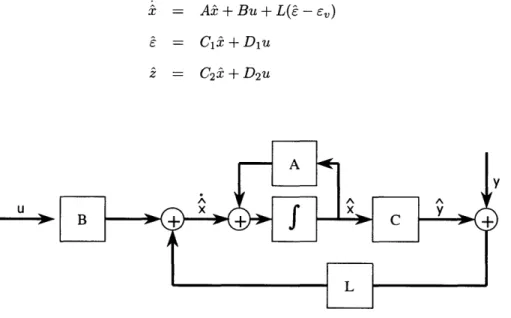
Development of Control and Estimation Laws: Once a suitable dynamical model for the blade is developed and verified, control algorithms are required to command the blade to specified trajectories. Recall that actuation is provided by piezos, while sensing is attained by collocated strain gages. A state estimator is needed for estimating blade tip deflection (parameters of interest) given strain readings at the root. This will serve as an alternative to direct measurement of tip deflection, which is typically difficult. Furthermore, development of state estimators is a prerequisite to the development of state feedback controllers.
Development of a Spin-Testing Facility: Figure 1-6 shows that spin testing is required through-out the development stages of the rotor. This necessitates the development of a high speed spin-testing facility that will fulfill such testing needs. The spin-test facility must be capable of providing evacuated environments to isolate structural and aeroelastic dynamics. Although this facility was developed with the active rotor in mind, it may be used in its own right as a general spin-testing facility for other purposes.
Integration of Multiple Blades Into a Complete Rotor
Once a reliable procedure for the development of an active blade is set, multiple blades may be reproduced and integrated into a complete rotor. Issues to be considered at this stage include the design of a suitable rotating hub to accommodate the cascade, and the proper wiring of sensors and actuators. Due to the limited number of channels available for communication with the rotor in a rotating frame of reference, some ideas have been suggested with regard to on board multiplexing of the signals to provide an expansion of the communication channels.
Shakedown in the MIT Blowdown Compressor
Shakedown is to be performed in the MIT blowdown compressor, where the rotor is briefly exposed to aerodynamic loading. This step is necessary to ensure that the rotor will survive aerodynamic loading.
Off-site Experimentation
Full off-site experimentation for flutter will require more extensive facilities. Suggested locations include
NASA Glenn Research Center or Wright-Patterson facilities. Upon arriving at this stage, the experiments
outlined in section 1.2.2 may be conducted.
1.4
Organization
This thesis is part of the effort towards the development of an active blade. Specifically, it focuses on three aspects:
o Chapter 2 focuses on the dynamical characterization of the active blades and obtaining models suitable for estimation and control. Two approaches are presented, with the advantages and disadvantages of each are discussed. Since active blades are under development, the procedures are implemented on the active structure of the blade, the twin spar system, which was available at the time. The first approach is a purely empirical approach in which the transfer functions of the blades are empirically determined. The experimental setup is described, and results are presented. Transfer functions are then fit to the data in a least squares sense. Model order reduction using Hankel Singular Values is presented and implemented, resulting in a model of reasonable order from an implementation perspective. The second approach depends on finite element modeling of the blade to obtain its dynamical characteristics. The model order is reduced, and the actuation effects of the piezos is modeled, and the dynamics of supporting signal conditioning amplifiers are identified experimentally, and fit to a second order system. The results of this approach were then
compared to experimental results. Appendix A compliments this chapter, and documents all the transfer functions measured and fit.
" Chapter 3 discusses the design of state estimators for estimating blade tip deflection from root strain gage measurements. Such estimates are required since direct measurement of tip deflection for a complete rotor is experimentally infeasible. Kalman filters are demonstrated via simulation. The estimates are compared to experimental data.
" Chapter 4 discusses the development of a Spin Testing Facility for testing of active blade. The Chapter discusses the functional requirements, and relates them to the sub-systems and compo-nents of the facility. The design of a rotating hub to accommodate candidate blade concepts for testing is presented, including results of finite element simulation for stress analysis under centrifu-gal loading. Instrumentation for rig condition monitoring is outlined. Precautionary measures with regard to rig assembly are presented based on experience gained during the development of the rig. Finally, results pertaining to thermal characterization of the rig to determine safe operation durations is presented.
Chapter
2
Dynamical Characterization of an
Active Compressor Blade
The central functional requirement of the Active Rotor is the ability to dynamically deform its blades according to prescribed trajectories. To do so, piezoelectric actuators apply strain loading at the root of the blade, whereas strain gages provide collocated sensing. Before being able to make use out of the active structure, its dynamics must be studied and understood. This chapter focuses on a procedure for dynamical characterization of an active blade, and obtaining low order models that characterize the behavior of the Active Blade.
Due to the bilinear curvature, twist and taper of the blade geometry, analytical modeling is infeasible. Instead, two alternate approaches are presented. The first approach, as outlined in section 2.1, is a purely experimental approach in which the transfer functions are empirically determined. The second approach relys on a combination of finite element modeling and experimental results to arrive at a dynamical model of the blade and its supporting signal conditioning systems. This is outlined in section 2.2. Each approach has its advantages and disadvantages, and will be discussed in the sections that follow.
The goal of Chapter 3 is to design state observers for the blade, to estimate its deflection state given root strain gage readings. The parameters of interest from an aeroelasticity perspective are the two degrees of freedom of tip deflection: pitch and plunge. Obtaining a dynamical model for the blade is essential to design of model-based state estimators. Furthermore, the models generated will serve as a basis for designing controllers that will command the blade to move according to desired trajectories.
complete Active Blade has not been completed'. Instead, a pair of curved, twisted, fully packaged and wired active spars are available without any foam. This structure is used as the test article for the studies presented here and in Chapter 3. The results will vary significantly with the addition of foam since it will alter the dynamical characteristics of the system under consideration. The foam will not only add mass, stiffness and hysteretic damping to the structure, but it will also couple the two spars together, which was not the case considered here. Nevertheless, developing the identification and estimation procedures at this early stage provides useful information that will be applicable to the full blade. Therefore the purpose of this chapter and of chapter 3 is to develop characterization and state estimation procedures that are applicable to the twin spar set, with the intention that such procedures will be replicated when the Active Blade is complete.
Description of Active Spars
Before getting into the identification procedures, it is worthwhile at this stage to give a detailed descrip-tion of the system under consideradescrip-tion. Figure 2-1 shows the construcdescrip-tion of an active spar. Recall that a single blade will have two of such spars, one close to the leading edge, and another close to the trailing edge. Additionally, the two spars do not have identical geometries as illustrated in figure 1-3(a).
Suction Side
Pri gStrain gag
( Pinaien own
Trailing edge Gietlodwn spar Leading edge spar Epoxy layers
r
Indicate piezo orientation Tapered sparPiezo Strain gage
Pressure Side (orientation up)
oopelkepton
vpiezO
Blade root
Figure 2-1: Schematic detailing active spar construction.
Epoxy layers bond the inner surfaces of the piezo actuators to the spars, and the strain gages to the outer surfaces of the piezos. A potential difference is applied across the inner and outer surfaces.
1The scope of this thesis does not include the development nor manufacture of the Active Blade.
Because the piezos are oriented in opposite directions (as indicated by the arrows), they work together producing maximum structure deflection. Had the piezos been oriented in the same sense, they would work against each other, producing zero net effect.
Modes of Actuation
The two basic modes of actuation of the blade are bending and twisting. A simple approximate way to achieve these modes is to provide both the leading and trailing edge piezos a common potential for bending, and opposite potentials for twisting. However, since the two spars have slightly different geometries, the phase difference from voltage applied on actuators to tip deflection is not necessarily the same for both spars. Therefore the structure is regarded as a multi-input, multi-output (MIMO) system in which the effect of each input is analyzed separately.
Model Bandwidth Requirements
Table 1.2 shows that the maximum flutter frequency of the active rotor under consideration is 896 Hz. Consequently, the bandwidth requirement set for the rotor is 1 kHz. However, it is also evident from the table that a bandwidth of 400 Hz would be sufficient to address the bending flutter problem. These figures dictate the bandwidth of validity of the dynamical models to be obtained, which depends on the flutter mode studied. As will be shown in section 2.1.1, the experimental approach to determining system transfer functions requires laser vibrometers to measure blade tip displacement. The available vibrometers are limited to a bandwidth of 400 Hz. Therefore, all models obtained by that method can be used to investigate only the bending flutter problem. Higher bandwidths would require the use of the higher bandwidth instrumentation that are not currently available. Alternatively, the second approach, the finite element approach, may be used to yield models that are valid up to higher frequencies.
Comparison of Two Modeling Approaches
The experimental approach to system identification relys on exciting the structure with broadband input up to the desired bandwidth, and measuring the transfer functions from all inputs to all outputs. The inputs in this system are command signal voltages that are amplified and applied to the piezo actuators. The outputs are strain gage readings and tip displacement measurements. This approach has several advantages:
" Directly captures the dynamics of the structure under investigation.
" Accounts for the dynamics of actuators, amplifiers and signal conditioning equipment since they are lumped with the system being identified.
* Captures imperfections in the system that are otherwise hard to model, e.g. imperfections of bonding of actuators or sensors to the structure.
The disadvantages of the experimental approach include:
" Resulting model bandwidth is limited by instrumentation bandwidth.
" No insight is obtained on how the response of the system will vary by changing some of its features. For each system, a new set of experiments must be conducted.
" The method can only be implemented easily on a bench top test. Identification under rotation would require special blade tip deflection measurement instrumentation.
On the other hand, the finite element model based approach relys on obtaining the dynamical char-acteristics (natural frequencies and mode shapes) from a finite element model. This information is then augmented by models of amplifiers and signal conditioning equipment. Finally, the entire setup is put in state space form. The resulting model, having a large order due to the nature of finite element modeling, is then approximated by a reduced order model. This approach, though being more involved and less direct than the first one, has several advantages:
" Obtains estimates for system response beyond bandwidth limitations of sensors.
" Predicts model response at all points of structure, as opposed to only points of measurement of strain at roots and displacement at tip.
" Provides for the analysis of the effects of structural modification. Since the active blade is under development, modifications are prone to happen. For example, the leading and trailing edges may need strengthening by adding fiberglass lining. Such modifications may be included in the FEM model, the effect of which may be simulated and predicted.
" Allows for investigation of gains and losses in observability and controllability of the system due to addition/removal of sensors/actuators. For example, consider a situation when an added strain gage is to be placed on the blade to obtain more accurate sensing of the deformation. Optimal locations for the sensors may be chosen on the model to yield maximum gain in observability.
* Predicts model tip response under centrifugal loads. Centrifugal stiffening effects alter the dynamics of the system, the effect of which can be studied through the model.
The main disadvantage of this approach is that tuning the finite element model to match actual system characteristics may be cumbersome, and results may be inaccurate. Careful modeling of boundary
condition and material properties is essential. Furthermore the presence of manufacturing imperfections are hard to capture.
In the sections to follow, each approach is presented in more detail, and the results are compared. As will be seen, the two results do not match to a certain extent, and possible remedies are discussed.
2.1
Experimental Determination of Transfer Functions
The experimental approach to characterizing system dynamics depends on exciting the structure with broad band excitation and measuring the response at select points. For the twin spars, there are two inputs and six output sensors as explained by table 2.12. Strain gages si and 83 are on opposite sides of the leading edge spar, and therefore measure the same strain, but with opposite signs (1800 phase shift).
Thus an average value for the strain at the leading edge is obtained by
E,
=}(s
- 83). Similarly, the same calculation is applied to E2, the average strain value at the root of the trailing edge. In summary, the system has two inputs (ui and u2), and four outputs (E, 62, z1, z2), which are determined by six sensors (si, s2, 83, 84, zi, z2).Quantity Designation Transducer/Actuator
Actuation at LE U1 Piezo actuator
Actuation at TE U2 Piezo actuator
Root strain at LE suction side si Strain gage
Root strain at LE pressure side S2 Strain gage
Root strain at TE suction side S3 Strain gage
Root strain at TE pressure side S4 Strain gage
Average root strain at LE 61 =
4(si
- 83) Calculated Average root strain at TE 62 = 2(82 - 84) CalculatedTip displacement at LE z Laser displacement vibrometer
Tip displacement at TE Z2 Laser displacement vibrometer
Table 2.1: Inputs, outputs, and measured data of Active Blade.
2.1.1 Experimental Setup
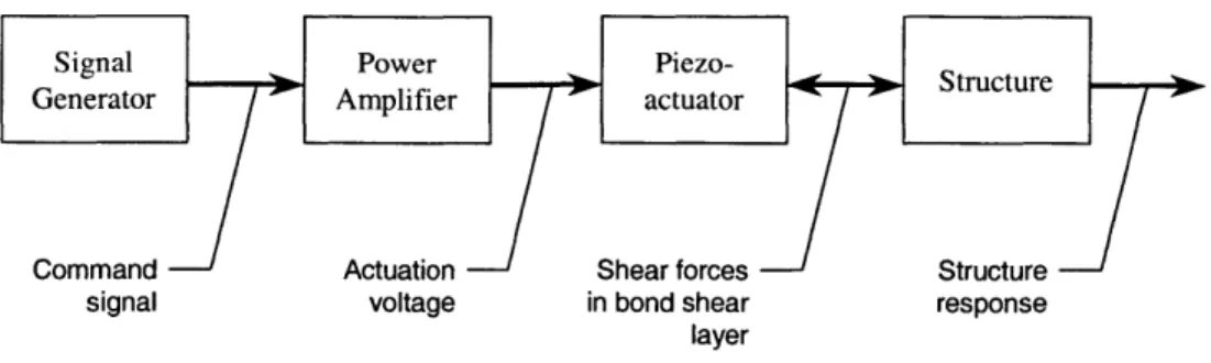
Figure 2-2 shows the setup used to run system identification experiments. A signal generator provides an excitation sinusoidal sweep command signal. This signal is amplified via an audio power amplifier,
and its voltage is further raised by transformers. The piezo actuators excite the structure which in turn deforms. Strain gages measure the root strain and a laser displacement transducer measures tip deflections. Strain gage amplifiers implement a Wheatstone bridge circuit to accurately measure the small changes in resistance associated with the deformation of the strain gages. The frequency response of each of the outputs due to the input signal is computed by a dynamic signal analyzer. The analyzer averages out sample response until a suitable coherence spectrum is achieved.
Test Article Piezo Voltag -- -Strain Gage Amplifiers 0000 _,0000 00003 000 Spectrum Analyzer (replaced with DAQ system for
time domain measurements)
Command Sign
e
Transformer + DC Offset Voltage Supply
2 Channel
Power Amplifier
Signal Generator al
Figure 2-2: Experimental setup for system identification.
It is important to emphasize that the "command signal" is that generated by the function generator (on the order of 1 Vpp), whereas the "piezo voltage" is that applied on the piezo, or the amplified version of the command signal (on the order of 250 Vp,,). Transfer functions are obtained with respect to the command signal as input to the system. This is done to take into account the dynamics of the amplifier, and have it included in the system response. Furthermore, from a controller implementation point of view, the output of the controller will be that command signal, and therefore should be taken as input to the plant.
Laser Vibrometer
Capacitive Effect of Epoxy Layers
The correct choice of which piezo leads to ground is very important. Figure 2-1 shows that the outer surfaces of the piezos are grounded. If the converse is true, then the upper surfaces would experience a fluctuating potential on the order of 250 Vp,, while the strain gages will remain at a virtually constant potential. This creates a situation where two conductors (the outer piezo surface and the strain gage) are at a potential difference, separated by a dielectric layer (epoxy). This, by definition, is a capacitor, the presence of which highly contaminates strain gage readings. Figure 2-3 shows a sample transfer function obtained with the presence of such capacitive effect. Two things are immediately noticed: i) the dereverberant part of the transfer function3 is increasing at a slope of +20dB/decade, and ii) the poles and zeros are highly attenuated. These trends can be explained by the presence of this capacitive effect which introduces a differentiation element, and hence a 20 dB/decade slope. The most effective way to eliminate such effects is to ground the outer surfaces of the piezos, and thereby eliminating the potential difference, and the entire capacitive effect.
Transfer Function from Command Signal to Root Strain. Input to Piezos in In-Phase.
.5 102 2 1 -10 10, 102 103 0 Frequency Hz -- - - - - - - - - - - - - --100 --- - - - - - - - - - --I- _ _ _ _ _ _ - _ _-a C. C -150 --- - - --200 10 102 10 1 Frequency, Hz 0.5 - - - - - - - - - - - -01 10 102 103 Frequency, Hz
Figure 2-3: Transfer function contaminated by the capacitive effect. Notice the slope of the dereverberant transfer function is 20dB/decade = 1 order of magnitude/decade.
3
The twin spar test article available at the time of testing did not allow for complete freedom of choice of which leads to ground. This is because a common connection is hardwired to the inner surfaces of the four piezo. Thus it is not possible to excite both the leading edge actuators and the trailing edge actuators with different signals simultaneously. Consequently not all transfer functions could be measured directly, and some had to be inferred from the other results. Table 2.2 outlines:
Out put\Input U1 u2 U1 + U2 U1 - U2
LE Actuation Only TE Actuation Only In-Phase Acutation Out-of-Phase Actuation
61 Measured Inferred Measured Inferred
62 Inferred Measured Measured Inferred
E3 Measured Inferred Measured Inferred
64 Inferred Measured Measured Inferred
zi Measured Measured Measured Inferred
Z2 Measured Measured Measured Inferred
Table 2.2: Summary of measured and inferred transfer functions
Important Considerations
The experimental setup in hand involves large actuation voltages, and sensing voltages on the order of millivolts, all packaged in a very compact space. To aggravate the situation further, the electric motor of the Spin Test Facility produces a significant electromagnetic field that may easily cause interference with the measured signals. Thus great care in setting up the electrical connections is essential to obtain good quality results. The following is a highlight of some good practices that must be followed:
" Electrical grounds of the piezo actuators and strain gages should remain isolated. During the course of experimentation, the potential of the two grounds may change, and the presence of a conductor with a small but finite resistance will cause ground loops that contaminate the readings of the strain gages.
* Outer sides of the piezos must be electrically grounded to eliminate the capacitive effects mentioned above.
* All wires leading to strain gages must be paired and twisted to eliminate electromagnetic interfer-ence.
* All wires in the rotor must be shielded, especially those leaving the slip ring and are subject to interference patterns due to the operation of the motor.
Equipment Setup
To excite the structure and measure its response, the equipment were set as described by table 2.3:
Instrument Parameter Setting
Function Generator Mode of operation Sine sweep Frequency range 50 Hz to 1200 Hz
Amplitude 1 VP,
Sweep time 4 seconds
Sweep mode Logarithmic
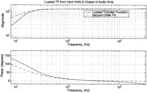
Audio Amplifier Mode 2 channel, stereo
Gain setting Maximum
High pass filter 40 Hz
Strain Gage Amplifier Bridge mode Quarter bridge
Active filter 10 kHz, low pass
Gain 300 pe/V
Laser Vibrometer Gain 1,623 pm/V
Mode Fast response
Spectrum Analyzer Mode 2 Channel
Measured data Frequency response
Coherence spectrum
Window mode Hanning
Frequency range 1.6 kHz Frequency resolution 800 lines
Averaging 200 averages
Channel setup Grounded, auto-range
Table 2.3: Instrumentation setup parameters.
Since the signal analyzer available is a two channel analyzer, experiments were conducted in sequence, measuring one SISO transfer function at a time in accordance with table 2.2. Data are then transferred from the analyzer for further processing.
2.1.2 Results
All measured transfer functions are plotted in Appendix A. Only two are presented here to aid in the discussion. Figure 2-4 shows a plot of the transfer function between a command signal applied to the leading edge actuators and root strain at the leading edge for a frequency range from 0 to 1,200 Hz. The following observatoions are made:
* Two poles dominate the response at frequencies of 114 Hz and 322 Hz, while other less obvious poles are at approximately 279 Hz, 640 Hz and 710 Hz. Zeros cancel the poles at frequencies of 124 Hz, 293 Hz, 342 Hz, 645 Hz and 732 Hz. Thus, poles and zeros of the system interlace in a manner as expected in collocated actuation and sensing [4].
Transfer Function from Command Signal to Root Strain. Input at LE Piezos. E a) 0 10 3 10 2 10 1 10 0 200 150 100 50 0 -50 -100 -150 -200 0.8 0.6 0.4 0.2 0 200 400 600 Frequency, Hz 800 1000 1200
Figure 2-4: Measured transfer strain at leading edge.
function from command signal applied at leading edge piezos to root
" The dereverberant transfer function is fairly constant over the entire frequency range. This is
an expected trend in structures where the input is a strain actuator, and the measured output is also strain. Different actuator/sensor combinations yield different roll-off frequencies of the dereverberant transfer function.
" The phase difference between the suction side strain gage and the pressure side strain gage is an
almost constant 1800. This is expected when measuring strain at two different sides of a cantilever beam. Imperfections are attributed to the twist and curvature in spar shape, as well as to the fact that strain gages are located at slightly different positions axially with respect to the spar base.
" Coherence is a measure of the quality of correlations obtained. Values are almost perfect for the
entire frequency range, with the exception at zero locations. This is because the response is very small at those locations, making the signal to noise ratio small.
0 200 400 600 800 1000 120C Frequency, Hz E-0 0 0 200 400 600 800 1000 120 Frequency, Hz
-H
- - - - -- - - --- - --- --- ---- ----- --- -------
---
----
- - - - - ---- ---- --- - - --- - - --- - - - - --- - - -- - ---- -- --- - -- --- - ---- -- -- - -- --- - -- -- - ----- --- -- - - -- - -- - - - - --~-
- - -- - - ---- ---- ---- --- -- -L0
Z Z - - -- - -- - -- - - - - - - - - - - - - - - -- - --- - - - - LE SuctionLE Pressure -- - - -- - - - -- - - - - -- -- -- -- -- -- -- -- -- -- -- -- -- -- -- -- - - - --- - - - - - -- -- - - - - -- -- -- -- -- - - - -- - - - - -_ _ - - - - - - - - --- - - - -- -- -- -- -- -- - - - - -- - - - --- - - --- - - -- - - - --Z --Z Z - - - --- - - --- - - -- - - - --- --- --- --- --- --- --- --- --- --- --- --- --- --- --- --- --- --- --- --- --- - - - - - - - - - - - - --- --- --- --- --- --- --- --- --- --- - - - -0 - - - -- - - ---
--- -- ---Figure 2-5 shows the transfer functions from a command signal applied to the leading edge actuators to tip deflection of the leading and trailing edge spars.
6 ac to L> 10 1 10 0 10 -1 10 -10
~
10 -4 200 150 100 50 0 -50 -100 -150 -200 0.8 0.6 0.4 0.2 0Transfer Function from Cornmand Signal to Tip Deflection. Input at LE Piezos.
-
~
~~
- - - - - - - - - - - - - - - - - - --LipD f cin - - - - - - - - TE Tip Deflection-- -p- -- \ -------- -- --200 400 600 800 1000 12( Frequency, Hz - - --- - - - - - - - - --- .. - - - - - r ---- -- - - - - - - - - - - -- -- -- --- - - - - - - - - - - - - - - - - - - - - - -200 400 600 800 1000 120( Frequency, Hz S- -- - - - - - - - - - - -- -- -- -- I --1 --,Jl I -. I - - - -I - - - - --- I - --- - --- - --I JI -- - - - - - - - --- - - - - -9 - - - -~rIA 1 *~ 0 200 400 600 Frequency, Hz 800 1000 1200Figure 2-5: Measured transfer function from command signal applied at leading edge to tip deflection at leading and trailing edges.
" Notice the sharp drop in coherence levels at the 400 Hz cut-off mark. This is the bandwidth of the laser displacement vibrometer, and will be the frequency range considered.
* As with figure 2-4, there are two dominant poles in the response of the system at 105 Hz and 296 Hz. Poles and zeros are not as closely spaced as in the case of figure 2-4 because actuation and sensing are not collocated.
* The response of the leading edge tip is larger than that of the trailing edge. This is because the coupling between the two spars is small. The presence of foam is expected to increase the coupling significantly, and thereby increasing the response of the trailing edge to level comparable with those of the leading edge.