Dynamic valuation model For wind development in regard to land value, proximity to transmission lines, and capacity factor

Dynamic Valuation Model For Wind Development In Regard to Land Value, Proximity to Transmission Lines, and Capacity Factor

by

Paul Nikandrou

SUBMITTED TO THE DEPARTMENT OF MECHANICAL ENGINEERING IN PARTIAL FULFILLMENT OF THE REQUIREMENTS FOR THE DEGREE OF

BACHELOR OF SCIENCE IN ENGINEERING AS

RECOMMENDED BY THE DEPARTMENT OF MECHANICAL ENGINEERING AT THE

MASSACHUSETTS INSTITUTE OF TECHNOLOGY MAY 2009

© 2009 Massachusetts Institute of Technology. All rights reserved. The author hereby grants to MIT permission to reproduce and to distribute publicly paper and electronic copies of this thesis document in whole or in part in

any medium now known or hereafter created.

Signature of Author: ________________________________________________ Department of Mechanical Engineering

May 8, 2009 Certified by: ______________________________________________________

Alexander H. Slocum Professor of Mechanical Engineering, MacVicar Fellow Thesis Supervisor Accepted by: _____________________________________________________

John J. Lienhard V Collins Professor of Mechanical Engineering Chairman, Undergraduate Thesis Committee

Dynamic Valuation Model For Wind Development In Regard to Land Value, Proximity to Transmission Lines, and Capacity Factor

by

Paul Nikandrou

SUBMITTED TO THE DEPARTMENT OF MECHANICAL ENGINEERING IN PARTIAL FULFILLMENT OF THE REQUIREMENTS FOR THE DEGREE OF

BACHELOR OF SCIENCE IN ENGINEERING AS

RECOMMENDED BY THE DEPARTMENT OF MECHANICAL ENGINEERING AT THE

MASSACHUSETTS INSTITUTE OF TECHNOLOGY

ABSTRACT

Developing a wind farm involves many variables that can make or break the success of a potential wind farm project. Some variables such as wind data (capacity factor, wind rose, wind speed, etc.) are readily available in map form. However, other variables such as complications that may arise while working with landowners and local governments, and negotiating with utility companies for a power purchase agreement can be challenging, particularly when there are other competitors involved. This thesis discusses an analysis tool that could potentially be used by wind developers to look at large areas of land, and be able to predict when an area that previously was not considered to be attractive for wind

development could suddenly become attractive if for instance the government passes a law mandating new subsidies that were not in existence before. The analysis tool would allow the user to input the new subsidy or any other new variable and see how this affects the feasibility of wind development in an area.

Thesis Supervisor: Alexander H. Slocum

Acknowledgements

I would like to thank the following people:

• Professor Alex Slocum for being my thesis supervisor.

• Eric Smith for his guidance and feedback during the whole time I worked on this project. I really appreciated the time he spent with me debugging the MatLab scripts.

• Dr. Thomas Laviolette for his advice and experience as a wind developer in dealing with landowners, utility companies, and government officials at a state level.

• Jennifer Laviolette for taking time to teach me about image editing in Adobe Photoshop.

BACKGROUND

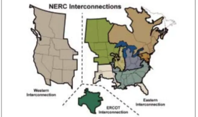
The National Transmission line system is currently divided into three regions; Western Interconnection, ERCOT Interconnection, and Eastern Interconnection as shown in Figure 1 below.

Figure 1: NERC Interconnections

Figure 1: North American Transmission Line Regions Source: National Transmission Grid Study, 2002

Currently, the US transmission grid uses 154,503 miles of high voltage AC

transmission lines and 3,307 miles of high voltage DC transmission lines ranging from 230 kV lines to 765 kV lines (National Transmission Grid Study, 2002). According to an article published in Technology Review, “These systems are far from orderly; each grid is composed of a tangle of transmission lines operated by a hodgepodge of owners, from sprawling federal power authorities to regulated utilities to market-savvy conglomerates. An equally variable set of state, regional and federal regulators governs aspects of this mosaic, deciding how much power can enter the grids and flow over each set of lines” (Fairley, 2001). Fairleyʼs

assertion of the disorderly nature of the US transmission grid was reconfirmed by Doug Smith of Van Ness Feldman, PC at the March 2009 AWEA Wind and Transmission Workshop that I attended this year for my thesis.

AWEA is the American Wind Energy Association which hosts many

workshops for wind developers and academics alike as well as hosting a website that is full of commercial and residential scale wind related information that is well respected in the wind industry. AWEA is also responsible for the AWEA

WINDPOWER Conference and Exhibition, which is “The worldʼs largest and most anticipated annual event for wind energy” (AWEA.org).

AWEA is an excellent resource to use when a person first considers getting into the wind industry. When that person decides to make the transition from merely being interested in the wind industry to wanting to develop a wind farm, some more detailed background information is necessary.

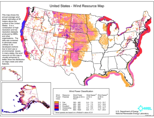
In order to develop a profitable wind farm, there are many factors that must be addressed. First, a location with a profitable wind speed needs to be identified. Wind speed is highly variable across the United States, as illustrated by Figure 2 below.

Figure 2: US Wind Speed Map

Figure 2: Illustration of wind speeds and its high variability across the United States. (windpoweringamerica.gov)

Wind speed is also highly variable throughout the day (AWEA.org). Capacity factor is the next variable that needs to be considered. Capacity factor is defined as “the actual amount of power produced over the power that would have been produced if the turbine operated at itʼs maximum output 100% of the time,” which is a function of the variable wind speeds throughout the day (AWEA.org). Next, the wind rose needs to be considered because along with local terrain, it is critical for determining turbine placement. A wind rose is an illustration of the distribution of wind speeds relative to the frequency of the direction of the wind

(windpower.org). After taking into consideration the wind speed, capacity factor, terrain, and wind rose of a location, another factor involved in preliminarily determining if a wind farm could potentially be developed in a location is the proximity to a transmission line and its open capacity to take on the energy generated by the potential wind farm. As previously discussed, the transmission line system in the United States does not have a central form of organization, so being close to a transmission line and having open capacity available on that line can make or break the development of a wind farm. Finally, land has to be

available either for sale or lease at economically feasible rates on which to develop the wind farm. Again, this is a critical factor.

The model developed for this thesis takes into account the economics of land value, the proximity of transmission lines, as well as capacity factor to create a dynamic model that can be used to preliminarily identify potential sites for wind development. Once a site is preliminarily identified through the use of this model, many other factors come into play such as availability on transmission lines, the willingness of locals to lease or sell their land, etc.

METHODS

ASSUMPTIONS:

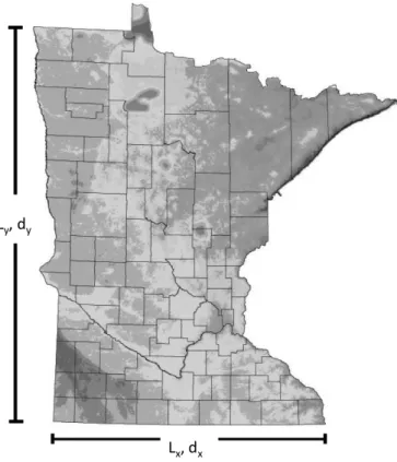
The state of Minnesota was chosen for this project because it has the most up to date and largest amount of publicly available data for wind farm development; specifically, capacity factor maps, wind speed maps, land value maps and wind resource maps. In the wind industry, it is common for a wind developer to pay a third party company that has expertise in wind analysis and also has access to meteorological tower data to compile maps for capacity factor, wind speed, and wind resource. The amount and thoroughness of free, publically available data made Minnesota an ideal candidate on which to run and test the model created for this thesis.

Several assumptions were used during the development of this model. First, maps of Minnesota accounting for land value, wind capacity factor, and transmission line locations were scaled to be the exact same size using Adobe Photoshop. Thus, each pixel on these maps is equivalent to 50 acres of land. To accomplish this, the bottom portion of the state of Minnesota was measured to be 263 miles using Google Earth Pro. The resolution of the image was set at 150 pixels per inch. The bottom portion of Minnesota was then measured in inches as 6.18 inches or a total of 928 pixels. A vertical portion of Minnesota was measured to ensure that the pixels of the image were indeed square and not rectangles. The vertical component measured 380 miles on Google Earth Pro and 9 inches

in Adobe Photoshop. Using the following conversion factors, it was calculated that 1 pixel was equal to 50 acres, see Figure 3 and Figure 4 below.

Figure 3: Illustration of Ly, dy, Lx, dx

Figure 4: Conversion Factors Used To Determine Pixel Dimensions

Figure 4: Explanation of the conversion factors used to determine acres per pixel as well as pixel dimensions

Next, the conservative estimate of two turbines per 50-acre plot of land was used to account for turbine density. In the wind industry, turbine density (i.e. how densely turbines are placed together) varies due to the topography and local vegetation, the consistency in the results of the wind rose, and also due to the agreement that the wind developer has with the landowner. For example, if the wind developer has the opportunity to buy the land under development, he or she would ideally like to optimize the turbine density in regard to the predominant wind direction, the topography, the capacity factor, the turbine blade length, and local zoning ordinances in regard to the edge of the property. Another common scenario in the wind industry occurs if the developer leases land from other landowners because it is not economically feasible to buy the land (i.e. it is too valuable for agricultural purposes) or if the landowner refuses to sell for

much land as possible from as many landowners as possible in the viable wind area. This will mean that the developer will “spread out” the turbines equally on the various landownersʼ properties in such a way that all landowners benefit from the revenue that will be generated due to wind royalties. It is uncommon to be able to lease land from a landowner without guaranteeing them a portion of the profits from the wind turbines as well as financially compensating the landowner for the land that is physically occupied by the turbines.

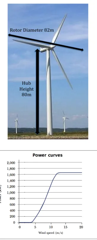
The turbine chosen for this analysis tool is the Vestas 1.65 MW turbine whose power curve, hub height and rotor diameter are shown below in Figure 5. This turbine was chosen because the map for capacity factor for the state of

Figure 5: Vestas 1.65 MW Turbine Specifications

Next, it was assumed that the electricity generated by the turbines would be sold at a rate of 5.82 cents per kilowatt-hour (americaspower.org) plus 1.5 cents per kilowatt-hour production tax credit (DSIRE). These numbers are arbitrary but are a reasonable estimate that can be easily manipulated in the model to suit the userʼs needs. The price of 5.82 cents was used based on the average retail selling price of electricity in the state of Minnesota that is 6.98 cents per kilowatt-hour marked up by 20% (a rough estimate). The rate for the production tax credit was used based on the Minnesota renewable energy production incentive

(DSIRE). At the moment there is no legislation mandating renewable energy credits (RECs) and the market is subject to high levels of volatility, and thus this potential source of profit was not included in this model at this time.

For the sake of explaining the model developed for this thesis, it was assumed that all financing is completely by loan that will be paid off over 20 years. However, this is highly variable in the industry and can be adjusted to suit the userʼs needs.

The numbers used to account for the cost of the turbines in relation to the turnkey costs as well as the operation and maintenance costs are industry averages (Burton et al, 2001). Also, since the terms of leases are highly variable in the industry, the model as it is explained in this paper used purchased land based on the value of the land per acre according to the State of Minnesota (state.mn.us). Again, the user can adjust this variable. Land tax is also accounted for in this model and is currently set to 2%, but can be adjusted to fit user needs.

This is not the actual percentage used in Minnesota. A developer would have to inquire at the local land office in order to get an accurate value for property tax.

Finally, in order to determine the cost of constructing transmission lines from a potential wind farm to an existing line, we assumed a cost of construction of $1 million per mile for the transmission line (Landauer and DeShazo, 2006). This number is arbitrary and user defined, but is based on current industry averages. In order to determine how much power can be carried on a

transmission line costing $1 million per mile, it was assumed that a transmission line costing $9 million per mile can carry 5 GW of power, therefore, a $1 million dollar per mile transmission line can carry 555 MW of power based on

information given at the AWEA transmission line conference by American

Superconductor Corporation. Since we are using a 1.65 MW wind turbine for this model, the transmission line that would be constructed according to this model (which is, again, arbitrary and user defined) would be able to handle a wind farm consisting of 336 turbines. In order to determine the cost per pixel, and

functioning under the assumption of 2 turbines per pixel, an appropriate distribution of the cost of the transmission line is allocated to each potential turbine (see Figure 12 for calculation).

PROCEDURE:

Each pixel on the capacity factor map, the land value map, and the

modeled as a potential wind development site and can have their own specific values for each variable. A spreadsheet was developed that combined the specifications of the turbine, the cost of purchasing a turbine, the cost of installing, maintaining, and operating the wind turbines, as well as the specific land value, capacity factor, and proximity to transmission lines for each pixel.

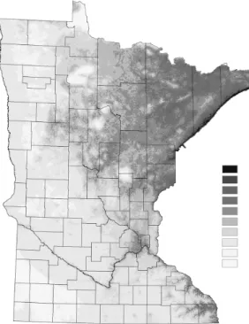
The capacity factor map and land value map that was publically available originally used color. The transmission line map, which was purchased from Platts, also originally came in color (platts.com). These maps are a combination of three layers of color; specifically red, green and blue. These maps were converted into grey scale black and white maps. This conversion simplified calculations that would be done later in Matlab. An example of an original map downloaded from the State of Minnesota Commerce website and its following Adobe Photoshop modifications is shown below in Figure 6 and Figure 7.

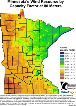
Figure 6: Original Capacity Factor Map in Color

Figure 6: A capacity factor map downloaded from the State of Minnesota Commerce website before modification (state.mn.us)

Minnesota's Wind Resource by Capacity Factor at 80 Meters

Turbine Capacity Factor 15.8% - 18.7% 18.7% - 21.6% 21.6% - 24.4% 24.4% - 27.3% 27.3% - 30.2% 30.2% - 33.1% 33.1% - 36.0% 36.0% - 38.8% 38.8% - 41.7% 41.7% - 44.6%

This map has been prepared under contract by WindLogics for the Department of Commerce using the best available weather data sources and the latest physics-based weather modeling technology and statistical techniques. The data that were used to develop the map have been statistically adjusted to accurately represent long-term (40 year) wind speeds over the state. Capacity factors are based on a 1.65 MW turbine, and production has been discounted 15% to represent real world conditions. Data has been averaged over a cell area 500 meters square, and within any one cell there could be features that increase or decrease the values shown on this map. This map shows the general variation of Minnesota’s wind resource and should not be used to determine the performance of specific projects. January 2006

Figure 7: Capacity Factor Map in Adobe Photoshop

Figure 7: The above figure is the same map as seen in Figure 6, but it has been properly modified in Adobe Photoshop and is ready to be imported into MatLab for further analysis

(state.mn.us)

Matlab recognizes the single color gradient used in the converted maps as matrices with each position containing a value from 0 to 256. The values ranging from 0 to 256 were converted to represent the specific information included in each map. For example, the darkest shade of black represented the lowest capacity factor on the now converted capacity factor map, see Figure 7 above. Once the maps were converted and appropriately scaled, appropriate code in Matlab was created to reflect the calculations done in the spreadsheet. In Matlab,

the calculations accounted for each pixel on the state map, thus creating a cost calculator in matrix form. Users who wish to use this model must input static information that will be applied to every pixel uniformly. For example, the cost of a turbine is going to remain constant regardless of where it is installed. The capacity factor, the proximity to transmission lines, and the land value, however, were dynamic across the state and gave each pixel a unique value. Below in Figure 8 is an example of MatLab code for importing the capacity factor map and scaling it appropriately.

Figure 8: MatLab Script for Capacity Factor Map

Figure 8: The above script allows MatLab to import the map seen in Figure 7 and appropriately convert all the pixels in Figure 7 into data points to form a matrix that can later be

used to create a cost analysis model for the state of Minnesota.

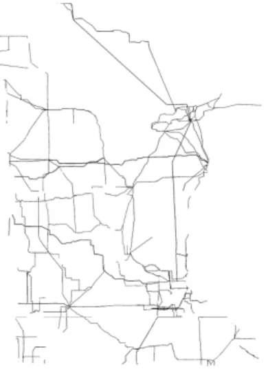
The transmission line map was not publicly available information and needed to be purchased. This map was also in color when it was downloaded from Platts. Using Adobe Photoshop, all colors were removed from the map and only

the transmission lines were left on the map as black lines. Superfluous

information, such as county lines, power producing territories, etc was removed from the map. Projected transmission lines were also removed from the map because according to an AWEA (American Wind Energy Association) conference on transmission lines that I attended for my thesis, it is well understood that the transmission grid needs substantial upgrades but that no one knows who is responsible for a nationwide design of a transmission grid that will be able to carry energy generated in the Midwest plains and the deserts of the Southwest to areas of high power demand, like the East Coast. Thus, the location of the

projected transmission lines included in the Platt map is arbitrary in nature. If at some point in the future the government does announce a coordinated national initiative to upgrade the US transmission line system, this can easily be

incorporated into the model in order to see which areas become feasible when new transmission lines are built.

Importing the transmission line map proved to be challenging. After removing unnecessary information from the Platt transmission line map, it was ready to be imported into MatLab with a white background with only solid black color to represent the transmission lines as illustrated by Figure 9 below.

Figure 9: Transmission Line Map for MatLab Analysis

Figure 9: Transmission line map as it was imported into MatLab showing only existing transmission lines in black color (platts.com)

In order to calculate transmission line proximity, first a logical test was performed over the whole map where if a pixel was a transmission line, it was given a value of 1, and if a pixel was not a transmission line, it was given a value of 0. Then, MatLab identified the coordinates of all the pixels that represented transmission lines. Finally, a repetitive task was performed to determine the distance of every pixel on the map from every pixel that represented a

transmission line using the Pythagorean theorem. Next, MatLab had to determine the minimum distance for every pixel on the map to the nearest transmission line in order to identify the most proximal transmission line for every pixel on the map. MatLab required approximately fifteen hours to identify the most proximal

MatLab script for this process, a much smaller portion of the transmission line map was used in order to save time while perfecting the script. The test map is illustrated below in Figure 10.

Figure 10: Test Transmission Line Map

Figure 10: The test transmission line map with dimensions of 104 by 109 pixels that was used to perfect the proximal transmission line MatLab script.

Next, a spreadsheet was used to develop a cost analysis model that accounted for the following variables: capacity factor (a dynamic variable which was determined by the relevant map), land value per acre (a dynamic variable which was determined by the relevant map), transmission line proximity (a dynamic variable which was determined by the relevant map), as well as user determined variables as follows: the rated power of the turbine, the number of turbines per pixel, the selling price of electricity per kilowatt hour, the interest rate at which a loan would be issued, the property tax per year, the cost of the turbine, the cost of the transmission line per mile to construct, the average power output of the turbine per pixel, the annual production of electricity in kilowatt hours per pixel, the income per year per pixel, the operation and maintenance costs per pixel per year, the number of payments for the debt over 20 years, and the debt payment per year. This cost analysis model accounts for the operation and expected profits or losses of an arbitrarily sized wind farm that has two turbines

per 50 acres (per pixel) from a year to year basis, but can be easily modified to suit a userʼs needs.

The spreadsheet was then incorporated into MatLab along with the previously discussed maps to develop the dynamic model, which shows the areas of

Minnesota that are feasible for wind development. The annual income was

calculated by multiplying the turbineʼs rated power times the capacity factor times the number of turbines per pixel times 365 days per year times 24 hours per day times the selling price of electricity per kilowatt hour as illustrated by Figure 11 below.

Figure 11: Calculation of Annual Income

Figure 11: The annual income of a one pixel wind farm. All variables (n= number of turbines, P= rated power of turbine, cf= capacity factor, average power per year per pixel, annual energy output in kilowatt hours, selling price of electricity in dollars per kilowatt hour, annual income per pixel) are user defined in the previously discussed spread sheet, except for capacity factor, which

The annual expenses were then taken into account. The annual expenses are operation and maintenance, the annual debt payment, and property taxes as illustrated by Figure 12 below.

Figure 12: Calculation of Annual Expenses

Figure 12: The annual expenses of a one-pixel wind farm. All variables (O&M= operation and maintenance costs, Cost= total cost for building turbines and transmission lines per pixel, r= rate of interest on the loan, y= number of payments over 20 years, annual debt payment, land value

per acre, annual property tax) are user defined except for d, which is a function of the transmission line proximity map, and land value per acre, which is a function of the land value

map.

Finally, overall profit per pixel was determined as income minus expenses, which include operations and maintenance, annual debt payment, and annual property tax as illustrated by Figure 13 below.

Figure 13: Calculation of Annual Profit Per Pixel

Figure 13: The annual profit of a one-pixel wind farm. Profit is a function of income minus operations and maintenance costs, annual debt payments, and minus annual property tax

RESULTS

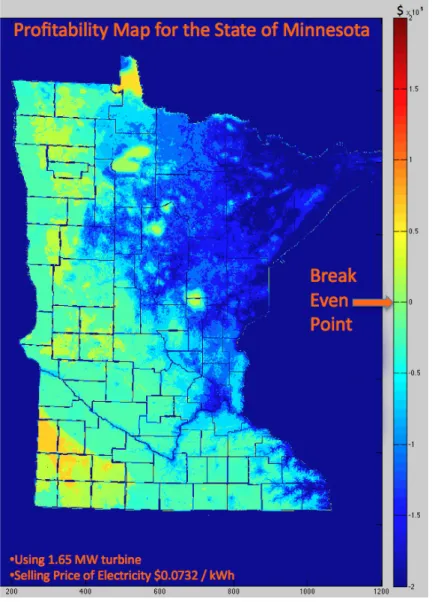
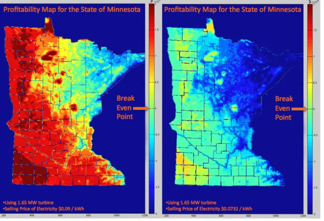
The map that was generated from this cost analysis model based on the previously mentioned assumptions can be seen in Figure 14 below. The color bar shows whether an area is likely to be profitable or not based on the previously discussed parameters. The values represent annual profit in dollars.

Figure 14: Result Map

Figure 14: Map showing profitability of areas by color with the selling price of 7.32 cents per kilowatt-hour as mentioned before.

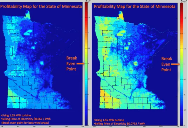
If all parameters remain static but the selling price of electricity is adjusted to 9 cents per kilowatt-hour because of new subsidies such as renewable energy credits then the following resulting map is generated shown in Figure 15 below. Other scenarios are also presented below in Figures 16 (break even point for areas with best wind), and 17 (price of turbines drops by 20%).

Figure 15: Result map with selling price of 9 cents per kilowatt-hour (left)

Figure 15: Map showing profitability of areas by color assuming selling price of electricity is 9 cents per kilowatt-hour (left) compared to result map with the assumed price of 7.32 cents per

Figure 16: Result map with selling price of 6.7 cents per kilowatt-hour, the break-even point for areas with best wind (left)

Figure 16: Map showing profitability of areas by color assuming selling price is 6.7 cents per kilowatt-hour (left) compared to current assumed selling price as in Figure 14 (right). At this selling price, only wind farms in the areas with the best wind would break even (green color). Government officials or utility companies could use this tool to think about their long-term goals as

organizations. For example, if the state of Minnesota would like 40% of their electricity to be generated by wind, then they could adjust this analysis tool to generate appropriate forecasts for

Figure 17: Result map with price of turbines dropping by 20% (left)

Figure 17: Map showing profitability of areas by color assuming the cost of turbines drops by 20% (left) compared to current assumed selling price as in Figure 14 (right). This could be a scenario

that develops in the future because of technological advances as well as material science advances used in manufacturing wind turbines that could drive the costs of producing the turbines

CONCLUSIONS

Overall, there was a high correlation between where the model predicted that wind farms should be developed and where wind farms actually exist today in Minnesota. For example, the model identified the southwest corner of

Minnesota as an ideal location for wind farm development. This also happens to be one of the most densely populated areas concerning wind farm development in the state as illustrated by Figure 14 in “RESULTS” and Figure 18 below.

Figure 18: Current location of wind farms in Minnesota today

Figure 18: Map showing current wind turbine locations across the State of Minnesota (state.mn.us) compared to Figure 14.

However, the model also identified a section of the northwest corner of Minnesota as a potential site for wind farm development. It should be noted that to this day, such development has not taken place. There are many reasons why wind farm development may not be under way in this area of Minnesota. For example, landowners may be highly resistant to wind farm development and thus are unwilling to sell or lease their land to wind farm developers. Also, open

transmission capacity may not be available on the transmission lines running through the area at this time or the utilities that control the lines may not be

granting permission for wind integration into their lines at this time. These are just two possible examples out of many possibilities as to why the northwest corner of Minnesota, which has very good wind capacity factors, cheap land, and also transmission lines present, is not currently under development. At this time, the model is not able to account for certain factors, such as local resistance to wind farm development or open availability on transmission lines.

The map of current wind farms in the state of Minnesota (Appendix A) also shows a region in the southeast corner of the state where there are several wind farms operating. Based on the initial values assumed for all the variables in the analysis tool discussed, this area is not presented as an area that is attractive for wind farm development (see Figure 18 above). One reason for this unexpected development might be that the wind farms already in existence in that area provide electricity for utility companies in other states that offer a higher selling price than the estimated 7.32 cents per kilowatt-hour suggested in this analysis

tool. Another reason for this discrepancy might be the fact that the wind farms in that area are using a wind turbine that has a higher capacity factor for the same wind speed, thus these turbines are able to generate more electricity than the 1.65 MW turbine used in this analysis tool, and are thus generating more income. Also, it is possible that the selling price of electricity per kilowatt-hour that is assumed for the state of Minnesota is an underestimate.

The analysis tool also assumes that the cost of constructing transmission lines is allocated to 336 turbines. This means that a developer using this tool would be looking at the capital costs, expenses, and revenue per pixel based on the fact that he or she would be developing a wind farm in the order of 336 turbines or 555 MW. If, however, a developer would be using this tool with the intentions of building a wind farm with only 34 turbines, then he or she would have to allocate the cost of constructing transmission lines to 34 turbines. Figure 19 below shows a comparison of how the cost of transmission lines effects the viability of a project depending on the number of turbines to be constructed. As can be seen in Figure 19, the larger the wind farm one considers, the less of a factor constructing transmission lines becomes. For example, developer A is considering building a 50 MW wind farm (about 30 turbines) that requires construction of 20 miles of transmission lines. Based on the $1 million per mile estimate, the developer will need to invest $20 million in transmission lines and $105 million in turbines for a total of $125 million. The cost of constructing the 20-mile transmission line is roughly 16% of the total capital cost for the project.

Developer B is considering building a 500 MW wind farm (about 300 turbines) that also require construction of 20 miles of transmission lines. His total capital cost will be $20 million for the transmission line and $1.05 billion for the turbines. The cost of constructing the 20-mile transmission line is roughly 2% of the total capital cost for developer B.

Figure 19: Comparison of effect of transmission line cost for a large and small wind farm developer

Figure 19: The map on the left is one showing profit or loss for a wind farm developer who is considering building a wind farm in the order of 336 turbines. The map on the right is one showing

the corresponding profit or loss for a wind farm developer who is considering building a wind farm on the order of 34 turbines, 10% the size of the wind farm on the left map.

This model could be further developed in the future to account for more complex variables such as availability of power on transmission lines, cost of transmission line per mile based on a specific voltage line, resistance of landowners to selling their land to wind farm developers, etc. Currently, this model can be manipulated for the following variables: Static and user defined

variables per pixel: price of electricity, price of turbines, construction of

farm, debt financing, type of turbine, property tax; Dynamic and map defined

variables per pixel: capacity factor, transmission line proximity, and land value.

DISCUSSION

The purpose of this thesis was to create a model that would immediately account for simple variables such as capacity factor and price of electricity, but that could easily be expanded in the future to account for a change in variables or more variables, whether static and/or dynamic, such as if the price of electricity changes rapidly with time, or a new government subsidy for electricity produced from wind was created nationwide, or if all federal and state controlled lands are opened for wind development at extremely favorable lease rates (a dynamic, map defined variable).

For example, assume that the government mandates a $0.03 per kilowatt-hour CO2 tax credit on top of the current producerʼs tax credit (currently at 1.5

cents per kilowatt-hour) and the current selling price of electricity (arbitrarily chosen as 5.82 cents per kilowatt hour). This new static variable makes the total price of electricity per kilowatt-hour that the wind developer could count as income increase from 7.32 cents to 10.32 cents per kilowatt-hour. The model would then consider areas with poorer capacity factors or more expensive land as being financially viable for wind farm development.

Being able to predict the effect of such a government mandate could give a wind developer an edge over the competition in determining what land to buy or lease for long-term development. If this model was adapted to account for all 50 states, it could be used as a starting point to determine what price government subsidies need to be set at in order for more than 20% of Americaʼs electrical energy to come from wind. Currently, 20% of Americaʼs electricity could be generated from wind (AWEA.org). However, if the US wanted 50% of its energy to come from wind, government subsidies would likely be necessary to make formerly unprofitable areas (due to high land price, or poorer capacity factor ratings) to become profitable for wind farm development, “According to the U.S. Department of Energy, the world's winds could theoretically supply the equivalent of 5,800 quadrillion BTUs (quads) of energy each year—more than 15 times current world energy demand” (AWEA.org).

Also, with advances in material sciences, a turbine with a much larger tower and rotor diameter than is currently used in the industry, could be

developed and become cost effective for production. Advances in turbine design such as this could allow locations with previously unprofitable wind, such as low capacity factors and high land values, to become profitable for wind farm

development. This model can currently take into account such advancements in wind turbine development so long as the cost of the turbine and its capacity factor for electrical production is known.

Future work on this model could focus on launching it in a popular and publicly available form that can be updated in real time, such as an application for Google Earth. As use of and capabilities of web based applications expand, the launching of this model on Google Earth could become possible. Current

limitations, such as 15 hours of MatLab calculations to determine proximity to transmission lines for the State of Minnesota alone, would be exorbitant if one was trying to calculate on a national scale at this time. This model would currently be ideal for wind farm developers that are considering specific areas as potential sites for wind farm development that are on the scale of US states or smaller.

APPENDICES

COTTONWOOD BLUE EARTH PENNINGTON OTTER TAIL YELLOW MEDICINE W A S H IN G T O N M IL L E L A C S

Wind Turbines in Minnesota

Legend

Not Permitted by PUC (291) Permitted by PUC (1040)

Interstate Highways US Highways State Highways Counties

Prepared for the Minnesota Department of Commerce Energy Facility Permitting by the Department of Administration's Land Management Information Center, Jan 2009.

Map document: statewide_2008photo.mxd 0 15 30 60

Miles

* Number of turbines in parenthesis ( ) Permitted by PUC refers to those permitted by the Minnesota Public Utilities Commission.

Includes known wind turbines locations. Sites were determined by review of sites that appear in the FAA Obstruction Database as of December, 2008 and veritfied against the Minnesota Air Photos 2008, collected as part of the U.S. Department of Agriculture's National Agriculture Imagery Program (NAIP).

Bibliography

American Wind Energy Association. (2009). AWEA. Retrieved April 18, 2009, from http://www.awea.org/ 

Burton, T., Sharpe, D., Jenkins, N., & Bossanyi, E. (2001). Wind Energy

Handbook. Chichester: John Wiley and Sons.

Fairley, P. (2001, July). A Smarter Power Grid. Technology Review. Retrieved April 10, 2009, from http://www.technologyreview.com/Energy/12474/page2/ Landauer, M., & DeShazo, G. (2006, May 16). Canada–Northwest–California

Transmission Options Study [Northwest Power Pool Northwest Transmission

Assessment Committee Canada-NW-California Study

Group ]. Retrieved May 7, 2009, from http://www.nwpp.org/ntac/pdf/ CNC%20Report%20-%20Final%2016%20May%202006.pdf

Minnesota. (2007). DSIRE [Incentives By State]. Retrieved May 7, 2009, from NC State University Web site: http://www.dsireusa.org/library/includes/

incentive2.cfm?Incentive_Code=MN06F&state=MN&CurrentPageID=1 &RE=1&E=1

Minnesota. (2009). America's Power [The Facts]. Retrieved May 7, 2009, from American Coalition For Clean Coal Electricity Web site:

http://www.americaspower.org/The-Facts/

National Transmission Grid Study. (May 2002). U.S. Department of Energy: U.S.

Department of Energy The Honorable Spencer Abraham Secretary of Energy.

Platts [Maps and Spatial Software]. (2009). Retrieved May 5, 2009, from

http://www.platts.com/Maps%20&%20Spatial%20Software/

United States- 50 m Wind Resource Map. (2009, March). Wind Powering

America [State and United States Wind Resource Map]. Retrieved April 14,

2009, from US Department of Energy: Energy Efficiency and Renewable Energy Web site: http://www.windpoweringamerica.gov/wind_maps.asp 

Wind Maps [2006 Wind Maps]. (2000). Retrieved April 24, 2009, from Minnesota

Department of Commerce Web site: http://www.state.mn.us/portal/mn/jsp/ content.do?contentid=536887066&contenttype=EDITORIAL&

The Wind Rose. (2003). Danish Wind Industry Association [www.windpower.org]. Retrieved April 1, 2009, from Danish Wind Industry Association Web site: http://www.windpower.org/en/tour/wres/rose.htm