HAL Id: hal-00317823
https://hal.archives-ouvertes.fr/hal-00317823
Submitted on 28 Jul 2005
HAL is a multi-disciplinary open access
archive for the deposit and dissemination of
sci-entific research documents, whether they are
pub-lished or not. The documents may come from
teaching and research institutions in France or
abroad, or from public or private research centers.
L’archive ouverte pluridisciplinaire HAL, est
destinée au dépôt et à la diffusion de documents
scientifiques de niveau recherche, publiés ou non,
émanant des établissements d’enseignement et de
recherche français ou étrangers, des laboratoires
publics ou privés.
A quantitative analysis of the diurnal evolution of
Ionospheric Alfvén resonator magnetic resonance
features and calculation of changing IAR parameters
S. R. Hebden, T. R. Robinson, D. M. Wright, T. Yeoman, T. Raita, T.
Bösinger
To cite this version:
S. R. Hebden, T. R. Robinson, D. M. Wright, T. Yeoman, T. Raita, et al.. A quantitative analysis of
the diurnal evolution of Ionospheric Alfvén resonator magnetic resonance features and calculation of
changing IAR parameters. Annales Geophysicae, European Geosciences Union, 2005, 23 (5),
pp.1711-1721. �hal-00317823�
Annales Geophysicae, 23, 1711–1721, 2005 SRef-ID: 1432-0576/ag/2005-23-1711 © European Geosciences Union 2005
Annales
Geophysicae
A quantitative analysis of the diurnal evolution of Ionospheric
Alfv´en resonator magnetic resonance features and calculation of
changing IAR parameters
S. R. Hebden1, T. R. Robinson1, D. M. Wright1, T. Yeoman1, T. Raita2, and T. B¨osinger3
1Dept. of Phys. and Astronomy, Univ. of Leicester, Univ. Road, Leicester, LE1 7RH, UK 2Sodankyl¨a Geophysical Observatory, T¨ahtel¨antie 62, 99600 Sodankyl¨a, Finland
3Dept. of Phys. Sciences, Div. of Physics, Sect. of Space Phys. Res., P. O. Box 3000, 90014 University of Oulu, Finland
Received: 29 September 2004 – Revised: 6 April 2005 – Accepted: 8 April 2005 – Published: 28 July 2005
Abstract. Resonance features of the Ionospheric Alfv´en
Resonator (IAR) can be observed in pulsation magnetometer data from Sodankyl¨a, Finland using dynamic spectra visual-izations. IAR resonance features were identified on 13 of 30 days in October 1998, with resonance structures lasting for 3 or more hours over 10 intervals. The diurnal evolution of the harmonic features was quantified for these 10 intervals us-ing a manual cursor-clickus-ing technique. The resonance fea-tures displayed strong linear relationships between harmonic frequency and harmonic number for all of the time intervals studied, enabling a homogeneous cavity model for the IAR to be adopted to interpret the data. This enabled the diurnal variation of the effective size of the IAR to be obtained for each of the 10 time intervals. The average effective size was found to be 530 km, and to have an average variation of 32% over each time interval: small compared to the average varia-tion in Alfv´en velocity of 61%. Thus the diurnal variavaria-tion of the harmonics is chiefly caused by the changing plasma den-sity within the IAR due to changing insolation. This study confirms Odzimek (2004) that the dominating factor affect-ing the IAR eigenfrequencies is the variation in the Alfv´en velocity at the F-layer ion-density peak, with the changing IAR size affecting the IAR eigenfrequencies to a smaller ex-tent. Another IAR parameter was derived from the analy-sis of the IAR resonance features associated with the phase matching structure of the standing waves in the IAR. This parameter varied over the time intervals studied by 20% on average, possibly due to changing ionospheric conductivity.
Keywords. Ionosphere (Auroral ionosphere; Wave
propaga-tion) – Radio science (Electromagnetic noise and interfer-ence)
Correspondence to: S. R. Hebden
(sophiehebden@yahoo.com)
1 Introduction
The Ionospheric Alfv´en Resonator (IAR) is the term given to the vertical structure associated with the decay in plasma density going from the ionosphere to the magnetosphere, whose existence was first predicted by Polyakov, (1976). Alfv´en waves propagating along the geomagnetic field lines are partially reflected from regions of large Alfv´en velocity gradients. The lower boundary region occurs in the iono-spheric F-layer. The upper boundary of the IAR corresponds to the region where the Alfv´en waves of interest undergo par-tial reflection at the large Alfv´en velocity gradient caused by the rapid decrease in plasma density above the F-layer density peak, whilst the geomagnetic field strength decreases with altitude more slowly.
IAR resonance features at high latitudes are observable in the electromagnetic spectra between 0.2 and 5 Hz (The fre-quency range of Pc1 waves) (Belyaev et al., 1999). These eigenfrequencies of the IAR were first observed in 1985 by Belyaev et al. (1987) in the form of multiple horizontally banded spectral resonance structures (SRS) in frequency-time plots of mid-latitude magnetic background noise be-tween 0.1 Hz and 10 Hz derived from pulsation magnetome-ter data. They were observed at high latitudes (L∼6, where L-shell value relates to latitude as L=cos−2λ
E)by Belyaev et al. (1999).
IAR resonance features are manifested in the form of mul-tiple maxima and minima in the magnetic field power spec-trum which are quite stable, often lasting for several hours until fading out or being masked by more intense wave ac-tivity. The modulation depth of the power spectrum can be up to 50%, and the frequency interval 1f between the peaks is generally in the range 0.5–3 Hz at mid-latitudes (Belyaev et al., 2000). They are regularly observed at low and mid latitudes in high time resolution magnetometer data, espe-cially at night-time. Belyaev et al. (1990) observed diur-nal variations of resonance peak characteristics in one of the
1712 S. R. Hebden et al.: A quantitative analysis of diurnal evolution two orthogonal components of the tangential magnetic field
at the Earth’s surface at the mid latitude station of Nizhny Novgorod (L∼2.6). The diurnal variation in frequency and spacing was proportional to 1/f0F2, where f0F2 is the crit-ical frequency of the F2-layer in the ionosphere. The reso-nance peaks increased in modulation depth, frequency and spacing towards the maximum at midnight and decreased to-wards dawn, with resonance features rarely observed during the day. These authors attributed the characteristics of the spectral resonance features to the changing parameters of the IAR.
Hickey et al. (1996) extended the observation at Nizhny Novgorod by reporting detection of banded magnetic spectra from an L∼1.5 station in California. The first evidence for the IAR at high latitudes (Belyaev et al., 1999) was in the form of resonance features observed on 4 out of 12 nights of data collection using the sensitive magnetometer experi-ment at Kilpisj¨arvi, Finland in November 1993. These au-thors qualitatively compared the frequency evolution of the resonance features with the change in ionospheric electron density from EISCAT (Rishbeth and Williams, 1985) inco-herent scatter radar data. Resonance features were reported by Demekhov et al. (2000) to be “a regular feature” at the high latitude magnetometer station at Sodankyl¨a, Finland (L∼5.1). These authors presented 4 days of observations from the stations at Nizhny Novgorod and Sodankyl¨a, Fin-land, and used a model of the IAR (published in Izvestiya vuzov-Radiofizika by Belyaev et al. in 1989) to make quanti-tative comparisons of the predicted spectra with the magnetic features. They found that the diurnal variation of the spectral resonance features could be well explained by the variation in the local ionospheric parameters.
More recently Yahnin et al. (2003) used continuous ob-servations from 1995–1999 at the Sodankyl¨a magnetometer station to define the morphology of the IAR resonance fea-tures at high latitudes. These authors found the occurrence rate (P ) of resonance features to be higher in the nighttime than the daytime, and higher in winter than in summer. They made a statistical study on the frequency spacing of the IAR eigenfrequencies (1f ) and of P , and showed that their diur-nal, seasonal and long-term behaviour agreed well with IAR theory predictions based on numerical calculations of the re-flection coefficient at the top-side ionosphere. These authors concluded that observations of SRS could be used for esti-mation of upper ionosphere parameters and for improving the existing ionosphere models.
In this paper, the evolution of the resonant frequencies with local time is quantified for days when they were clearly visible. Spectra from a whole month of pulsation magne-tometer data from Sodankyl¨a, Finland are considered. To interpret the data, a simple 1-D vertical model was adopted (Trakhtengerts et al., 2000) in which the IAR consists of 3 layers of constant density. The middle layer represents the standing wave cavity which is bounded below by a conduc-tion layer and above by a low density layer leading to the wave trapping and resonance features of the IAR. Data from a co-located ionosonde were combined with the IAR
reso-nance feature analysis results to calculate IAR model param-eters which correspond to the effective IAR cavity size and the phase matching structure of the standing wave in the IAR cavity.
This study confirms the earlier results that the diurnal lution of the IAR resonance features is caused by the evo-lution of the local IAR parameters via detailed day-by-day spectral analysis. It also illustrates the need for experimen-tal investigation of the reflection of Alfv´en waves at the lower boundary region of the ionosphere and how this re-lates to the ionospheric conductivity. Although this study is inconclusive on this point due to a lack of incoherent scat-ter radar data when IAR resonance features were observed in October 1998, it shows that linear relationships between the frequency f and harmonic number N of resonance fea-tures enable the reflection characteristics of Alfv´en waves at the lower boundary to be investigated using the simple IAR model.
2 Experimental data and processing method
October 1998 was chosen for this study of the structure of the IAR because during this month the University of Leicester ran some modulated ionospheric heating experiments at the Tromsø HF heating facility (Stubbe et al., 1982) to coincide with overhead passes of the FAST satellite (Carlson et al., 1998). In one of the heating experiments, narrow-band elec-tric and particle flux signatures were observed by the satellite for about 4 s (Robinson et al., 2000, Kolesnikova et al., 2002, Cash et al., 2002, Wright et al., 2003). This occurred when the satellite traversed magnetic flux tubes that map down to the heated ionospheric patch. The data were best explained by the presence of the IAR with an upper boundary ∼850 km above the satellite altitude (Cash et al., 2002). Thus any ad-ditional evidence for the existence of the IAR at similar lat-itudes in October 1998 makes the IAR interpretation of the FAST satellite data more convincing. By studying a month of data it is possible to ascertain how frequently IAR reso-nance features can be observed, and the common ionospheric conditions occurring during the observations. There are cur-rently several pulsation magnetometers located in northern Scandinavia (see Fig. 1), but only data from the Sodankyl¨a (SOD) pulsation magnetometer station (67.40◦N, 26.60◦E geographic coordinates) were available with high accuracy timing for October 1998.
Figure 2 provides an example of typical magnetic IAR res-onance features seen during the month of October 1998. It shows a 12-h colour dynamic power spectrum on 4th Octo-ber 1998 for the linear east-west (or D component) polariza-tion of differential magnetic field. Power spectral density is shown in colour scale normalized to a reference frequency of 3 Hz. This means that the maximum power occurring in the 3 Hz bin sets the maximum for the colour scale (maxi-mum=red). This is plotted as a function of hour of the day (x axis) and frequency (y axis). A lower threshold of 40% of the peak power was chosen because this produced the clearest
S. R. Hebden et al.: A quantitative analysis of diurnal evolution 1713
Figure 1. The Finnish pulsation magnetometer chain
Fig. 1. The Finnish pulsation magnetometer chain (courtesy of
SGO).
Figure 2. Uncalibrated D component pulsation magnetometer data for 04/10/98 from Sodankyla, Finland displayed as colour dynamic power spectra. Window and slip size are 100 seconds. Power Spectral density is normalised to peak power at 3 Hz.
a) 12:00 14:00 16:00 18:00 20:00 22:00 UT 0 1 2 3 4 5 6 7 f (Hz) 12:00 14:00 16:00 18:00 20:00 22:00 UT 0 1 2 3 4 5 6 7 f (Hz) 0.50 0.55 0.60 0.65 0.70 0.75 0.80 0.85 0.90 0.95
Fraction of Peak Power
Fig. 2. Pulsation magnetometer data for 04/10/98 from Sodankyl¨a,
Finland displayed as colour dynamic power spectral plot for the east west (D component) polarisation. The window and slip size are 100 s; power spectral density is normalised to peak power at 3 Hz and not calibrated.
resonance features, below the threshold a spectral component is omitted from the plot. The dynamic spectrum was pro-duced by applying a Fast Fourier Transform (FFT) to a slid-ing window of 100 s, and movslid-ing it along by increments of 100 s along the differential magnetic field time series. Thus the frequency resolution is 0.01 Hz and the time resolution is 100 s. At each time-slip along the data series, the DC com-ponent in the data within the FFT window is removed, then the window is convolved with a standard Hanning window (Lynn, 1984) to minimise the number of terms in the fre-quency response of the window. This is effectively a “raised cosine bell” function applied to 10% of the data points at each edge of the window.
The magnetic data used throughout this paper were not calibrated for the frequency response of the magnetometer because the sensitivity of the search coil sensors increases with frequency up to 3 Hz. This is an advantage because the weak IAR resonance peaks around 3 Hz are easier to observe,
0 1 2 3 4 5 f (Hz) 0 10 20 30 40 50 Po w er sp ec tra l d en si ty (p T 2)
Figure 3. Calibrated D component magnetic power spectral density for
1800-1840 UT on 04/10/98 for window and slip size 100 s. This is the average of 24 power spectra, smoothed with a boxcar of width 3.
Fig. 3. Power spectral density for 18:00–18:40 UT from pulsation
magnetometer at Sodankyl¨a, Finland on 4 October 1998 for window and slip size of 100 s. This is the average of 24 power spectra, smoothed with a boxcar of width 3.
whilst the magnetometer is less sensitive to the naturally high amplitude Pc1 waves at about 0.3 Hz.
With reference to Fig. 2, the resonance features appear at about 16:00 UT as 9–10 coloured horizontal bands roughly equally spaced in frequency, and slowly increasing in fre-quency and frefre-quency spacing (1f ) with time towards mid-night. The remaining linear north-south (H component) and circular polarization components (RH and LH components which are not shown) occur at the same frequencies as the east-west component displayed in Fig. 2, but are of slightly lower amplitude, not distinguishable as resonance features until 18:00 UT. The power spectral density in the D compo-nent is ∼10 pT2/ Hz from 0–3 Hz at 18:00 UT (see Fig. 3), but it varies in time differently for each polarization. How-ever, it is possible to use the persistence in time of the reso-nance features to detect their presence in the data. Pc1 waves can be seen at almost all times in Fig. 2 at frequencies below 0.5 Hz. However, true IAR resonance features (with more than one harmonic) are observable in the D component from about 16:00 UT until midnight. The modulation depth be-tween peaks and troughs is best determined from a single calibrated differential power spectrum, shown for the D com-ponent in Fig. 3 for 18:00–18:40 UT on 4th October 1998. This plot is the average of 24 individual spectra of 100 s of data, thus it has a time resolution of 40 min and frequency resolution of 0.01 Hz. Averaging over 24 spectra removes the ephemeral features in the data leaving the coherent res-onance features. It can be seen that the modulation depth between peaks and troughs is ∼5–10 pT2/Hz in the range 0– 3 Hz, or ∼50% of the peak power at this time.
Dynamic spectra were plotted for every day in October except 16th October 1998 when there were data gaps. Res-onance features of the IAR in the form of multiple har-monic bands that evolve in frequency with time were ob-served on 13 days. Considering the geomagnetic activity during October, resonance features were observed on 9 out of 10 days when the average daily Ap<5, and only 4 out of 20 days when Ap≥5. The 3rd October 1998 had the
max-1714 S. R. Hebden et al.: A quantitative analysis of diurnal evolution Sp ec tra l P ow er ( ar bi ta ry u ni ts ) f (Hz)
Figure 4. Stack plot of uncalibrated 20 minute-averaged power spectra for the
D component magnetic field on 04/10/98. The spectra are from 16.40-19 UT, going from blue-orange with time.
Fig. 4. Stack plot of 20 min-averaged power spectra for the east
west (D component) polarisation magnetic field on 4 October 1998 from pulsation magnetometer at Sodankyl¨a, Finland. The spectra are from 16:40–19:00 UT going from purple to orange with increas-ing time. 16 18 20 22 24 Time UT 0 1 2 3 4 5 Fr eq ue nc y (H z)
Figure 5. Spectral resonance features for 04/10/98 H component
polarization. The frequency variation over time for the first 8 harmonics was derived using method 1, using averaged spectra which represent 20 minutes of data. The error bars give the uncertainty in frequency of the resonance peaks.
Fig. 5. Spectral resonance features on 4 October 1998 for the north
south (H component) polarisation magnetic field from Sodankyl¨a, Finland. The frequency variation over time for the first 8 harmonics was derived using averaged spectra, which represent 20 min of data. The error bars give the uncertainty in frequency of the resonance peaks.
imum average daily Ap on which resonance features were observed. For this day the average Ap was 13.6, although the resonance features occurred during the afternoon when the Apindex dropped to 3 or 4. This corresponded with the end of ULF wave activity, and a flattening out of the spec-tra after midday. For the 7 days in October 1998 with dis-turbed magnetospheric conditions (Ap>20), IAR resonance features were never observed since there was intense, highly variable ULF wave activity flooding the spectra and masking the background noise in which the resonance features appear. Quantifying the diurnal frequency variation of the IAR resonance features is difficult because of the low modulation depth in the harmonic peaks at any instance in time. In at-tempts to find a quick and accurate technique to quantify the SRS features, two different manual methods were developed that exploit the coherence between consecutive spectra. An automated method was used to compare the change in 1f
with time and thus to validate the manual method used for the data analysis.
2.1 Method 1
The first method was based on the spectral resonance feature visualisation used by Belyaev et al. (1999). Each polarization was processed by taking an FFT of a 10-s window of data and moving the window along by 10 s, and then averaging over 120 spectra. This produced spectra like Fig. 3 with a time resolution of 20 min and a frequency resolution of 0.1 Hz, which were displayed as stack plots to show the diurnal evo-lution of the resonance features. Figure 4 is an example of a series of uncalibrated spectra for D component polarization on 4th October 1998 from 16:40–19:00 UT. The IAR reso-nance peaks are more easily identifiable in the context of a few hours of stack plots because they are extremely coherent in time. The peak frequencies, their amplitudes and uncer-tainties were determined for each 20 min spectrum, at each polarization using the on-screen interactive cursor clicking technique. An average of the four polarizations was taken to give the most accurate diurnal evolution of the spectral res-onance features. An example of the variation in frequency with time for 8 harmonics in the afternoon of 4th October 1998 for the H component polarization is shown in Fig. 5, with the error bars given by the uncertainty in judging the peak frequencies. The frequency spacing between peaks in-creased by 0.21 Hz from 17:00–22:00 UT.
2.2 Method 2
To determine the variation in the frequency spacing between harmonics (1f ) with time, an automated method was used that relies on the regular spacing of IAR harmonics in the magnetic power spectra. This method treats the stack plots of spectra used in method 1 as mini time series of data con-taining a fixed period wave (since harmonics of the IAR are equally spaced in frequency). FFTs of these spectra were performed to obtain “pseudo spectra”. A peak in a pseudo spectrum indicates that there are multiple harmonics present in the real spectrum, and the inverse of the “pseudo fre-quency” of the peak gives 1f . Figure 6 columns 2 and 4 illustrate the change of the pseudo frequency peak with time. Time increases by 20 min per panel going from top to bot-tom. The main peak decreases in pseudo frequency with time, thus the pseudo wavelength increases. Therefore the spacing of the peaks (1f ) in the real spectra increases by 0.20 Hz; this matches the value obtained using method 1 to within 0.01 Hz. Thus this method confirms the result from method 1 for 17:00–22:00 UT on 4th October 1998.
2.3 Method 3
The third technique allows the diurnal evolution of the har-monic frequencies to be quantified (only frequency spacing is quantified using the automated method) more quickly than method 1 and with greater accuracy as a consequence of the 20 min time resolution of each spectral plot for method 1.
S. R. Hebden et al.: A quantitative analysis of diurnal evolution 1715 Method 3 used dynamic spectra for 12-h sections of data;
visualisations like that displayed in Fig. 2. These were plot-ted on the computer screen for each of the four polarization components at maximum pixel resolution so that the reso-nance features could be identified interactively with the cur-sor. Where a harmonic peak was visible above the back-ground level, the variation in frequency with time was de-fined by about 10 interactive cursor clicks. The long extent in time of the dynamic spectra aided identification of the hori-zontally banded pattern within the context of the 12-h period. Least squares regression lines were found from all of the cur-sor clicks for each harmonic, and the average found for all four polarizations. The standard deviations of the harmonic cursor points about the lines of best fit provide information about the uncertainty involved in the method, and hence the uncertainty in the frequency of each harmonic with time. This process is illustrated in Fig. 7 for the resonance features on 4th October 1998. Panel a) shows where interactive cur-sor clicks (represented by black diamonds) are applied along the first 8 harmonics in the dynamic spectrum for the H com-ponent polarization. Panel b) is a frequency versus time plot of the cursor points for 8 harmonics at all four polarizations, with the H component in red, D in yellow, RH in green and LH in blue. Panel c) shows the least squares regression lines for each harmonic through the combined polarization cursor points. Their uncertainty is indicated by the dotted lines ei-ther side of the solid lines, which are one standard deviation from the least squares regression lines. Method 3 yielded an increase in 1f of 0.20 Hz from 17:00–22:00 UT. The agree-ment of this with methods 1 and 2 validates it as an appropri-ate method for the task of quantifying the diurnal variation of the spectral resonance features.
Resonance features observed over 10 time intervals in Oc-tober 1998 were analyzed in detail using method 3. These 10 were chosen because at least 3 harmonics were visible in the dynamic colour spectra for at least 3 h. Spectral features that do not exhibit at least 3 regularly spaced harmonics may not be caused by wave resonance in the IAR, and time inter-vals of less than 3 h are unsuitable for detailed analysis of the development of the IAR over time.
2.4 Ionosonde measurements
Hourly f0F2 data from the ionosonde at Sodankyl¨a were ob-tained for days on which magnetic spectral resonance fea-tures occurred. These data sets, co-located with the magne-tometer, were used to calculate the diurnal variation of the peak electron densities in the F2 region of the ionosphere assuming that solar illumination is the main driver of iono-spheric plasma density variations. It is reasonable to assume that the density within the IAR varies in the same way as the density at the bottom of the IAR, given by the F2 peak, and that this can be used to calculate the diurnal evolution of the Alfv´en velocity in the IAR which dominates the evolution of the IAR eigenfrequencies (adopted by Demekhov et al., 2000, Yahnin et al., 2003) (this is shown in the next section). Thus the analysis of the IAR resonance features in the
mag-18 UT 19 UT 20 UT 21 UT 22 UT 23 UT 0 1 2 3 4 5 0 1 2 3 4 5
Frequency (Hz) Pseuo-frequency (Hz) 0 1Frequency (Hz)2 3 4 5 0 1Pseuo-frequency (Hz)2 3 4 5
Figure 6. Columns 1 and 3 show the 20 minute averaged power spectral density for the H component polarization magnetic field
variation at Sodankyla on 04/10/98. This is uncalibrated and plots magnetic field power spectral density (arbitrary amplitude) as a function of frequency. Columns 2 and 4 show the Fast Fourier Transforms of these power spectra, such that the peak in pseudo-frequency indicates the periodicity in pseudo-frequency in columns 1 and 3 due to the Alfven wave harmonics resonating within the IAR. The peak in pseudo-frequency decreases from ~2.4 Hz-1.7 Hz from 17-22 UT. This indicates that the frequency spacing of the IAR harmonics increases over the time interval from 0.4 Hz-0.6 Hz.
18 UT 19 UT 20 UT 21 UT 22 UT 23 UT 0 1 2 3 4 5 0 1 2 3 4 5 Frequency (Hz) Pseuo-frequency (Hz) 0 1 2 3 4 5 0 1 2 3 4 5 Frequency (Hz) Pseuo-frequency (Hz)
Figure 6. Columns 1 and 3 show the 20 minute averaged power spectral density for the H component polarization magnetic field
variation at Sodankyla on 04/10/98. This is uncalibrated and plots magnetic field power spectral density (arbitrary amplitude) as a function of frequency. Columns 2 and 4 show the Fast Fourier Transforms of these power spectra, such that the peak in pseudo-frequency indicates the periodicity in pseudo-frequency in columns 1 and 3 due to the Alfven wave harmonics resonating within the IAR. The peak in pseudo-frequency decreases from ~2.4 Hz-1.7 Hz from 17-22 UT. This indicates that the frequency spacing of the IAR harmonics increases over the time interval from 0.4 Hz-0.6 Hz.
Fig. 6. Columns on the left side of the diagram show the 20 min
averaged power spectral density for the east west (H component) polarisation magnetic field variation at Sodankyl¨a on 4 October 1998. The plots show magnetic field power spectral density (ar-bitrary amplitude) as a function of frequency. Columns on the right show the Fast Fourier Transforms of these power spectra, such that the peak in pseudo-frequency indicates the periodicity in fre-quency in columns 1 and 3 due to the Alfv´en wave harmonics res-onating within the IAR. The peak in pseudo-frequency decreases from ∼2.4–1.7 Hz from 17:00–22:00 UT. This indicates that the frequency spacing of the IAR harmonics increases over the time interval from 0.4–0.6 Hz.
netic spectra, combined with the ionosonde data, allowed the changing IAR parameters to be determined (see Sect. 3).
1716 S. R. Hebden et al.: A quantitative analysis of diurnal evolution
Figure 7. Panel a) shows uncalibrated pulsation magnetometer data for 04/10/98 H component polarization from Sodankyla, Finland displayed as a colour dynamic spectrum. Black diamonds represent cursor clicks used for method 3, quantifying the diurnal evolution of resonance features. Panel b) shows the cursor-clicked resonance features determined for all polarizations on 04/10/98: H (red). D (yellow), RH (green), LH (blue). Panel c) shows the lines of bext fit (solid black lines) through the harmonics shown in panel b). The dot-dashed lines are the error margins of the lines of best fit, given by the standard deviation of the cursor points.
Figure 7. Panel a) shows uncalibrated pulsation magnetometer data for 04/10/98 H component polarization from Sodankyla, Finland displayed as a colour dynamic spectrum. Black diamonds represent cursor clicks used for method 3, quantifying the diurnal evolution of resonance features. Panel b) shows the cursor-clicked resonance features determined for all polarizations on 04/10/98: H (red). D (yellow), RH (green), LH (blue). Panel c) shows the lines of bext fit (solid black lines) through the harmonics shown in panel b). The dot-dashed lines are the error margins of the lines of best fit, given by the standard deviation of the cursor points.
Fig. 7. Panel (a) shows pulsation magnetometer data from Sodankyl¨a, Finland for 4 October 1998 in the north south (H component)
polarisation displayed as a colour dynamic power spectral plot. The black diamonds represent cursor clicks used for quantifying the diurnal evolution of the resonance features. Panel(b) shows the cursor clicked resonance features for all the polarisations on the same date with north south component (red), east west (yellow), right-handed circular (green) and left-handed circular polarisation (blue). Panel (c) shows the lines of best fit through the cursor points for each polarisation. The dot-dashed error margins are given by the standard deviation of the points about each line.
Figure 8. Scatter plot and least squares
regression line for October 1998 data. Duration of the IAR resonance features is plotted against the mean Ap during the
observation.
Fig. 8. Scatter plot and least squares regression line for data
col-lected at Sodankyl¨a, Finland during October 1998. Duration of the IAR resonance features observed in the pulsation magnetometer data is plotted against the mean Apduring the observation.
3 Results and discussions
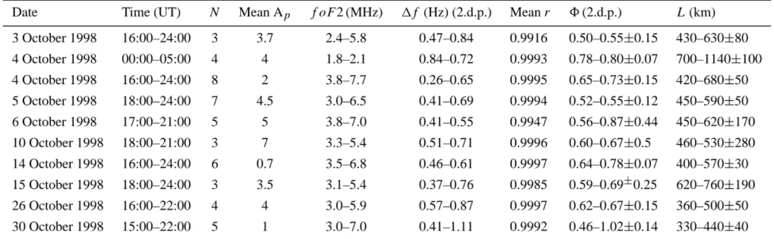
Table 1 is a summary of the resonance feature analysis for the 10 time intervals studied from October 1998. Columns 1–6 show dates of observation and the approximate observa-tion times (in UT) of the resonance features in the magnetic dynamic spectra, the number of harmonics seen, the mean Ap, the range of f0F2 critical frequency values during the interval, and the harmonic spacing (1f ) during these times respectively. Columns 7–9 give model IAR parameters de-rived from data analysis which will be explained later. All except one morning interval from 02:00–06:00 LT on 4 Octo-ber 1998 are night-time observations of increasing harmonic frequencies and spacing, typically starting from 18:00 LT and fading out after 02:00 LT. Generally more harmonics were visible on days when the average Ap during the ob-servation period was low, since the total power in the spectra was lower, making small amplitude signals detectable at the higher frequency end of the spectra despite the drop-off in sensitivity of the magnetometer. The resonance features were observed for longer when the Ap was small; a quiet magne-tosphere is best for observing relatively weak IAR resonance features. This is illustrated in Fig. 8, which is a scatter plot of the duration of the resonance feature observations against the mean Apduring this time. A least squares regression line is plotted, whose product moment correlation coefficient (Pear-son’s r) was good (−0.79), indicating a negative relationship between resonance feature duration and mean Ap.
S. R. Hebden et al.: A quantitative analysis of diurnal evolution 1717
Table 1. Summary of the IAR resonance feature analysis for October 1998. The 2nd column shows the approximate times between which
IAR spectral resonance features were observed in the pulsation magnetometer data from Sodankyl¨a, Finland. The 3rd column gives the number of harmonics that were clearly visible in the dynamic colour spectra. Column 4 shows the average Apindex during the resonance feature observation. The 5th and 6th columns indicate how the f0F2 critical frequency measured by the ionosonde at Sodankyl¨a and the resonance feature spacing varied from the start to finish of the resonance features. Column 7 gives the average product moment correlation coefficient over the resonance feature observations. This is the mean of the hourly correlations between resonance peak frequency and harmonic number. The 8th and 9th columns indicate the range of values of 8 and L calculated for each time interval, and their associated errors.
Date Time (UT) N Mean Ap f oF2 (MHz) 1f (Hz) (2.d.p.) Mean r 8(2.d.p.) L(km)
3 October 1998 16:00–24:00 3 3.7 2.4–5.8 0.47–0.84 0.9916 0.50–0.55±0.15 430–630±80 4 October 1998 00:00–05:00 4 4 1.8–2.1 0.84–0.72 0.9993 0.78–0.80±0.07 700–1140±100 4 October 1998 16:00–24:00 8 2 3.8–7.7 0.26–0.65 0.9995 0.65–0.73±0.15 420–680±50 5 October 1998 18:00–24:00 7 4.5 3.0–6.5 0.41–0.69 0.9994 0.52–0.55±0.12 450–590±50 6 October 1998 17:00–21:00 5 5 3.8–7.0 0.41–0.55 0.9947 0.56–0.87±0.44 450–620±170 10 October 1998 18:00–21:00 3 7 3.3–5.4 0.51–0.71 0.9996 0.60–0.67±0.5 460–530±280 14 October 1998 16:00–24:00 6 0.7 3.5–6.8 0.46–0.61 0.9997 0.64–0.78±0.07 400–570±30 15 October 1998 18:00–24:00 3 3.5 3.1–5.4 0.37–0.76 0.9985 0.59–0.69±0.25 620–760±190 26 October 1998 16:00–22:00 4 4 3.0–5.9 0.57–0.87 0.9997 0.62–0.67±0.15 360–500±50 30 October 1998 15:00–22:00 5 1 3.0–7.0 0.41–1.11 0.9992 0.46–1.02±0.14 330–440±40
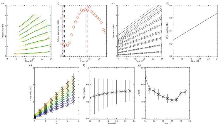
The stages of analysis for each time interval are illustrated in Fig. 9, for 4 October 1998. Panel a) shows the cursor clicked determinations of the harmonic frequencies with time for each polarization. The H, D, RH and LH polarization components are plotted in red, yellow, green and blue respec-tively. Panel b) shows the diurnal variation in the f0F2 crit-ical frequency from the ionosonde at Sodankyl¨a in red dia-monds. Where data is missing or uncertain (most commonly due to absorption in a lower ionospheric layer), the data points are linearly interpolated. For data gaps lasting longer than 5 h, linear interpolation is meaningless and the critical frequency is plotted as 0. The error associated with the criti-cal frequency is 5% where the uncertainty is quantified on the ionosonde data tables, and assumed to be about 10% for lin-early interpolated points. The terminator crossings at ground level and at 100 km altitude above Sodankyl¨a are shown as black and purple dashed lines respectively. The least squares regression lines of the cursor points for each harmonic using all the polarizations are plotted as solid black lines, and their uncertainty (given by the standard deviation of the points) are shown in panel c) as dot-dash lines. On some days, the magnetic field strength of the resonance features vary from one polarization to another, thus the least squares regression lines (see panel c)) through the cursor points (in panels a)) are calculated from less than 4 polarizations. This increases the standard deviation of the points about the least squares re-gression lines, making the experimental error larger in deter-mining the positions of the resonance features. Panel d) is a plot of how the harmonic spacing, 1f , varies with time, cal-culated from the linear functions that describe the harmonic frequency variation with time plotted in panel c).
Scatter plots of the harmonic frequencies (f ) versus har-monic number (N ) were plotted for each hour when the res-onance features were identified. An example of this is given in panel e) of Fig. 9, with error bars that represent the un-certainty in frequency shown in panel c). Least squares re-gression lines through these points are plotted in different colours for each hour going from purple-yellow with increas-ing time. For all of the dates analyzed, all of the gradients of the lines increase with time except those during the post-midnight time interval, which decrease. The same is true for the intercepts, although the flatness of the resonance features observed on 6 October 1998 made any variation in intercept very small. The product moment correlation coefficients (r) for f versus N at any instant in time vary, but they are gener-ally very high (the mean values of r during each time interval analyzed are shown in column 7 of Table 1). For example on 14 October 1998 the average value of r is 0.9997, indicating that there is a near perfect linear relationship between har-monic frequency and harhar-monic number throughout the reso-nance feature time intervals analyzed.
The strong linear relationships between harmonic fre-quency and harmonic number for all of the time intervals that were studied are consistent with a homogeneous cavity model used by Trakhtengerts et al. (2000) for the IAR, which was consequently adopted for interpretation purposes. In this simple model, reflection of Alfv´en waves occurs within the top and bottom layers, and standing waves are set up in the middle layer. For resonance of waves with wave speed vAin a uniform cavity of length L, the frequency f of harmonic
1718 S. R. Hebden et al.: A quantitative analysis of diurnal evolution a) 14 16 18 20 22 24 T ime UT 0 1 2 3 4 5 F re q u e n cy ( H z) b) 5 10 15 20 T ime UT 0 2 4 6 8 C ri tic a l f re q u e n cy ( M H z) c) 14 16 18 20 22 24 T ime UT 0 1 2 3 4 5 F re q u e n cy ( H z) d) 14 16 18 20 22 24 T ime UT 0.0 0.2 0.4 0.6 0.8 S R S s p a ci n g ( H z) e) 0 2 4 6 8 N 0 2 4 6 F re q u e n cy ( H z) f) 14 16 18 20 22 24 T ime UT 0.4 0.6 0.8 1.0 P h a se f a ct o r g) 14 16 18 20 22 24 T ime UT 200 400 600 800 L ( km )
Figure 9. Analysis of the magnetic spectral resonance features seen in pulsation magnetometer data at Sodankylä, Finland on 04/10/98. Panel a) shows the
resonance feature frequency evolution over time defined using method 1 from 4 polarisation components: H (red line), D (yellow), RH (green) and LH (blue). Panel b) shows the diurnal fOF2 critical frequency variation from a co-located ionosonde in red diamonds, with the time of the terminator crossing Sodankylä on the
ground and at 100km altitude in black and purple dashed lines respectively. Panel c) shows least squares regression lines through the harmonic points plotted in panel a), with error margins shown as dot-dashed lines given by the standard deviation of these points. Panel d) plots the function of harmonic spacing with time, as calculated from the harmonics plotted in panel c). Panel e) shows frequency plotted against harmonic number for each hour from 14-23 UT, with least squares regression lines through these points going purple-orange in time. Panels f) and g) show the evolution of wave phase factor and L with time.
Fig. 9. Analysis of the magnetic spectral resonance features seen in pulsation magnetometer data at Sodankyl¨a, Finland on 4 October 1998.
Panel (a) shows the resonance feature frequency evolution over time derived for each polarisation component: north south component (red), east west (yellow), right-handed circular (green) and left-handed circular polarisation (blue). Panel (b) shows the diurnal f0F2 critical frequency variation from a co-located ionosonde in red diamonds. The terminator crossings at ground level and at 100 km altitude above Sodankyl¨a are shown as black and purple dashed lines respectively. Panel (c) shows least squares regression lines through the harmonic points plotted in panel a), with error margins shown as dot-dashed lines given by the standard deviation of these points. Panel (d) plots the function of harmonic spacing with time, as calculated from the harmonics plotted in panel c). Panel (e) is a scatter plot of harmonic frequency plotted against harmonic number for each hour from 14:00–23:00 UT, with least squares regression lines through these points going purple-yellow with increasing time. Panels (f) and (g) show the evolution with time of wave phase factor 8 and effective IAR cavity size, L, respectively.
number N is given by (Polyakov and Rapoport, 1981):
f = (N + 8)vA
2L (1)
where 8 is the wave “phase factor”. This was originally introduced as a constant value of 1/4. (These authors also used (l+h) instead of L in Eq. (1), where H is the thickness of the bottom side of the ionosphere and l is the scale of the electron density exponential decay in the upper ionosphere.) The value of 8 may be controlled by the reflection coefficient at the lower IAR boundary, Rlower, which can be written in terms of r=6ω/6pand is given by (Lysak, 1991):
Rlower = r −1
r +1 (2)
where 6ω the wave conductance 6ω=1/µ0vI AR and 6p is the integrated Pedersen conductivity. If there is a wave node (for high ionospheric conductivity) at the lower boundary of the IAR with the reflection coefficient Rlower∼−1, we ex-pect the value of 8 to be half integer. For a wave antinode
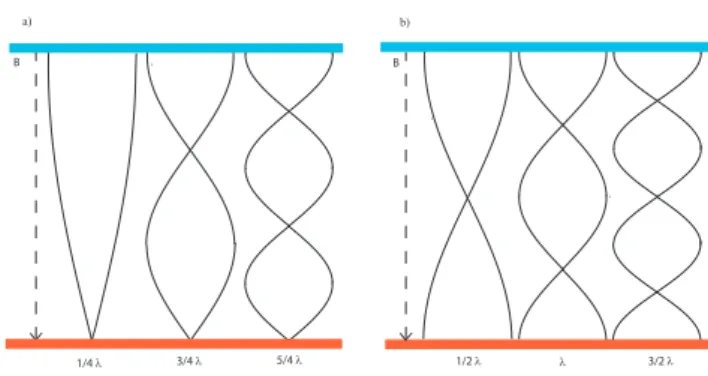
(low ionospheric conductivity) with Rlower∼1, 8 will be in-teger (Lysak, 1991). There is always an antinode at the upper IAR boundary. The high and low conductivity cases are il-lustrated in panels a) and b) respectively of Fig. 10. This diagram shows the first 3 IAR eigenmodes in each case, and how many fractions of a wavelength are set up in the IAR cavity of length L.
The gradient of a least squares regression line for f against N at an instant in time gives, according to Eq. (1), K=vA/2L, and the intercept on the f -axis at an instant in time gives Kφ. Therefore, the intercept divided by the gradient of the least squares regression line at any instant in time gives 8. The variation of ˆO with time on 4 Octo-ber 1998 is plotted in panel f) of Fig. 11, with error bars given by the combined uncertainty in the intercepts and slopes of the f against N plot at each point in time (i.e. (1 8/8)2=(1K8/K8)2+(1K/K)2). Column 8 of Table 1 shows the range of values taken by 8 for each time inter-val studied and the mean error in these inter-values. The inter-values of 8 obtained in this study ranged between 1/2 and 1 which was expected from theory, if 8 represents the fraction of a
S. R. Hebden et al.: A quantitative analysis of diurnal evolution 1719 quarter wavelength that forms a standing wave in addition
to the integer number of half wavelengths necessary for cav-ity resonance. Thus 8 acted as a consistency check on the model.
The average value of 8 from all of the time intervals an-alyzed is 0.61, which is close to the value expected for high conductivity at the lower boundary. The highest value for 8 of 1.02±0.26 occurred on 30 October 1998 which dropped more dramatically than for any other time interval, ending in the lowest value for 8: 0.46±0.10. During this interval the f0F2 frequency underwent the largest change, dropping from 7 MHz to 3 MHz, and the fOEdropped more than most intervals, from 3.5 MHz to 1.75 MHz. This means that the plasma density in the E and F regions dropped, reducing the Pedersen conductivity. However, from the analysis, 8 went from integer (expected for low conductivity) to half integer (high conductivity), counter to what is expected from the-ory. Preliminary comparisons of the lower boundary reflec-tion coefficient (calculated using electron density and tem-perature data from the EISCAT incoherent scatter radar) on 2 days in October 1998 did not show a consistent picture ei-ther. Thus the value of 8 obtained with this simple modelling interpretation of IAR resonance features cannot be used to infer the E region conductivity.
The variation of L with time can also be calculated if the variation of vA with time is known. This is provided by hourly estimates of the f0F2 critical frequency from the ionosonde at Sodankyl¨a, which measures the peak plasma density in the F2-layer, and so determines how the density in the IAR varies in time, and hence how the Alfv´en speed vA in the IAR varies with time. Since K is a function of vAand L, the variation of L with time is given by vA/2K.vA was calculated from the f0F2 critical frequency (in MHz) since ionosondes measure the electron number density (N e) of the F2 layer directly (N e=1.24×10¹⁰×f0F22):
vA= B fOF2 p 1.24 × 10¹⁰µ0m i (3) where the average mass loading of the field line in the IAR, mi is assumed to be 24.7 a.m.u. (calculated using the IRI model, taking and average over the height range of 100– 300 km altitude with appropriate ionospheric conditions in-put) and B is the average geomagnetic field strength at these altitudes. This is expected to yield underestimated values of L,because the effective IAR density that affects the trapped Alfv´en waves is smaller than the density of the F2 peak. The calculated variations in L (shown in panel g) for 4 Octo-ber 1998) simply indicate the variation in the scale size of the IAR with time. The error bars shown in panel g) are given by the combined uncertainty in the gradients of the f against N plots and the f0F2 frequency at each point in time (i.e. (1L/L)2=(1K/K)2+(1fOF2/fOF2)2).
Column 9 of Table 1 summarises the variation of L for each time interval studied. The average value of L from all of the time intervals is 530 km. The maximum variation of Loccurred in the morning time interval of 4 October 1998, with L increasing from 700–1140±100 km. The minimum
B B
a) b)
1/4 l 3/4 l 5/4 l 1/2 l l 3/2 l
Figure 10. In both panels the lower red rectangle represents the lower IAR boundary and the blue rectangle represents the upper IAR boundary. The background magnetic field is directed downwards for high latitude northern hemisphere regions. Panel a) shows the perpendicular electric field for the first 3 eigenmodes for the case of a high conductivity ionosphere with a node at the lower IAR boundary. Panel b) shows the first 3 standing wave modes in the case of a low conductivity ionosphere with an antinode at the lower IAR boundary.
Fig. 10. Diagram showing an Alfv´en wave’s perpendicular
elec-tric field for the first 3 eigenmodes trapped in the IAR for the high conductivity ionosphere (panel (a)) and low conductivity (panel
(b)) ionosphere. The lower red rectangles represent the lower IAR
boundary and the blue rectangle represents the upper IAR boundary. The background magnetic field is directed downwards for the high latitude northern hemisphere regions. Panel a) for a high conduc-tivity ionosphere shows a node at the lower IAR boundary. Panel b) for a low conductivity ionosphere displays an antinode at the lower IAR boundary. 0.2 0.4 0.6 0.8 1.0 K (m s-1 km-1) 4.0•10 5 6.0•10 5 8.0•10 5 1.0•10 6 1.2•10 6 1.4•10 6 vA (m s -1)
Figure 11. Scatter plot summarizing the analysis results. The horizontal axis
is gradient, K, of the lines of best fit of f against N at each hour for the IAR resonance features. The vertical axis is Alfvén velocity calculated directly from the electron density given by the foF2 hourly data, assuming that the mean ion mass in the IAR is given by the mean in the F region ~ 24.7 a.m.u. The gradient of the least squares regression line through these points gives 2 L, where L = 530 km is the mean IAR scale height for all of the 10 intervals of IAR resonance features that were analyzed in detail. The colour of the stars varies according to date, going from black-red-yellow-green-blue with chronological order.
Fig. 11. Scatter plot of the IAR resonance feature analysis from
Sodankyl¨a during October 1998, where the colour of the stars vary according to date, going from red to blue with chronological order. On the horizontal axis is plotted gradient, K, of the lines of best fit of f against N at each hour for the IAR resonance features. The vertical axis is Alfv´en velocity calculated directly from the electron density given by the fOF2 hourly data, assuming that the mean ion mass in the IAR is given by the mean in the F region ∼24.7 a.m.u. The gradient of the least squares regression line through these points gives 2 L, where L=530 km, the mean IAR scale height for all of the 10 intervals of IAR resonances that were analysed in detail.
variation occurred on 10 October 1998, although the error margin is large for this day; L varies from 460–530±280 km. In summary, a typical scale size for the IAR is ∼500 km, which is 2–3 times the typical plasma scale height in the ionosphere.
These results for L can also be explained with the aid of the scatter diagram shown in Fig. 11. The gradients, K, of all of the hourly lines of best fit of f against N are plotted against the hourly values for vA calculated di-rectly from the f0F2 critical frequencies and assuming that
1720 S. R. Hebden et al.: A quantitative analysis of diurnal evolution mi=24.7 a.m.u. The different coloured stars symbolize data
for different days. The gradient of the least squares re-gression line through all of the points gives 2L, where L=530 km±150 km, the average scale size and standard de-viation of the IAR respectively for all 10 time intervals of IAR resonance features studied. The red stars represent data for the sole post-midnight interval (just after dawn) on 4 October 1998 when the f0F2 frequency rapidly increased, hence making the IAR size increase rapidly (as described above).
This study of IAR resonance features has shown that they are commonly observed in the quiet-time background noise from the Sodankyl¨a pulsation magnetometer; in Octo-ber 1998 multiple harmonics were observable for about 66 h, most commonly after 16:00 UT which is 1–2 h after sunset, and sometimes into the early hours of the morning, 1–2 h af-ter sunrise. The longest inaf-terval of resonance features lasted for 13 h from 16:00 UT on 3 October 1998 until 05:00 UT on 4 October 1998. The harmonics are quasi-evenly spaced at all times, as shown from the strong linear relationships be-tween harmonic frequency and harmonic number.
The frequency of each harmonic varies with time of day very slowly and systematically, on average the harmonic spacing c increased by ∼0.06 Hz per hour towards midnight and decreased by 0.02 Hz per hour post midnight. The rela-tive changes in the fundamental frequency over the time in-tervals were calculated, with an average change over all the time intervals of 52%. The relative change in the effective cavity size, L was calculated; whose average is 32% over a time interval of a few hours. This is low compared to the relative change in vA of 61% due to the diurnal varia-tion of the plasma density in the F2 layer. This indicates that the diurnal evolution of the IAR harmonic frequencies is chiefly caused by the changing Alfv´en velocity in the F2 region of the ionosphere. The Alfv´en velocity is proportional to fOF2−1, so as the fOF2 frequency drops rapidly towards midnight and rises more slowly in the morning (see Fig. 9 panel b)) the IAR spectral resonance features do the con-verse. These results support the results published by Belyaev et al. (1990) who used data from a mid-latitude magnetome-ter station and an ionosonde. It was also demonstrated quali-tatively by Belyaev et al. (1999) using 2 days of data from a high-latitude magnetometer and electron densities variations derived from EISCAT incoherent scatter radar data. How-ever it is not only the Alfv´en velocity that determines the evolution of the IAR eigenfrequencies but also the size of the IAR cavity, L,as discussed by Odzimek, (2004). Yah-nin et al. (2003) also calculated the long-term variations of a parameter they termed L characterizing the scale of electron density decrease above the F-layer maximum at Sodankyl¨a similar to L in this paper but without estimating the average ion mass miin the IAR. They used ionosonde f0F2 measure-ments and SRS frequency interval 1f from magnetometer data averaged over 3-h intervals. The parameter showed sea-sonal variability, peaking in summer months where data was available for nighttime time intervals. During October 1998 the diurnal variation of L was not more than 30%, which
agrees with the results of the present study. Thus, L is a rela-tively stable parameter; the diurnal evolution of the harmonic frequencies is most strongly dependent on Alfv´en velocity, since IAR size is less variable.
The relative change in 8 calculated for the time intervals of this study was very low, at 20%. With reference to Eq. (1), the values of 8 obtained in this study ranged between 1/2 and 1, thus acted as a consistency check on the model. It is believed that 8 determines the fraction of a quarter wave-length that forms a standing wave in addition to the integer number of half wavelengths necessary for cavity resonance. The value of 8 depends on whether the wave reflection at the lower boundary is a node or an antinode, or something in between. A preliminary comparison of the diurnal varia-tion of 8 and the ionospheric conductivity/lower boundary reflection coefficient was made using 3 h of EISCAT inco-herent scatter radar data available during October 1998 when IAR resonance features were observed. However, these re-sults were not conclusive and further investigation is neces-sary on other days when IAR resonance features and radar data coincide.
4 Conclusion
Spectral IAR resonance features were successfully identified in pulsation magnetometer data from Sodankyl¨a, Finland on 13 out of 30 days in October 1998. The variations in the res-onance frequencies over time were quantified and analysed in detail for 10 days, using dynamic colour spectra of the data and an interactive cursor clicking technique. Strong lin-ear relationships between harmonic frequency and harmonic number for all of the time intervals studied enabled a homo-geneous cavity model for the IAR to be adopted to analyze the data further. When the variation of the f0F2 region at the same location was taken into account, the detailed anal-ysis of magnetic resonance features yielded a parameter that describes the effective size of the IAR, L. During the time in-tervals studied, the average variation of L over the time inter-vals studied was 32%, whereas the Alfv´en velocity calculated electron density in the F2 region of the ionosphere varied by 61%. Thus the IAR cavity is fairly stable over the 3–10 h time intervals studied and over the 30 day interval over which IAR resonance features were analyzed during October 1998. Therefore the diurnal evolution of the IAR eigenfrequencies is caused, in the main, by the changing density of the IAR throughout the day, confirming previous studies of IAR reso-nance features and local IAR parameters (Demekhov, 2000, Odzimek, 2004, Yahnin et al, 2003). Another IAR parameter was derived from the analysis of the IAR resonance features associated with the phase matching structure of the stand-ing waves in the IAR, termed the phase factor, 8. 8 varied over the time intervals studied by 20% on average, possibly due to changing ionospheric conductivity, although the re-sults were inconclusive due to a lack of incoherent radar data when IAR resonance features are observed. The value of 8 is thought to depend on whether the wave reflection at the
S. R. Hebden et al.: A quantitative analysis of diurnal evolution 1721 lower boundary is a node or an antinode, or something in
be-tween. Further investigation is necessary on other days when IAR resonance features and radar data coincide to determine the relationship between 8 and the lower IAR boundary re-flection coefficient.
Acknowledgements. The Editor in chief thanks A. Yahnin and
an-other referee for their help in evaluating this paper.
References
Belyaev, P. P., Bosinger, T., Isaev, S. V., and Kangas, J.: First ev-idence at high latitudes for the Ionospheric Alfv´en resonator, J. Geophys. Res., 104(A3), 4305–4317, 1999.
Belyaev, P. P., Polyakov, S. V., Rapoport, V. O., and Trakhtengerts, V. Yu.: Discovery of resonance structure in the spectrum of atmo-spheric electromagnetic background noise in the range of short-period geomagnetic pulsations, Doklady Akademii Nauk SSSR, 297, 840–846, 1987.
Belyaev, P. P., Polyakov, S. V., Rapoport, V. O., and Trakhtengerts, V. Yu.: Izu. VUZov, Radiofizika, XXXII(N6), 1989.
Belyaev, P. P., Polyakov, S. V., Rapoport, V. O., and Trakhtengerts, V. Yu.: The Ionospheric Alfv´en resonator, J. Atmos. Terr. Phys., 52, 781–788, 1990.
Belyaev, P. P., Polyakov, S. V., Ermakova, E. N., and Isaev, S. V.: Solar cycle variations in the ionospheric Alfv´en resonator 1985– 1995, J. Atmos. Terr. Phys., 62, 239–248, 2000.
Carlson, C. W., Pfaff, R. F., and Watzin, J. G.: The Fast Auroral SnapshoT mission, Geophys., Res., Lett., 25(12), 2013–2016, 1998.
Cash, S. R., Davies, J. A., Kolesnikova, E., Robinson, T. R., Wright, D. M., Yeoman, T. K., and Strangeway, R. J.: Electron acceler-ation observed by the FAST satellite within the IAR during a 3 Hz modulated EISCAT heater experiment, Ann. Geophys., 20, 1499–1507, 2002,
SRef-ID: 1432-0576/ag/2002-20-1499.
Demekhov, A. G., Belyaev, P. P., Isaev, S. V., Manninen, J., Tu-runen, T., and Kangas, J.: Modelling the diurnal evolution of the resonance spectral structure of the atmospheric noise background in the Pc1 frequency range, J. Atmos. Terr. Phys., 62, 257–265, 2000.
Hickey, K., Sentman, D. D., and Heavner, M. J.: Ground-based observations of ionospheric Alfv´en resonator bands, Fall meeting AGU, A22C-08, 1996.
Kolesnikova, E., Robinson, T. R., Davies, J. A., Wright, D. M., and Lester, M.: Excitation of Alfv´en waves by modulated HF heating of the ionosphere, with application to FAST observations, Ann. Geophys., 20, 57–67, 2002,
SRef-ID: 1432-0576/ag/2002-20-57.
Lynn, P. A.: An Introduction to the Analysis and Processing of Sig-nals, Macmillan, 1984.
Lysak, R. L.: Feedback instability of the Ionospheric Resonant cav-ity, J. Geophys. Res., 96(A2), 1553–1568, 1991
Odzimek, A.: Numerical estimate of the spectral resonance struc-ture frequency scale of natural ULF magnetic field, Stud. Geo-phys. Geod., 48, 647–660, 2004.
Polyakov, S. V.: On properties of an ionospheric Alfv´en resonator, in Symposium KAPG on Solar-Terrestrial Physics, vol. III, 72– 73, Nauka, Moscow, 1976.
Polyakov, S. V. and Rapoport, V. O.: Ionospheric Alfv´en resonator, Geomagnetism and Aeronomy, 21 (5), 816–822, 1981.
Rishbeth, H., and Williams, P. J. S.: The EISCAT Ionospheric Radar: the System and its Early Results, Q. Jl. R. astr. Soc., 26, 478–512, 1985.
Robinson, T. R., Strangeway, R. J., Wright, D. M., Davies, J. A., Horne, R. B., Yeoman, T. K., Stocker, A. J., Lester, M., Rietveld, M. T., Mann, I. R., Carlson, C. W., and McFadden, J. P.: FAST observations of ULF waves injected into the magnetosphere by means of modulated RF heating of the auroral electrojet, Geo-phys. Res. Lett., 27, 3165–3168, 2000.
Stubbe, P., Kopka, H., Lauche, H., Reitveld, M. T., Brekke, A., Holt, O., Jones, T. B., Robinson, T. R., Hedberg, A., Thide, B., Crochet, M., and Lotz, H. J.: Ionospheric modification experi-ments in northern Scandinavia, J. Atmos. Terr. Phys., 44, 1025– 1041, 1982.
Trakhtengertz, V. Y., Belyaev P. P., Polyakov, S. V., Demekhov, A. G., and Bosinger, T.: Excitation of Alfv´en waves and vortices in the ionospheric Alfv´en resonator by modulated powerful radio waves, J. Atmos. Terr. Phys., 62, 267–276, 2000.
Wright, D. M., Davies, J. A., Yeoman, T. K., Robinson, T. R, Cash, S. R., Kolesnikova, E., Lester, M., Chapman, P. J., Strangeway, R. J., Horne, R. B., Rietveld, M. T., and Carlson, C. W.: Detec-tion of artificially generated ULF waves by the FAST spacecraft and its application to the “tagging” of narrow fluw tubes, J. Geo-phys. Res., 108(A2), 1090, 2003.
Yahnin, A. G., Semenova, N. V., Ostapenko, A. A., Kangas, J., Manninen, J., and Turunen, T.: Morphology of the spectral res-onance structure of the electromagnetic background noise in the range of 0.1–4 Hz at L=5.2, Ann. Geophys., 21, 779–786, 2003,