The occurrence frequency of upward ion beams in the auroral zone as a function of altitude using Polar/TIMAS and DE-1/EICS data

HAL Id: hal-00317173

https://hal.archives-ouvertes.fr/hal-00317173

Submitted on 1 Jan 2003

HAL is a multi-disciplinary open access

archive for the deposit and dissemination of

sci-entific research documents, whether they are

pub-lished or not. The documents may come from

teaching and research institutions in France or

abroad, or from public or private research centers.

L’archive ouverte pluridisciplinaire HAL, est

destinée au dépôt et à la diffusion de documents

scientifiques de niveau recherche, publiés ou non,

émanant des établissements d’enseignement et de

recherche français ou étrangers, des laboratoires

publics ou privés.

The occurrence frequency of upward ion beams in the

auroral zone as a function of altitude using

Polar/TIMAS and DE-1/EICS data

P. Janhunen, A. Olsson, W. K. Peterson

To cite this version:

P. Janhunen, A. Olsson, W. K. Peterson. The occurrence frequency of upward ion beams in the

auroral zone as a function of altitude using Polar/TIMAS and DE-1/EICS data. Annales Geophysicae,

European Geosciences Union, 2003, 21 (10), pp.2059-2072. �hal-00317173�

Annales

Geophysicae

The occurrence frequency of upward ion beams in the auroral zone

as a function of altitude using Polar/TIMAS and DE-1/EICS data

P. Janhunen1, A. Olsson2, and W. K. Peterson3

1_{Finnish Meteorological Institute, Geophysical Research, Helsinki, Finland}

2_{Swedish Insititute of Space Physics, Uppsala Division, Uppsala, Sweden}

3_{LASP, University of Colorado, Boulder, Colorado, USA}

Received: 12 September 2002 – Revised: 16 January 2003 – Accepted: 6 February 2003

Abstract. We study the occurrence frequency of upward

au-roral ion beams as a function of altitude using three years of Polar/TIMAS ion data combined with 11 years of DE-1/EICS ion data, in order to reach a complete altitude cover-age between 5000 and 30 000 km. The most interesting result is that there is a peak in ion beam occurrence frequency and

invariant energy flux and invariant particle flux at ∼3 RE

ra-dial distance. The peak exists at about the same altitude in both the evening and midnight MLT sectors. No solar cycle effects are found. We suggest that the peak could be due to a

preferred altitude of auroral potential structures at ∼3 RE. To

substantiate the suggestion, we also present a simple Monte Carlo simulation of ion beams. Another result is that the ion beam occurrence frequency and invariant (mapped to iono-spheric altitude) energy and particle fluxes increase in the

radial distance range 4–6 RE, suggesting that wave heating

processes may take place in this altitude range.

Key words. Magnetospheric physics (auroral phenomena;

magnetosphere-ionosphere interactions) – Space plasma physics (charged particle motion and acceleration)

1 Introduction

Discrete auroral arcs are associated with inverted-V type ac-celerated electron precipitation (Frank and Ackerson, 1971). The electron acceleration takes place in an upward parallel electric field residing at ∼3000–11 000 km altitude range (the altitude depends on season). The parallel electric field be-longs to the bottom part of a U-shaped potential structure. Besides accelerating electrons downward, the parallel elec-tric field also accelerates ionospheric ions upward, forming upgoing ion beams above the bottom of the potential struc-ture (McFadden et al., 1998). The mean energy of the beam ions is expected to agree at least approximately with the mag-nitude of the potential drop, although care in interpretation is needed because different species are energized differently

Correspondence to: A. Olsson (ao@irfu.se)

(M¨obius et al., 1998). Other closely related auroral phenom-ena are ion conics (Kondo et al., 1990), but they are related to perpendicular wave heating and thus do not give infor-mation about the potential structure (Andr´e and Yau, 1997). Indications of a combination of parallel acceleration and per-pendicular heating (called bimodal acceleration by Klumpar et al., 1984) have also been found in the form of conics el-evated in energy (Miyake et al., 1996). Although this much is known about discrete auroral arc formation at low altitude, important questions remain open, such as what is the mor-phology of the potential structure at higher altitude and what is the physical energy transfer mechanism maintaining the whole potential structure.

Studying the altitude dependence of ion beams is thus one way to approach the physical question of what causes and maintains the inverted-V machinery of auroral electron ac-celeration, and one which has not been widely pursued yet. However, some studies on the topic have been done. The al-titude dependence of ion beams was studied statistically by Yau et al. (1984) and Kondo et al. (1990), both using DE-1 data (8000–24 000 km altitude range). The Yau et al. (1984) study uses 1981–82 data while Kondo et al. (1990) use 1981–

86. For high Kpvalues, a minimum in ion beam occurrence

frequency for both oxygen and hydrogen was found at around 16 000 km altitude (except for energies less than 1 keV for which the occurrence frequency was monotonically increas-ing as a function of altitude). Studyincreas-ing this phenomenon fur-ther is one of the motivations for the present study.

In order to obtain the maximum information that ion beam altitude dependence can give about auroral accelera-tion mechanisms, one has to study the altitude dependence also as a function of magnetic local time (MLT) and

invari-ant latitude (ILAT), as well as for different Kp, solar

illu-mination and solar cycle phase conditions. We now briefly review previous results for ion beam dependence on these parameters and put them into the context of other auroral processes. Ion beam occurrence frequencies as a function of MLT and integrated over altitude appeared in Gorney et al. (1981), Fig. 3, and Yau et al. (1985), Fig. 8. The maximum

number of fluxes in O+_{ion beams were found to occur in the} pre-midnight sector, which is probably due to the fact that inverted-V phenomena are the most common there (Lin and Hoffman, 1979). Statistical plots of the ILAT dependence of the occurrence frequency (integrated over altitude) appeared in Yau et al. (1985). The low energy ion beam ILAT versus MLT dependence closely followed the ILAT versus MLT de-pendence of the auroral oval, which is another indication that ion beams are closely associated with inverted-V electron

ac-celeration. Regarding Kp dependence (Fig. 5 of Yau et al.

(1985) and Fig. 8 of Kondo et al. (1990)), it was found that

the ion fluxes increase as a function of Kp, which probably

reflects the general increase in auroral processes with Kp.

Using one year of TIMAS data it has also been found that ion beams below 10 000 km occur ∼3 times more often dur-ing wintertime than durdur-ing summertime (Collin et al., 1998). This probably reflects the fact that during summertime, po-tential structures and their associated ion beams often reside at higher altitude, because of higher underlying ionospheric plasma density and thus were more often beyond the upper altitude limit of this study. What is missing in these stud-ies is an altitude dependence together with the other previous parameters. This is the subject of the present paper.

In this paper we study the ion beams statistically as a func-tion of altitude using two different ion instruments, TIMAS and EICS, from two satellites, Polar and DE-1, respectively. The main reason for selecting Polar is the fact that it covers all altitudes above 5000 km, up to and exceeding 30 000 km which we set as the upper limit of our study. The TIMAS in-strument on board Polar suffered a high-voltage breakdown on 8 December 1998 and thus the altitude coverage is incom-plete. We use DE-1/EICS to complete the altitude coverage. DE-1/EICS is similar to TIMAS, except that the time and energy resolutions are somewhat inferior. The main new top-ics that we will study are the statistical altitude profile of ion beam occurrence frequency up to 30 000 km, and how the al-titude profile of ion beams depends on MLT, ILAT, etc. This paper is part of a larger ongoing effort where we look at the altitude dependence of several inverted-V related phenom-ena, such as density cavities, potential structures, broad-band electrostatic waves and electron anisotropies. The overarch-ing goal is to study the physical mechanisms of electron ac-celeration in discrete auroral arcs. For this purpose one needs information about the plasma physical processes in a wide al-titude range in auroral flux tubes.

Investigation of counterstreaming ion beams lead Sagawa et al. (1987) and Horita et al. (1987) to infer the exis-tence of a downward directed electric field at high altitudes. More specifically, Janhunen et al. (1999) and Janhunen and Olsson (2000) proposed that the low-altitude U-shaped

po-tential contours often close below 4–5 RE radial distance,

forming an “O-shaped” potential. Support for the idea has later come from simulations (Janhunen and Olsson, 2002; Janhunen et al., 2003), Polar/FAST conjunctions (Janhunen et al., 2001), and studies of hemispherical conjugacy of au-roras (Hallinan and Stenbaek-Nielsen, 2001). The effect of a closed negative potential structure on ion beams is that the

beam which is energized at the bottom of the structure should become decelerated at the top of the structure. In a statistical study, time histories of individual ion beams surely cannot be followed, but the phenomenon should be seen as a reduction of the ion beam occurrence frequency at the closure altitude of the potential contours. Testing the closed potential struc-ture hypothesis from the ion beam point of view is one of the motivations of the paper.

2 Instrumentation and data analysis

We use Polar/TIMAS for covering the altitude ranges 5000– 10 000 and 20 000–32 000 km during 1996–1998 (Shelley et al., 1995). TIMAS suffered a high-voltage breakdown in 8 December 1998 and experienced a loss of telemetry for portions of 1999, 2000 and 2001. Although TIMAS reiniti-ated routine operations on 30 March 2001, the high-voltage breakdown of 1998 resulted in a loss of sensitivity that makes intercomparisons of statistical databases obtained before and after 8 December 1998 too challenging. We chose not to use TIMAS data acquired after 8 December 1998 in this analysis. This makes the altitude coverage of TIMAS incomplete: The EICS instrument on board DE-1 made measurements dur-ing 1981–1991, coverdur-ing altitudes between 8000–23 000 km (Shelley et al., 1981). Using both instruments together we can thus obtain a complete altitude coverage from 5000 km to 30 000 km.

In order to be able to use Polar/TIMAS and DE-1/EICS in the same statistics, careful intercalibration is necessary. This will be addressed in Sect. 2.4 (“Polar/TIMAS and DE-1/EICS intercomparison”).

2.1 Data sets

The Polar/TIMAS instrument produces the differential

en-ergy flux for all pitch angles and energies with 15◦pitch

an-gle bins and 28 logarithmically spaced energy steps between 15 eV and 33 keV every two satellite spins (about 12 s). Be-fore June 1996 the upper energy limit was 25 keV, however. The data files used in this study are version 2 high resolution files from the online database of instrument data from many satellites provided by NASA on the CDAWeb site. The DE-1/EICS instrument is very similar to Polar/TIMAS. However, the time resolution of the CDAWeb data files we are using is 16 spins (96 s, i.e. an 8 times lower time resolution than for Polar/TIMAS) and also the energy range is more restricted than TIMAS (10 eV to 17 keV). Our method for finding ion beams requires at least 2 energy channels above the peak en-ergy; thus, the maximum peak energy with DE-1/EICS is 10 keV. In order to compare the data sets with the same res-olution and restrictions, the energy range of TIMAS is ad-justed to the capabilities of EICS, and each EICS data point is replicated 8 times to match Polar/TIMAS time resolution. The data sets we are using are the best that exist from these instruments. The only compromise in the data quality

in these sets is that gyrotropy has been assumed throughout, but this is no problem in the present study.

After this paper was written, an error was noticed in Po-lar/TIMAS telemetry processing which may affect the day-side flux values in the 10–14 MLT range. Consequently, the flux values in this MLT range appearing in Figs. 8 and 9 be-low may be slightly in error. No conclusions are drawn in this paper concerning this MLT range.

2.2 Finding ion beams

We identify the ion beams as energy-angle structures by the following method based on Gaussian fitting. Ion beams are usually defined as maxima in phase space density, but we choose to define them as peaks in the differential energy flux. Let F (E, θ ) denote the measured differential energy flux, where E is the energy and θ is the pitch angle. Upward ion beams are maxima of F (E, θ ) appearing close to θ = π for the Northern Hemisphere (for the Southern Hemisphere they appear close to θ = 0). Particulary at higher altitude they are often superposed with a smooth background which is almost symmetric in the up/down direction. For each en-ergy step, to separate the background we first subtract the downgoing part from the upgoing part and replace possible negative values by zero after subtraction. We then find all local maxima along θ = π . We consider only maxima that exceed the background by at least 50%. After locating the maximum, the 2-D region in energy and pitch angle around the maximum which belongs to the same ion beam is found. The criteria used here are such that only values that exceed the local background flux by at least 30% are eligible, and the values must be decreasing as one moves away from the maximum. We also require that the differential energy flux

is at least 105cm−2s−1sr−1. A Gaussian function in energy

and pitch angle is then fitted to the maximum region. If the chi-squared of the fit is larger than 1, the fit is rejected. The energy and number fluxes belonging to the maximum region are then computed, scaled by particle flux conservation in a magnetic flux tube to ionospheric altitude and then saved. In the scaling to ionospheric altitude the value of the magnetic field is needed; this is taken from the Polar/MFE, if available, otherwise, the dipole model is used. In the rare event of hav-ing several eligible local maxima in energy, we select the one with the largest number flux. The processing of TIMAS and EICS data is identical except for the different energy grids.

We use several criteria to protect ourselves against differ-ent types of data errors. Passages of data with known instru-ment errors are removed. A data point is excluded if the inte-grated invariant energy flux (“invariant” means that the

quan-tity is scaled to ionospheric altitude) exceeds 104mW m−2

or if the invariant number flux exceeds 1014m−2s−1. These

values are too high to be realistic (physical energy fluxes

val-ues may reach a few hundred mW m−2 at most) and must

correspond to erroneous flux values. Between 1 April 1996 and 8 December 1998, Polar/TIMAS had 23.9 days worth of valid nightside auroral crossing data (ILAT = 65. . .74) and 27 days worth of missing data. The number of bad data

points was only 2 (corresponding to total time 24 s). For DE-1/EICS, the percentage of bad data points is 0.9% and the total amount of nightside auroral zone time is 59 days. By bad data, here, we mean times when the instrument was on and produced data, but the numbers produced do not make physical sense (e.g. were identically zero).

We limit ourselves only to invariant energy fluxes above

0.2 mW m−2 and to ion beam energies in the range from

0.5 keV to 10 keV. There are plenty of ion beams also below 0.5 keV but we shall not include them in this study because we are primarily interested in those inverted-V phenomena that relate to visible auroral arcs whose accelerating poten-tials are of the order of 0.5–1 keV or more. As mentioned above, by invariant energy flux and invariant particle flux we mean that the quantities are projected to the ionospheric level. No distinction between ion species is made. A further condition that we use is that the integrated ion energy flux must be upward at the time of the ion beam, otherwise, the beam is rejected.

2.3 Computation of occurrence frequencies

We want to compute the ion beam occurrence frequency as a function of different variables, among which are the radial distance R, the invariant latitude (ILAT), the magnetic local

time (MLT), the Kpindex value and solar illumination

condi-tion (i.e. whether the ionospheric footpoint is illuminated or not). We do not have enough orbital coverage to obtain the occurrence frequency in the whole five-dimensional array; however, in any event, it would not be practical to plot. In-stead, we typically display the dependence of the occurrence frequency on one of the important parameters, as a function of radial distance and averaged over all ILAT. There are, in principle, two ways to gather the statistics: (1) one puts all data points in the radial bin together and computes the occur-rence frequency for them, (2) one calculates the occuroccur-rence frequency separately for each ILAT bin and computes the arithmetic average of the occurrence frequencies. Method (1) yields longer data vectors and thus smaller statistical un-certainties, but is vulnerable to possibly nonuniform orbital coverage in ILAT. Method (2) does not require uniform ILAT coverage, but gives larger statistical uncertainties if at least one of the ILAT bins contains a significantly smaller

num-ber of data points than the other bins. If fi is the occurrence

frequency in the ith ILAT bin and σ_i2is the corresponding

variance, the standard deviation of the whole radial bin is given by (1/n)

q P

iσi2, where n is the number of ILAT bins

(9 in our case).

We chose to use method (2) in this paper, with the addi-tional assumption that if one of the ILAT bins has less than 100 measurements, it is dropped from the statistics, so that it does not contribute to the total standard deviation.

2.4 Polar/TIMAS and DE-1/EICS intercomparison

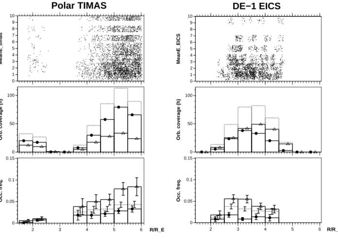
The top panel of Fig. 1 shows all ion beams between 0.5 and 10 keV as a function of radial distance R and beam peak

0 1 2 3 4 5 6 7 8 9 10 MeanE_timas 0 50 100 Orb. coverage (h) 2 3 4 5 6 _{R/R_E} 0 0.05 0.1 0.15 Occ. freq.

Polar TIMAS

Sunlit

DE−1 EICS

Fig. 1. Polar/TIMAS (left), DE-1/EICS (right). Top: All detected 0.5–10 keV beams as a function of radial distance R (RE) and beam

peak energy. Middle: Hours spent by the instrument in each bin. Bottom: Occurrence frequency of ion beams (number of points in each bin divided by the number of 12-s samples coming from the bin, averaged over ILAT). Small Kp(≤ 2) shown by filled circles, large Kp(> 2) by

triangles. Dotted line is both Kps put together. All nightside MLT sectors (18–06) are included and the satellite footpoint is Sun-illuminated.

The method of calculating the error bars is explained in the text. The ILAT range is 65–74.

Table 1. TIMAS and EICS high Kpion beam occurrence frequency when footpoint is sunlit

MLT 18–22 MLT 22–02 MLT 02–06 TIMAS 2–2.5 RE 0.016 ± 0.01 -

-EICS 2–2.5 RE 0.022 ± 0.011 -

-TIMAS 4–4.5 R_E 0.056 ± 0.022 0.044 ± 0.025 0.016 ± 0.014 EICS 4–4.5 RE 0.058 ± 0.025 0.042 ± 0.02 0.009 ± 0.01

energy for conditions where the satellite ionospheric foot-point is sunlit. The left panel shows TIMAS results and the right panel shows EICS. Since the peak energy is quantized to one of the detector energy channel center energies, in or-der to ease plotting, a uniform random number in the range

−0.5...0.5 keV has been added to the ordinate of each data

point. Since TIMAS files have an 8 times higher time res-olution than EICS, each EICS point is replicated 8 times in the upper right panel of Figs. 1 and 2 to make the number of TIMAS and EICS points mutually comparable. Comparison of the left and right panels of Fig. 1 shows that the resulting occurrence frequencies agree relatively well in those altitude

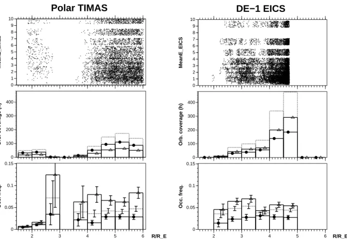
bins where both instruments have coverage. Figure 2 shows the corresponding result for conditions where the satellite ionospheric footpoint is in darkness. Also, here, TIMAS and EICS ion beam occurrence frequencies are in agreement in those altitude bins where both instruments have proper cov-erage.

The error bars shown in all figures of this paper correspond to the standard deviations obtained by assuming that all data points within one auroral zone crossing of each bin are fully correlated. The method is as follows. For a given bin, assume there are N data points, n ion beams and K auroral zone crossings. The occurrence frequency f is given by f = n/N

0 1 2 3 4 5 6 7 8 9 10 MeanE_timas 0 100 200 300 400 Orb. coverage (h) 2 3 4 5 6 R/R_E 0 0.05 0.1 0.15 Occ. freq.

Polar TIMAS

Darkness

DE−1 EICS

Fig. 2. Same as Fig. 1, but for conditions when the satellite footpoint is in darkness.

Table 2. TIMAS and EICS ion beam occurrence frequency when footpoint is in darkness; for high Kp conditions, except when noted

otherwise MLT 18–22 MLT 22–02 MLT 02–06 TIMAS 2–2.5 RE 0.053 ± 0.018 0.018 ± 0.006 -EICS 2–2.5 RE 0.044 ± 0.012 - -TIMAS 4–4.5 RE 0.008 ± 0.01 (low Kp) 0.098 ± 0.02 0.025 ± 0.016 EICS 4–4.5 R_E 0.011 ± 0.013 (low Kp) 0.073 ± 0.01 0.03 ± 0.008 TIMAS 4.5–5 RE 0.055 ± 0.025 0.075 ± 0.015 0.016 ± 0.007 (low Kp) EICS 4.5–5 R_E - 0.073 ± 0.01 0.016 ± 0.004 (low Kp)

and its standard deviation 1f by 1f = √f (1 − f )/K.

The method probably overestimates the error to some extent. This method of computing the standard deviations is applied separately in each ILAT bin, but before plotting, ILAT av-eraging is carried out as explained above in Sect. 2.3. Note that the standard deviation 1f does not depend on the fact that DE-1 data points are replicated eight times, because the replication affects n and N but not their ratio f or the num-ber of orbital crossings K, and 1f only depends on f and

K.

To compare TIMAS and EICS results more quantitatively we decompose the statistics in the three nightside MLT

sec-tors 18–22, 22–02 and 02–06. Table 1 shows the

MLT-decomposed TIMAS and EICS occurrence frequencies for

radial distance ranges 2–2.5 REand 4–4.5 REfor sunlit cases

and for Kp > 2. The standard deviations are also given.

Table 2 shows the corresponding comparison for darkness cases. In some cases which are noted in Table 2 we carry

out the comparison for Kp ≤ 2, however, because of

bet-ter orbital coverage and thus smaller statistical uncertainty. From the tables we see that in cases where orbital coverage allows for comparison, the two satellites produce occurrence frequencies that in all cases are within the error limits from each other. In fact, in all cases except one, the discrepancy is clearly smaller than the standard deviation. This indicates that some points within one auroral zone crossing are in

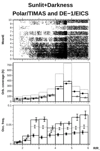
re-0 1 2 3 4 5 6 7 8 9 10 MeanE 0 100 200 300 400 500 600 700 Orb. coverage (h) 2 3 4 5 6 R/R_E 0 0.05 0.1 Occ. freq.

Polar/TIMAS and DE−1/EICS

Sunlit+Darkness

Fig. 3. Polar/TIMAS and DE-1/EICS ion beams in the nightside MLT sectors as a function of radial distance R. Top panel: Ion beam events (one event corresponds to 12 s sample) as a function of radial distance and peak energy. Middle panel: Hours spent by the instrument in each radial bin. Bottom panel: Occurrence frequency of ion beams (number of points in each bin divided by the number of samples coming from the bin). Small Kp(≤ 2) shown by filled

circles, large Kp(> 2) by triangles. Dotted line is both Kps put

together. All nightside MLT sectors (18–06) with both sunlit and darkness conditions are included. The ILAT range is 65–74.

ality not fully correlated. Thus, the error bars shown in this paper are most probably overestimates of the true error level. Although TIMAS and EICS agree within the error limits in the cases where they can be compared, the error limits are not very small in the intercomparison bins and thus there could, in principle, be underlying systematical differences between the two instruments that are masked by the statistical errors in the intercomparison bins that could become important later when one considers bins with smaller statistical errors. To see that this is not the case we note from Tables 1 and 2 that the differences between TIMAS and EICS are insignificantly small in nine cases out of ten, but in one case (MLT 22–

02, 4–4.5 RE radial bin), the occurrence frequencies differ

by 35%. A more detailed comparison shows that TIMAS in this bin disagrees not only with DE-1 in the same bin, but also with TIMAS (and DE-1) in the neighbouring bins (plots not shown). This suggests that the difference is due

to statistical fluctuations rather than a systematic error. We have also manually checked the TIMAS events contributing to this bin but did not find traces of nonphysical effects that could explain why TIMAS sees 500 data points containing an ion beam in 17 h, while it should see about 370 to make it agree with EICS.

We now discuss more quantitatively how the mutual dif-ference between EICS and TIMAS relates to their standard deviation error estimates. If E is the occurrence frequency measured with EICS and T is the corresponding quantity measured with TIMAS and 1E and 1T are their expected standard deviations (calculated based on the number of or-bital crossings as explained above), let us consider the quan-tity Q = |E − T |/(0.5 × (1E + 1T )), i.e. the ratio of the EICS-TIMAS discrepancy to the mean of their standard devi-ations. For the ten entries displayed in Tables 1 and 2, the Q values are, in ascending order, 0, 0.09, 0.09, 0.16, 0.26, 0.40, 0.56, 0.57, 0.62 and 1.7. All values of Q are thus smaller than unity, except one (1.7), which was discussed above in the previous paragraph. The interpretation of the Q values is such that, for example, Q = 0.09 means that the standard deviation (the quantity shown as error bars in all figures of this paper) is about 10 times larger than the actual discrep-ancy between the two instruments. The median Q value over the ten cases is 0.33. If this value is taken as representa-tive, it would mean that the error bars shown in this paper are overestimates by about a factor of three. This point should be kept in mind when looking at the figures, i.e. that the er-ror bars are probably unrealistically large. For the sake of keeping the plots mathematically rigorous we elected not to divide the error bars by 3 (or some other constant). In most cases the plotted error bars do not cause problems, i.e. we can draw our conclusions even with the displayed (overesti-mated) error bars.

We conclude that TIMAS and EICS data agree well enough so that when the ion beams are found and the er-ror bars are drawn in the manner described above, data from both satellites can be put in the same statistics.

3 Results

3.1 Radial distance

In Fig. 3 we show our baseline plot, which is TIMAS and EICS ion beams put together in the 0.5–10 keV energy range for all nightside MLT sectors under sunlit and darkness con-ditions. The occurrence frequency of ion beams generally increases with altitude, but there is also a relative maximum

in the occurrence frequency of ion beams at 3 RE radial

dis-tance. In the baseline case (dotted line in Fig. 3

represent-ing all Kps put together), the relative maximum (henceforth

called “the peak”) occurs at 2.75 REradial distance and a

lo-cal minimum at 3.75 RE. The existence of a peak can be seen

in earlier plots (Gorney et al., 1981; Yau et al., 1985; Kondo et al., 1990) but it has not been discussed.

3.2 Kp

Figure 3 shows small Kp(≤ 2) by filled circles and large Kp

(> 2) by triangles. The combined statistics are shown by a dotted line. Generally, the ion beam occurrence frequency

is ∼2–3 times larger for Kp > 2 than for Kp ≤ 2. The

peak and the minimum above it occur at 3.25 and 3.75 RE

for large Kp, respectively. For low Kp the peak also exists

but its amplitude is weak (of the order of the error bar).

3.3 MLT and solar illumination

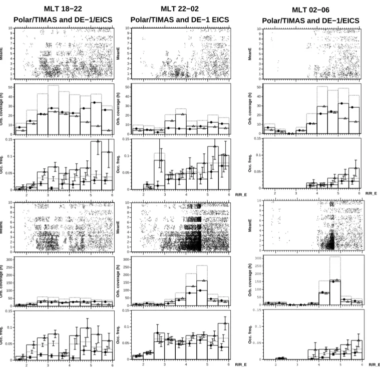
In Fig. 4 we show the ion beam statistics separated into three nightside MLT sectors in sunlit (top) and darkness (bottom)

conditions. Comparing radial distance bins below 2.5 REfor

high Kp conditions, the occurrence frequency in darkness

is 0.05, which is 2.5 times higher than in sunlit conditions in the evening sector (18–22 MLT). Overall, this is in agree-ment with a previous study where a ratio of ∼3 was found in the occurrence frequency in darkness versus sunlit beams (Collin et al., 1998), although the beam selection criteria and thus the absolute occurrence frequencies are different in the two studies. It is also seen that in the evening sector between

2.5 and 3.5 RE the occurrence rate of ion beams is higher

during darkness than during sunlit conditions, although the

difference is not as large as below 2.5 RE. In the midnight

(22–02) sector there is a pronounced peak at the 2.5–3 RE

bin in sunlit conditions, but its reliability is questionable due to the large error bars. In midnight darkness conditions the peak is less pronounced than in the evening sector, especially

for high Kp. High Kp midnight is the combination that is

most affected by substorms, so substorms are a likely can-didate for causing the difference between the midnight and the evening sectors in this respect. In a recent study of auro-ral cavities the midnight MLT sector was also found to have different behaviour which was attributed to substorms (Jan-hunen et al., 2002). In the morning sector ion beams are rare.

The relative peak in occurrence frequency around 3 RE

radial distance is most apparent in the evening sector (18– 22 MLT). In this sector we also have the best overall orbital coverage, so that the statistical errors are the smallest. In the morning sector there is no orbital coverage at all close to

3 RE so the existence of the peak remains uncertain in that

MLT sector.

Ion beams for small Kp are rare in other MLT sectors

ex-cept the midnight sector, where they are almost equally

com-mon for small and large Kp indices (except in the midnight

2.5–3 RE bin under sunlit conditions, which, however has

rather large error bars as we remarked above).

3.4 Solar cycle effects

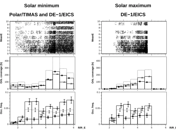
In Fig. 5 we show the statistics separated into solar mini-mum (left panel) and solar maximini-mum years (right panel). We take years 1978–1982, 1988–1992 and 1999–2003 to be solar maximum years. Other years are taken to be solar minimum. Thus, TIMAS (1996–1998) contributes to the solar minimum

statistics only. There is hardly any systematic dependence on the solar cycle. From the orbital coverage panels one sees

that during the solar maximum years, high Kp values are

always more common than small Kpvalues, while for solar

minimum years they are about equally common, which is not surprising.

3.5 ILAT dependence

To investigate ILAT dependence, we show in Fig. 6 the oc-currence frequency for all nightside MLT but decomposed into three ILAT ranges: 65–68 (bottom panel), 68–71

(mid-dle panel) and 71–74 (top panel). We see that small Kp

events occur only seldom below ILAT 68, which is natural. The occurrence frequency is largest in the 68–71 ILAT bin, which corresponds to the average auroral oval latitudes. For

high Kp, the peak is seen to exist at all ILAT ranges

sepa-rately.

Another view on the ILAT dependence is provided in Fig. 7, which shows the two-dimensional ILAT-altitude statistics of all nightside ion beams.

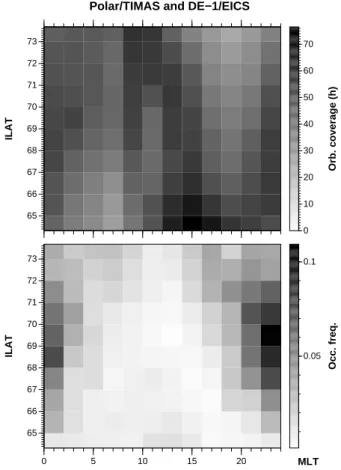
In Figs. 8 and 9 we show that statistics in the MLT-ILAT and MLT-R planes, respectively. In the MLT-ILAT plane the auroral dependence of ion beams is clearly seen, i.e. that beams occur at lowest ILAT close to midnight and that they occur most often near midnight, with a slight preference for pre-midnight. In Fig. 9 the auroral dependence can be seen

as well, together with the fact that the ∼3 REoccurrence

fre-quency peak is visible in essentially all MLT sectors (16–04) where there is orbital coverage and ion beams.

From Fig. 8 one sees that ion beams, when all altitudes are put together, occur mostly in the 22–24 MLT sector, in accor-dance with the results of Yau et al. (1985) and Gorney et al. (1985), whereas Johnson (1983) in his Fig. 5 found that ion beams, at least during disturbed conditions, occur mostly in the 15–21 MLT range. The results of Johnson (1983) repre-sent the altitude range 6000–8000 km only, however, which

corresponds to our second altitude bin (2–2.5 RE radial

dis-tance). Inspection of Fig. 4 shows that in this altitude bin,

ion beams for large Kp are indeed much more common in

the 18–22 than in the 22–02 MLT sector in our database. Thus, our results are also in agreement with those of

John-son (1983). Thus, at low altitude and high Kp, ion beams are

mainly an evening sector phenomenon, while at high altitude

and low Kpthey are more a midnight sector phenomenon.

3.6 Ion beam energy, particle flux and ion energies

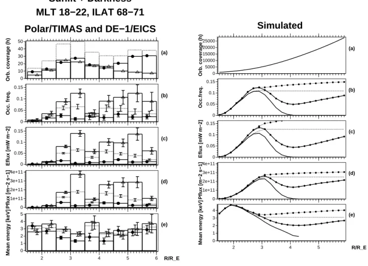
Thus far we have only considered the occurrence frequency of ion beams, but now we will study the energy and particle fluxes carried by the beams, as well as the mean energy for the evening sector. We limit ourselves to the evening sec-tor in this substudy, because in the morning secsec-tor we have only a few ion beams, as seen above, and in the midnight sector the situation is somewhat more complicated (see be-low). In Fig. 10, left panel, we show the invariant energy

0 1 2 3 4 5 6 7 8 9 10 MeanE 0 10 20 30 40 50 Orb. coverage (h) 2 3 4 5 6 0 0.05 0.1 0.15 Occ. freq.

Polar/TIMAS and DE−1/EICS MLT 18−22

Sunlit

Polar/TIMAS and DE−1 EICS MLT 22−02 0 1 2 3 4 5 6 7 8 9 10 MeanE 0 10 20 30 40 50 Orb. coverage (h) 2 3 4 5 6 R/R_E 0 0.05 0.1 0.15 Occ. freq.

Polar/TIMAS and DE−1/EICS MLT 02−06 0 1 2 3 4 5 6 7 8 9 10 MeanE 0 50 100 150 200 250 300 Orb. coverage (h) 2 3 4 5 6 0 0.05 0.1 0.15 Occ. freq.

Darkness

Fig. 4. Same as Fig. 3, but separated in the three nightside MLT sectors with sunlit (top) and darkness (bottom) conditions.

m−2s−1 carried by the upward ion beams (panel d). Both

quantities are altitude-invariant in the sense that they have been projected to the ionospheric plane by multiplying them by the magnetic field ratio. They have been averaged lin-early over all data points. Regions where no ion beams are detected are assumed to have zero energy and particle flux, thus, the quantities plotted tell how much energy and parti-cle flux is carried away from the ionosphere globally by ion beams, on average, in the 68–71 ILAT range and 18–22 MLT. If all ion beams could be reliably detected and if there were no wave-particle interactions, the conservation of beam par-ticles would dictate that the invariant particle flux should be

independent of altitude, if the external conditions (magnetic activity level, solar illumination condition, etc.) are also the same for all altitudes. From panel (d) of Fig. 10, left panel, we see that this is clearly not the case, as the invariant number flux generally varies with altitude. Thus, if we exclude in-strumental effects for a moment (they will be discussed later in this part and in the Discussion section below), it must be that beams in some altitude regions turn at least temporar-ily into something which is not recognizable as a beam any longer (e.g. ion conics). In other regions where the invariant particle flux increases with altitude it must happen that the conics turn back into beams (probably by the mirror force)

0 1 2 3 4 5 6 7 8 9 10 MeanE 0 100 200 300 400 Orb. coverage (h) 2 3 4 5 6 R/R_E 0 0.05 0.1 Occ. freq.

Polar/TIMAS and DE−1/EICS

Solar minimum

DE−1/EICS

Solar maximum

Fig. 5. Same as Fig. 3, but separated for solar minimum (left) and solar maximum years (right). All nightside MLT sectors with both sunlit and darkness conditions are included, and the ILAT range is 65–74.

or that new particles enter pre-existing beams or new beams are initiated at the altitude in question.

In Fig. 10, the invariant energy flux (panel c) and particle flux (panel d) altitude variation follow the variation of the oc-currence frequency of ion beams (panel b). If the only ener-gization mechanism were a potential drop acceleration below 8000 km, for instance, all three quantities should stay

con-stant above 8000 km (R = 2.25 RE). As seen from Fig. 10,

this is not the case, but all three quantities drop rather

dramat-ically at R = 3.75 RE for high Kp(for small Kp, the drop

occurs at 3.25). At higher altitudes they slowly recover. This suggests that some process operating at the altitude where the quantities drop is making the ion beams at least temporarily unrecognizable.

The last panel (panel e) of Fig. 10 is the mean beam energy (the mean invariant energy flux divided by the mean invariant particle flux). We will discuss this panel below, after present-ing a simple Monte Carlo simulation.

Here, we discussed only the evening sector. Similar trends in the invariant energy, particle fluxes, and ion mean energy

exist in the midnight sector for low Kp indices, but not for

high Kp. A probable reason for why the high Kpmidnight

sector behaves differently in this regard is that data in the

midnight sector during high Kp are probably dominated by

a direct influence of substorm phenomena.

3.7 Monte Carlo simulation of ion beams

A physical understanding of the altitude behavior of all the quantities shown in the left panel of Fig. 10 is not easy with-out some computer modelling. To this end we present a simple Monte Carlo simulation in which we generate 10000 ion beams. The invariant particle flux of each ion beam is a random number selected from the exponential distribution

(Press et al., 1992), with mean 5.44 × 1011m−2_s−1_{. The}

specific numerical constants have been selected to produce results that resemble those in the left panel of Fig. 10. The ion beam is assumed to have zero energy at the bottom of the acceleration region. The acceleration region is modelled by either an open or closed potential structure, whose depth is another exponentially distributed random number with

mean V0=2 kV. The potential structure V (R) is defined by

V (R) = V0exp(−((R−R0)/1R)2)in the closed case. Here,

Ris the radial distance in units of REand R0=(R1+R2)/2

and 1R = (R2−R1)/2 are parameters defining the center

de-0 0.05 0.1 Occ. freq. ILAT=71..74 ILAT=68..71 ILAT=65..68 0 0.05 0.1 Occ. freq. 2 3 4 5 6 R/R_E 0 0.05 0.1 Occ. freq.

Polar/TIMAS and DE−1/EICS

Sunlit + Darkness

Fig. 6. Same as the bottom panel of Fig. 3, but shown separately for the ILAT ranges 71–74 (top), 68–71 (middle) and 65–68 (bottom). All nightside MLT sectors (18–06) are put together, and both sunlit and darkness conditions are included.

pends on V0, so that R1 =max(2.5 − V0/5, 1.5) while R2

has the constant value 3.5. The parameters R1and R2

rep-resent the bottom and top altitudes of the potential structure, respectively, and their values have been selected to be physi-cally reasonable (Janhunen and Olsson, 2002). The open

po-tential structure case is obtained by setting V (R) to V0when

R > R0. The simulated ion beams are detected by many vir-tual instruments placed at different altitudes, using the same thresholds as are used when processing TIMAS and EICS data.

We now discuss an instrumental effect related to satellite speed. Due to the fast velocity at low altitude, the satel-lite traverses a rather long ILAT distance during one mea-surement cycle (12 s for Polar, 96 s for DE-1; we use 12 s in the simulation since the low-altitude data come from Po-lar). At the lowest altitude bin the north-south distance tra-versed during 12 s by Polar is about 24 km in the ionosphere, which is a longer distance than the width of narrow auroral arcs. Thus, the measured ion beams will be effectively aver-aged with background, which reduces their observed inten-sity (the particle and energy flux). However, the probability that the satellite hits an ion beam during 12 s is

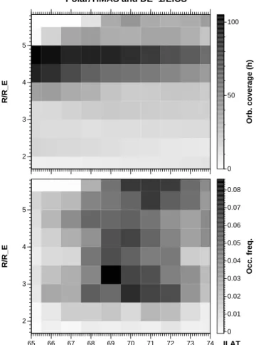
correspond-2 3 4 5 R/R_E Orb. coverage (h) 0 50 100 65 66 67 68 69 70 71 72 73 74 ILAT 2 3 4 5 R/R_E Occ. freq. 0 0.01 0.02 0.03 0.04 0.05 0.06 0.07 0.08

Polar/TIMAS and DE−1/EICS

Fig. 7. Top: Orbital coverage in hours in each bin. Bottom: Occur-rence frequency of all nightside 0.5–10 keV ion beams as a function of ILAT and radial distance R. Both TIMAS and EICS data are put together, as are all Kp values, all nightside MLT sectors (18–06),

and sunlit and darkness conditions.

ingly higher. Thus, there are two competing effects, the first decreasing and the second increasing the probability of de-tecting ion beams at low altitude. Since the first effect is ex-ponential and the second one is only linear, the net effect is a reduction of the probability of detecting beams. We model both of these satellite speed related effects by using a realistic satellite velocity altitude dependence profile.

In the simulation we assume that the average width of ion beams’ regions when mapped to the ionosphere is 8 km. The widths of the ion beams should match the typical widths of inverted-V regions and optical auroral arcs. The widths of inverted-V regions and optical arcs match each other when compared with compatible criteria (Stenbaek-Nielsen et al., 1998). The widths of optical arcs vary, but 8 km is a typical value.

Optionally, uniform wave energization (constant energy increment in each altitude step) is added into the simula-tion. The wave energization W (R) is taken to be

propor-tional to V0and taken to start from R = 2, so that W (R) =

0.2eV0max(R − 2, 0). When wave energization is on, the

65 66 67 68 69 70 71 72 73 ILAT Orb. coverage (h) 0 10 20 30 40 50 60 70 0 5 10 15 20 MLT 65 66 67 68 69 70 71 72 73 ILAT Occ. freq. 0.05 0.1

Polar/TIMAS and DE−1/EICS

Fig. 8. Top: Orbital coverage in hours in each bin. Bottom: Occur-rence frequency of all 0.5–10 keV ion beams as a function of MLT and ILAT for all radial distances smaller than 6 RE. All Kpvalues,

all radial bins and data from both TIMAS and EICS are put together. The dayside MLT range 10–14 may contain data errors and should not be looked at.

otherwise, from E = eV (R). The invariant energy flux is simply the invariant particle flux multiplied by E.

The right panel of Fig. 10 shows four cases: closed poten-tial without wave energization (solid line), closed potenpoten-tial with wave energization (solid line with black circles), open potential without waves (dotted line), and open potential with waves (dotted line with black circles). We see that the model with a closed potential and wave energization corresponds to the left panel of Fig. 10 quite well, while the other models have severe problems in reproducing some of the features in the data.

Intuitively, one could expect that the mean energy of ions should increase when the ions move inside a potential struc-ture and are speeded up. Looking at Fig. 10 (panel e), this is not the case, however, but rather there is a decrease. The main reasons are the satellite speed dependent effects

dis-cussed above. The reason why there is a slight peak at

R = 2 RE in the mean energy (Fig. 10, panel e), even in

the U-potential curves (dotted lines), is that at R < 2RE

part of the potential drop is still above the satellite, so the

mean energy is smaller for that reason and at R = 2 RE,

only the strongest beams are detectable due to the satellite

2 3 4 5 R/R_E Orb. coverage (h) 0 50 100 150 0 5 10 15 20 MLT 2 3 4 5 R/R_E Occ. freq. 0 0.01 0.02 0.03 0.04 0.05 0.06 0.07 0.08

Polar/TIMAS and DE−1/EICS

Fig. 9. Top: Orbital coverage in hours in each bin. Bottom: Occur-rence frequency of all 0.5–10 keV ion beams as a function of MLT and radial distance R for all ILAT in the range 65...74. Both TIMAS and EICS data are put together, as are all Kpvalues, with sunlit and

darkness conditions. The dayside MLT range 10–14 may contain data errors and should not be looked at.

speed smearing-out effect and thus, the high energy beams are overrepresented.

We verified that the results do not change much if the de-tails of the potential structure bottom altitude dependence are changed or replaced by random numbers. To achieve realis-tic results it is only of importance that some variations of the potential structure bottom altitude occur. Such variations can be caused by the seasonal dependence, for example.

4 Discussion

In this study we have confirmed previous results, such as the fact that ion beams occur less often in the morning sector than in the evening and midnight sectors and that low altitude

beams (< 2.5 RE) occur more often when the ionosphere is

in darkness than when it is illuminated by the Sun. Also, the result that ion beam occurrence frequency increases with

increasing Kpindex is in accordance with previous studies.

The most interesting result is that there is a peak in

occur-rence frequency at ∼3 REradial distance. (Equivalently, one

0 10 20 30 40 50 Orb. coverage (h) 0 0.05 0.1 0.15 Occ. freq. 0 0.05 0.1 0.15 Eflux [mW m−2] 0 1e+11 2e+11 3e+11 4e+11 Pflux [m−2 s−1] 2 3 4 5 6 R/R_E 0 1 2 3 4 5

Mean energy [keV]

Polar/TIMAS and DE−1/EICS

MLT 18−22, ILAT 68−71

Sunlit + Darkness

Mean energy [keV]

Simulated

Fig. 10. Left panel: Mean energy and particle fluxes carried by ion beams in the evening MLT sector (18–22) and ILAT range 68–71. (a) Orbital coverage in hours, (b) occurrence frequency of ion beams, (c) average invariant energy flux (“invariant” means the quantity is projected to ionospheric altitude), (d) average invariant particle flux, (e) mean energy (panel c divided by panel d). Right panel: Four simulated examples (see text), solid line corresponds to a closed potential structure and dotted line to an open structure; lines with black circles correspond to cases having additional wave energization (see text).

3.75 RE.) The peak can also be seen as an enhancement in

invariant energy and particle fluxes. A peak in occurrence frequency can be seen in earlier plots (Yau et al., 1984, Fig. 4, right panel; Kondo, 1990, Fig. 7 right panel; Peterson et al., 1992, Fig. 2, top left panel), but it has not been investigated more closely. These earlier studies use DE-1 data, which, in our case, is the only contributor at the peak altitude, so the earlier results are in this sense not independent from ours, al-though our use of Polar data in this study has allowed us to validate DE-1 data at low and high altitude. Another result is

an increase in ion beam occurrence frequency for R > 4 RE;

it is not possible to obtain this result with DE-1 alone because

DE-1 apogee radial distance is 4.5 RE. We will now itemize

our main results:

1. In the baseline case (all MLT, ILAT, Kp and solar

il-luminations conditions put together), a peak in

occur-rence frequency of ion beams exists at 2.75 RE radial

distance, and a local minimum occurrence frequency

above it at 3.75 RE.

2. When considering low and high Kpseparately, the solar

cycle does not have a notable influence on the ion beam occurrence frequency.

3. In the evening sector, a peak is also present in the in-variant energy and particle fluxes carried by upward ion beams, where “invariant” means that both quantities are projected to the ionospheric plane. In the midnight

sec-tor (plots not shown) there is a peak for low Kp, but not

for high Kp; the high Kpstatistics in the midnight

sec-tor is probably dominated by a direct influence of sub-storms, which makes the situation more complicated. 4. The peak appears in all ILAT ranges, but is most visible

in the 68–71 ILAT bin, probably because it corresponds to the average auroral oval latitude.

5. At low altitude (R < 2.5 RE) and high Kp, ion beams

altitude (R > 3 RE, say) and low Kp they are more a midnight sector phenomenon. The reasons remain un-known, but need further investigation. The result sug-gests that ion beams in the midnight sector do not

di-rectly come from the region 2.5 RE, rather they are the

result of processes acting at intermediate altitudes. 6. Our simple Monte Carlo simulation demonstrates that a

closed potential structure with some wave energization can explain the altitude dependence of the ion beam oc-currence frequency, energy flux, particle flux and mean energy in the evening sector (Fig. 10).

Since the ∼ 3 REpeak (or, equivalently, the dip above it)

is the main result of the paper, it is appropriate to try to also list the possible instrumental explanations for it. We now discuss three such instrumental explanation attempts for the peak seen in the occurrence frequency of ion beams and rule them out one by one:

1. The flux tube scaling dictates that the number flux of an

ion beam with ionospheric origin will decay as R−3.

This implies that weak beams fall below the

instru-ment threshold from some altitude upwards.

How-ever, the mapped-to-ionosphere instrument threshold for both Polar/TIMAS and DE-1/EICS is about ten

times smaller, even at the highest altitude (6 RE) and

highest energy (10 keV) than our imposed invariant

en-ergy flux threshold of 0.2 mW m−2_{, so the flux tube}

scaling effect does not play any role in our study. We also checked with the Monte Carlo simulation that, al-though the flux tube scaling effect can, if one assumes unrealistic instrument threshold values, produce a peak and a subsequent smooth depression, it can never pro-duce the observed subsequent increase at higher alti-tudes.

2. The peak does not disappear when the data are studied separately for different geomagnetic disturbance levels

(Kp index), solar cycle phase, solar illumination

con-dition, magnetic local time and invariant latitude. This rules out the possibility that the peak could be due to a correlated time/altitude orbital characteristic, together with some instrumental problem that persisted in a cer-tain time period.

3. As pointed out in more detail in Sect. 3.7 above, satellite speed related effects decrease the probability of seeing ion beams at low altitude. This effect does not, however, explain the existence of the peak.

We will now discuss possible physical mechanisms re-sponsible for the peak in the occurrence frequency of ion beams and thereafter, the high-altitude ion beam behavior.

The possibility for a downward field in the 15 000– 20 000 km altitude range has been invoked as one of the pos-sibilities when trying to understand counterstreaming ions (Sagawa et al., 1987; Horita et al., 1987). Later, a

down-ward electric field in the 3–4 RE radial range has also been

proposed as an explanation for the lack of auroral potential

structures above 4 RE radial distance (Janhunen et al., 1999;

Janhunen and Olsson, 2000). Our Monte Carlo simulations demonstrated (Sect. 3.7 above) that indeed, a closed potential structure is able to explain the occurrence frequency peak of the ion beams.

Beam ions are likely to be energized by both auroral po-tential structures and waves. This is already evident from the fact that one often sees ion beams of 10–20 keV energy in TIMAS data (even energies as high as 40 keV have been reported, Lundin and Eliasson, 1991), while potential struc-tures of comparable magnitude are rare (Olsson et al., 1998). Also, the fact that the ion beam occurrence frequency

con-tinues to increase at high altitudes (R > 4 RE) suggests that

there is continuous wave-induced ion heating or parallel elec-tric fields at high altitude.

Indeed, to explain the increase in the ion beam occurrence frequency at high altitude quantitatively, some wave ener-gization was necessary to insert in the Monte Carlo simula-tion of Sect. 3.7. Other explanasimula-tions (in particular, those that involve an open potential structure or no significant potential structure at all) might perhaps be constructed, but they should by necessity include rather strongly altitude-dependent wave heating or some other altitude-dependent process not in-cluded in our model.

Even when the wave amplitudes are altitude-independent, the efficiency of perpendicular wave heating should be in-versely proportional to the ion beam velocity, because the wave heating per unit altitude interval is proportional to the time the particles spend within the interval. Coming back to the Monte Carlo model, the ion beams, therefore, slow down where there is downward electric field and thus, the perpendicular heating (energization) should be locally en-hanced. The result could be that some of the beams turn into

ion conics. Ion conics are indeed observed at ∼ 3 REradial

distance (Klumpar et al., 1984), where the slowing down of the beam occurs in our model. At higher altitude the mirror force would turn them into beams again as the energy ob-tained from the waves would be gradually turned from per-pendicular to parallel kinetic energy. An analogous process operating in the return current region below 7000 km altitude has been discussed earlier by Gorney et al. (1985) and has recently been confirmed by FAST observations (Ergun et al., 1998). This additional effect was not included in the Monte Carlo simulation, but if included, it could make the dip above the occurrence frequency peak stronger than what the simula-tion produced, thus perhaps further increasing the agreement with data (Fig. 10, left panel).

Upward parallel electric fields at high (R > 4 RE)

alti-tude could, in principle, also be a possibility to explain ion beam energization at that altitude range, but this explanation is rather unlikely as we are not aware of inverted-V electron signatures at that altitude, at least not with keV energies. If such a structure would exist, it should occur in combination with a closed potential structure at lower altitude, in order to explain the peak.

More statistical studies of the altitude dependence of pa-rameters other than ion beams (auroral potential structures,

density cavities (Janhunen et al., 2002), waves, and electron anisotropies) are completed or in progress by us and may help resolve the question of the potential structures and their associated wave-particle interactions more fully.

No matter what the processes are that explain the peculiar

behavior at ∼ 3 RE radial distance, it is clear that there is a

nontrivial and relatively narrow altitude range around 3–4 RE

radial distance that seems thus far to have received too little attention in auroral physics.

Acknowledgements. Acknowledgements. The work of AO is sup-ported by the Swedish Research Council and that of PJ by the Academy of Finland. TIMAS data were produced under support of NASA contract NAG-53032 to Lockheed Martin and NAG5-11391 to the University of Colorado. We are grateful to NASA for making TIMAS data available through CDAWeb.

The Editor in Chief thanks E. Sagaura and another referee for their help in evaluating this paper.

References

Andr´e, M. and Yau, A.: Theories and observations of ion energiza-tion and outflow in the high latitude magnetosphere, Space Sci. Rev., 80, 27–48, 1997.

Collin, H. L., Peterson, W. K., Lennartsson, O. W., and Drake, J. F.: The seasonal variation of auroral ion beams, Geophys. Res. Lett., 25, 4071–4074, 1998.

Ergun, R. E., Carlson, C. W., McFadden, J. P., et al.: FAST satel-lite observations of electric field structures in the auroral zone, Geophys. Res. Lett., 25, 2025–2028, 1998.

Frank, L. A. and Ackerson, K. L.: Observations of charged particle precipitation into the auroral zone, J. Geophys. Res., 76, 3612– 3643, 1971.

Gorney, D. J., Clarke, A., Croley, D., Fennell, J., Luhmann, J., and Mizera, P.: The distribution of ion beams and conics below 8000 km, J. Geophys. Res., 86, 83–89, 1981.

Gorney, D. J., Chiu, Y. T., and Croley, Jr., D. R.: Trapping of ion conics by downward parallel electric fields, J. Geophys. Res., 90, 4205–4210, 1985.

Hallinan, T. J. and Stenbaek-Nielsen, H. C.: The connection be-tween auroral acceleration and auroral morphology, Phys. Chem. Earth, 1–3, 26, 169–177, 2001.

Horita, R. E., Ungstrup, E., Shelley, E. G., Anderson, R. R., and Fitzenreiter, R. J.: Counterstreaming ion events in the magneto-sphere, J. Geophys. Res., 92, 13 523–13 536, 1987.

Janhunen, P., Olsson, A., Mozer, F. S., and Laakso, H.: How does the U-shaped potential close above the acceleration region? A study using Polar data, Ann. Geophysicae, 17, 1276–1283, 1999. Janhunen, P. and Olsson, A.: New model for auroral acceleration: O-shaped potential structure cooperating with waves, Ann. Geo-physicae, 18, 596–607, 2000.

Janhunen, P., Olsson, A., Peterson, W. K., Laakso, H., Pickett, J. S., Pulkkinen, T. I., and Russell, C. T.: A study of inverted-V auro-ral acceleration mechanisms using Polar/Fast Auroauro-ral Snapshot conjunctions, J. Geophys. Res., 106, 18 995–19 011, 2001. Janhunen, P. and Olsson, A.: A hybrid simulation model for a stable

auroral arc, Ann. Geophysicae, 20, 1–14, 2002.

Janhunen, P., Olsson, A., and Laakso, H.: Altitude dependence of plasma density in the auroral zone, Ann. Geophysicae, 20, 1743– 1750, 2002.

Janhunen, P., Olsson, A., Vaivads, A., and Peterson, W. K.: Gener-ation of Bernstein waves by ion shell distributions in the auroral region, Ann. Geophysicae, 21, 881–891, 2003.

Johnson, R. G.: That hot ion composition, energy, and pitch an-gle characteristics above the auroral zone ionosphere, in: High-latitude space plasma physics, edited by Hultqvist, B. and Hag-fors, T., Plenum, New York, pp. 271–294, 1983.

Klumpar, D. M., Peterson, W. K., and Shelley, E. G.: Direct evi-dence for two-stage (bimodal) acceleration of ionospheric ions, J. Geophys. Res., 89, 10 779–10 787., 1984.

Kondo, T., Whalen, B. A., and Yau, A. W.: Statistical analysis of upflowing ion beam and conic distributions at DE 1 altitudes, J. Geophys. Res., 95, 12 091–12 102, 1990.

Lin, C. S. and Hoffman, R. A.: Characteristics of the inverted-V event, J. Geophys. Res., 84, 1514–1525, 1979.

Lundin, R. and Eliasson, L.: Auroral energization processes, Ann. Geophysicae, 9, 202–223, 1991.

McFadden, J. P., Carlson, C. W., Ergun, R. E. et al.: Spatial structure and gradients of ion beams observed by FAST, Geophys. Res. Lett., 25, 2021–2024, 1998.

Miyake, W., Mukai, T., and Kaya, N.: On the origins of the up-ward shift of elevated (bimodal) ion conics in velocity space, J. Geophys. Res., 101, 26 961–26 969, 1996.

M¨obius, E., Tang, L., Kistler, L. M., et al.: Species dependent ener-gies in upward directed ion beams over auroral arcs as observed with FAST TEAMS, Geophys. Res. Lett., 25, 2029–2032, 1998. Olsson, A., Andersson, L., Eriksson, A. I., Clemmons, J., Erlands-son, R. E., Reeves, G., Hughes, T., and Murphree, J. S.: Freja studies of the current-voltage relation in substorm related events, J. Geophys. Res., 103 4285–4301, 1998.

Peterson, W. K., Collin, H. L., Doherty, M. F., and Bjorklund, C. M.: O+and He+restricted and extended (bi-modal) ion conic ditributions Geophys. Res. Lett., 19, 1439–1442, 1992. Press, W. H., Teukolsky, S. A., Vetterling, W. T., and Flannery, B.

P.: Numerical Recipes in C, The art of scientific computing, 2nd ed., Cambridge, 1992.

Sagawa, E., Yau, A. W., Whalen, B. A., and Peterson, W. K.: Pitch angle distributions of low-energy ions in the near-earth magneto-sphere, J. Geophys. Res., 92, 12 241–12 254, 1987.

Shelley, E. G., Simpson, D. A., Saunders, T. C., Hertzberg, E., Bal-siger, H., and Ghielmetti, A. G.: The energetic ion composition spectrometer (EICS) for the Dynamics Explorer-A, Space Sci. Instrum., 5, 443, 1981.

Shelley, E. G., Ghielmetti, A. G., Balsiger, H., Black,R. K., Bowles, J. A., Bowman, R. P., Bratschi, O., Burch, J. L., Carlson, C. W., Coker, A. J., Drake, J. F., Fischer, J., Geiss, J., Johnstone, A., Kloza, D. L., Lennartsson, O. W., Magoncelli, A. L., Paschmann, G., Peterson, W. K., Rosenbauer, H., Sanders, T. C., Steinacher, M., Walton, D. M., Whalen, B. A., and Young, D. T.: The Toroidal Imaging Mass-Angle Spectrograph (TIMAS) for the Polar Mission, Space Science Rev., 71, 1–4, 1995.

Stenbaek-Nielsen, H. C., Hallinan, T. J., Osborne, D. L., Kimball, J., Chaston, C., McFadden, J., Delory, G., Temerin, M., and Carl-son, C. W.: Aircraft observations conjugate to FAST: auroral arc thickness, Geophys. Res. Lett., 25, 2073–2076, 1998.

Yau, A. W., Whalen, B. A., Peterson, W. K., and Shelley, E. G.: Distribution of upflowing ionospheric ions in the high-altitude polar cap and auroral ionosphere, J. Geophys. Res., 89, 5507– 5522, 1984.

Yau, A. W., Shelley, E. G., Peterson, W. K., and Lenchyshyn, L.: Energetic auroral and polar ion outflow at DE 1 altitudes: magni-tude, composition, magnetic activity dependence, and long-term variations, J. Geophys. Res., 90, 8417–8432, 1985.