Direct numerical simulations of multiphase flow with applications to basaltic volcanism and planetary evolution

Direct numerical simulations of multiphase flow

with applications to basaltic volcanism and

planetary evolution

by

Jenny Suckale

M.P.A., Harvard Kennedy School, 2006

Diploma, Free University of Berlin, 2002

MASSACHUSETTS INSTITUTE

OF TECHNOLOY~

OCT

2 5 2011

LARARIES

ARCHIVES

Submitted to the Department of Earth, Atmospheric, and Planetary

Sciences

in partial fulfillment of the requirements for the degree of

Doctor of Philosophy

at the

MASSACHUSETTS INSTITUTE OF TECHNOLOGY

June 2011

®

Massachusetts Institute of Technology 2011. All rights reserved.

A u th or ...

...

Department of Earth, Am

eri

nd Planetary Sciences

ID/)

May

4, 2011

Certified by...

Linda T. Elkins-Tanton

Mitsui Career Development Assistant Professor of Geology

Thesis Supervisor

Accepted by.../

Maria Zuber

E. A. Griswold Professor of Geophysics

Direct numerical simulations of multiphase flow with

applications to basaltic volcanism and planetary evolution

by

Jenny Suckale

Submitted to the Department of Earth, Atmospheric, and Planetary Sciences on May 4, 2011, in partial fulfillment of the

requirements for the degree of Doctor of Philosophy

Abstract

Multiphase flows are an essential component of natural systems: They affect the explosivity of volcanic eruptions, shape the landscape of terrestrial planets, and govern subsurface flow in hydrocarbon reservoirs. Advancing our fundamental understanding and predictive capabilities of multiphase flows is a problem of immense importance for both industrial and scientific purposes.

This thesis studies the potential of direct numerical simulations for advancing our fundamental understanding of the multiphase flow dynamics in magmatic flow. It is divided into two parts. The first part investigates gas-fluid coupling during the buoyant ascent of an exsolved gas phase in the conduit of basaltic volcanoes. The second part examines the solidification processes in magma oceans which entail both degassing (gas-fluid coupling) and crystallization (solid-fluid coupling).

For both applications, we find that the fluid dynamics at the length scale of the interfaces has important ramifications for the large-scale behavior of the system. We conclude that direct numerical simulations are an interesting complement to more tra-ditional computational approaches and may provide new insights into the complexity of magmatic systems.

Thesis Supervisor: Linda T. Elkins-Tanton

Acknowledgments

First and foremost, I would like to express my heartfelt gratitude to my advisor Lindy Elkins-Tanton. She is one of the most dedicated and hard-working people I have ever met and throughout my time at MIT, she has been a constant source of energy, ideas, and enthusiasm. It has been a privilege working with her and she will be an inspiration to me for years to come, both as an exceptionally productive scientist and as an uniquely supportive advisor.

I am also deeply indebted to Brad Hager for sparking my interest in

geodynam-ics and for countless stimulating and thought-provoking discussions. My meetings with Brad have been a much needed constant throughout my PhD and his brilliant perspectives on my work have profoundly shaped my thinking and my thesis.

This thesis would not have been possible without the continued support and in-valuable input from James Sethian at UC Berkeley. He has been a seemingly bottom-less source of numerical wisedom, an encouraging mentor, and a wonderful collabora-tor. My frequent and extended stays at the Lawrence Berkeley National Laboratory

(LBNL) have opened up a whole new world of numerical possibilities for me and have

transformed my thinking about the capabilities of modern computation for advancing Earth science. The exceptional hospitality of the applied math group at LBNL has also made these trips not only an intellectual adventure but a personal treat. I would like to thank the entire group for a warm welcome and Jiun-der Yu, Chris Rycroft, Marcus Roper, Per Olof Persson, Grigory Barenblatt, and Alexandre Chorin for in-sightful discussions. While at Berkeley, I also greatly enjoyed my visits to Michael Manga and his research group.

I am truly grateful to Kathy Cashman at the University of Oregon for her abso-lutely irresistible enthusiasm for volcanology in general and Stromboli in particular. Her invite to visit her and her research group in Oregon sparked an enjoyable and productive collaboration that I hope will carry well into the future. The frequent discussions with Kathy and her graduate student Isolde Belien about the field data for Stromboli have provided an essential counter-balance to my more theoretical

in-clinations and a fantastic learning opportunity.

The high-powered research environment at EAPS has been a wonderful potential to tap into. In particular, I would like to thank Stephane Rondenay for giving me the opportunity to explore field work in Greece and Maria Zuber and Ben Weiss for being on my thesis committee and providing helpful feedback. I also greatly benefited from discussions with Wiki Royden, Brian Evans, Tim Grove, Mike Fehler, Rob van der Hilst and Alison Malcolm.

MIT seems to be one of the few institutions that is more than the sum of its parts, which makes it easy to reach across disciplines. In particular, I would like to acknowledge the numerous inspiring exchanges about numerics (and free espressos) with Jean-Christophe Nave, now at McGill University, with whom I took my first numerics class at MIT and who then became an important collaborator. I also greatly enjoyed the discussions with Benjamin Seibold, John Bush, and Ruben Rosales at the Department of Mathematics.

When I started my PhD, many friends warned me that it would be a lonely endeavour. I could not say that I found that to be true. I think it takes a village to produce a PhD. The students at EAPS are the foundation of the department and it has been wonderful to be part of that vibrant community. The stimulating discussions I had with my fellow students over the years are countless and could not possibly be listed here, but I do want to briefly mention my various office mates of the years, Lindy's research group and the fun group meetings, and Einat Lev, Chin-Wu Chen, Mike Krawczynski, Alexandra Hosa, Yang Zhang, Andrea Llenos, and many others. I would also like to thank Linda Meinke and Scott Blomquist, who frequently went out of their way to solve a computer crisis; Brenda Carbone, Kerin Willis, and Terri Macloon for their kindness and administrative assistance; Roberta Allard for her invaluable support with scheduling challenges; and Vicki McKenna and Carol Sprague for always being there when I needed their help with organization difficulties and for always finding a solution. Last but certainly not least, I want to acknowledge Joe Hankins and Chris Sherratt from MIT libraries whose close to magical skills in finding absolutely irretrievable articles I deeply admire.

My loving parents, Gude Suckale-Redlefsen and Robert Suckale, have instilled in

me the deep appreciation for the pursuit of new knowledge that has carried me through my PhD. The persistent curiosity of and lively discussions with my in-laws, Bernd and Hiltrud Hainmueller, frequently reminded me of why I ever wanted to do a PhD. My brother, Jakob, has been a steady companion through both personal and scientific ups and downs and sharing this experience with him means the world to me. His fiancee, Ana Garcia-Saez, has brought more sunshine into my family that we all bask in, hopefully for many years to come. Anke Conway-Moritz and her men provided continued and essential moral support. Mortiz Hainmueller and Julia Piischel were among the few who ever made it to Boston for a much enjoyed and enjoyably science-free visit. Thy Nowak-Tran and young master Thao have provoked countless laughs and smiles when little else could and the numerous phone conversations with my girls in Berlin allowed me to travel back home whenever I needed to. The lunches with Ona Ferguson were always a welcome break and the christmases and dinner parties with Sebastian Bauhoff and Eliana Carranza true highlights.

Finally, very special thanks go to the love of my life and husband, Jens Hain-mueller, who always finds a way to believe in me even if I no longer do. His unwaver-ing encouragement for pursuunwaver-ing my dreams, his infallible intuition for knowunwaver-ing when I really needed a skiing or hiking break, his otherworldly patience for my mood swings,

and his scientific curiosity for both his field and mine will never cease to amaze me. He is the center of my life and the source of my greatest happiness.

Contents

1 Introduction 37

2 Modeling rapidly deforming interfaces in buoyancy-driven flow with

large viscosity contrasts 43

2.1 Introduction . . . . 43

2.2 Governing equations.. . . . . . . . 46

2.3 Numerical method . . . . 49

2.3.1 Ghost-fluid-type fluid solver . . . . 49

2.3.2 Level-set-based Interface solver . . . . 54

2.3.3 Coupling of the two solvers . . . . 56

2.4 Benchmark problems . . . . 57

2.4.1 Pressure jump at the interface of a viscous drop . . . . 57

2.4.2 Pressure jump for weak inclusions in pure shear . . . . 58

2.4.3 Rayleigh-Taylor instability . . . . 59

2.4.4 Compositional plume . . . . 60

2.5 R esults . . . . 61

2.5.1 Pressure jump at the interface of a viscous drop . . . . 61

2.5.2 Pressure jump for weak inclusions in pure shear . . . . 62

2.5.3 Rayleigh-Taylor instability . . . . 65

2.5.4 Compositional plume . . . . 65

2.6 D iscussion . . . . 66

2.6.1 Evaluation of the fluid solver . . . . 66

2.6.3 Coupling of the solvers . . . .

2.7 Conclusion ... . . . .

3 Bubble dynamics in basaltic volcanoes and ramifications for

model-ing normal Strombolian activity

Introduction . . . .. Governing equations and scaling analysis . . . . Theoretical estimates of bubble breakup . . . .

Sim ulations . . . . 3.4.1 Modeling approach . . . .

3.4.2 Stability analysis of isolated gas bubbles . . . .

3.4.3 Impact of multibubble interactions on stability dynam ics . . . .

3.4.4 Stability analysis of conduit-filling gas pockets .

3.5 Results . . . .

and interface

. . . . . . . . 89

. . . . . 90

. . . . 91

3.5.1 Dynamic instability of isolated gas bubbles during ascent . . . 91

3.5.2 Effect of multibubble interactions on breakup. . . . .. 95

3.5.3 Dynamic instability of slugs . . . . 99

3.6 D iscussion . . . . 101

3.6.1 Comparison of theoretical and numerical constraints on bubble breakup . . . . 101

3.6.2 Non-dimensional conditions for a coalescence cascade . . . . . 103

3.6.3 Non-dimensional conditions for stable slug rise . . . . 106

3.7 C onclusions . . . . 108

4 Slug or plug? A new look at the mechanism of normal activity at

Stromboli

111

4.2 Plug model of normal Strombolian activity... . . . . . . . . .. 115

4.3 R esults . . . . 117

4.3.1 Failure of the plug . . . . 117 3.1

3.2

3.3

3.4

4.3.2 Mechanism of normal eruptions. . . . .. 119 4.3.3 Conclusion . . . . 122

5 The possibility of catastrophic magma ocean degassing and

implica-tions for the formation of early planetary atmospheres

5.1 Introduction . . . .

5.2 M odel . . . .

5.2.1 Bubble dynamics at microscopic scales .

5.2.2 Degassing at macroscopic scales . . . . .

5.3 R esults . . . .

5.3.1 Early phase of magma ocean solidification

5.3.2 Late phase of magma ocean solidification 5.4 D iscussion . . . .

5.4.1 Catastrophic degassing of magma oceans 5.4.2 Water hitching its way up to the surface 5.4.3 Extent of early melting might determine t 5.4.4 Three end-member cases of degassing . .

5.5 Conclusion . . . .

[he fate of volatiles

125

6 Direct numerical simulations of solid-fluid

suspensions

r momenta

6.4.2 Flow over a square cylinder . . . .

coupling in crystalline

153

6.4.3 Sedimentation of a single sphere . . . . 172

6.4.4 Sedimentation of two interacting spheres . . . . 174

6.5 C onclusion . . . . 176

7 When crystals collide: Constraints on the fate of terrestrial planets

during magma ocean solidification

177

7.2 M odel . . . . 180

7.3 R esults . . . . 185

7.3.1 Very dilute suspensions . . . . 186

7.3.2 Dilute suspensions of equisized crystals . . . . 188

7.3.3 Dilute suspensions with heterogeneous crystal-size distributions 194 7.4 D iscussion . . . . 199

7.4.1 Vesta: Skewed crystal-size distributions may facilitate early crystal settling . . . . 199

7.4.2 The Moon: The possibility of crystal settling during the late stages of solidification . . . . 202

7.4.3 Conclusions . . . . 208

A Supplement for chapter 2

211

A.2 Pressure jump for weak inclusions at extremely large viscosity contrasts 214 A.3 Convergence tests for benchmark problems 1, 2, and 3 . . . . 214

A.4 Possible biases related to iterative reinitialization techniques . . . . . 218

A.5 Subgrid features . . . . 220

B Supplement for chapter 3

223

B.2 Dependence of breakup time on bubble radii for large bubbles . . . . 225

B.3 Resolution restriction for breakup induced by multibubble interactions 225 B.4 Convergence tests.. . . . . . . . 227

C

Supplement for chapter 4

231

C.1 Bubble and crystal populations in HP magma . . . . 231 C.2 Analytic solution for the stresses in an elliptic plate of moderate

thick-ness with clamped edges . . . . 233 C.3 Numerical approach for plugs with large thicknesses . . . . .. 236

C.4 Stress concentration at the microscopic scale . . . . 236

D Supplement for chapter 5

239

D.1 Homogeneous nucleation . . . . 239

E Supplement for chapter 6

241

List of Figures

2-1 Comparison of the standard (top) and ghost fluid (bottom) construc-tion of finite-difference stencils for computing the pressure gradient in the vicinity of the interface. The interface between fluid 1 and 2 is located between grid points (i,

j)

j).

of the interface is not taken into account (top), the finite-difference

approximation of the derivative

DP/ax

be

0(1)

into the domain of the other yielding two 'ghost' phases (bottom). After this extension, two values for pressure are associated with grid point (i + 1,j), the physical pi+1,j and the ghost value p+1,j. The ghost phases fulfill the additional purpose of enforcing the jump con-ditions at the interface. The jump concon-ditions

[P)

computed on both sides of the interface and then interpolated to re-flect the subgrid position of the interface. This yields the jump at the interface denoted as

[P]r,j.

2-2 Illustration of the construction of the asymmetric finite-difference sten-cil for the second derivative of the velocity field in one dimension. Two neighboring grid cells of size Ax are shown. The two fluids are shaded in grey and white, respectively, implying that the interface crosses only the grid cell on the right. The symmetric three-point stencil com-monly used to compute the second derivative of the velocity at point

ui, is indicated by crosses. In order to take the subgrid position of

the interface explicitly into account, we shift the central point in the symmetric stencil uij to coincide with the interface uIj. This leads to an asymmetric stencil indicated by black dots and spanned by the points ui_1,, urj and ui+1,j. - . - - - . - - . - - . - - . . . . 47

2-3 Initial and boundary conditions for the Rayleigh-Taylor instability as specified by [296]. The fluids are characterized by different densities pi and viscosities p. The level set function is constructed such that it is negative within the buoyant fluid and positive outside. . . . . 56 2-4 Computation of the pressure jump inside a static drop as a consequence

of surface tension (benchmark problem 1). The Bond number (eq. 2.10) is set to rI3 = 10-3 to ensure sphericity of the drop. The viscosity

contrast is 1 = 10-6. The point-wise visualization of the pressure

field illustrates the original resolution of the simulation (51 x 51). The computational domain is a square box of aspect ratio 1. . . . . 58

2-5 Computation of the pressure field associated with a dynamic drop ris-ing under its own buoyancy. The Bond number (eq. 2.10) is set to IH3 = 10-3 to ensure sphericity of the drop. The point-wise

visual-ization of the pressure field highlights the original resolution of the simulation (81 x 121). The computational domain is a rectangular box of aspect ratio 2 x 3. The pressure field is a combination of the discontinuous jump at the interface and the hydrostatic and dynamic contributions outside. . . . . 61

2-6 The Rayleigh-Taylor instability at t = 1500 computed by the level set

method on a 300x330 grid compared to the best results of the four codes compared in [296]. . . . . 63

2-7 Comparison of the pressure field obtained numerically (left), computed analytically (middle) and the percentage error of the numerical solution (right) for benchmark problem 2. The average percentage error is

< 1%, the maximum is 3.76 %. For easier comparison with [58], the grid resolution in the computation is set to 280 x 280 and the viscosity contrast between inclusion pi, and surrounding matrix pm to I1 =

pin/pm = 10--3. . . . . 64

2-8 Detailed comparison of the level set (thin black line) and the marker

chain approach (thick grey line) for the isothermal and isoviscous Rayleigh-Taylor instability at nondimensional time t = 1500. The plotted

in-terfaces represent a zoom onto the instability descending from the top downwards in the middle of the box. The two methods yield an almost identical interface. . . . . 66

2-9 Left: Evolution of the entrainment of the buoyant fluid over time as

computed by the five different codes. Right: Evolution of the root mean square velocity of the interface over time as computed by the five different codes. The level set computation was done on a 160 x

176 grid . . . . . 67

2-10 Three-dimensional benchmark computation for problem 3, a compo-sitional plume rising from a free-slip surface. The grid resolution is 40 x 40 x 50. The six snapshots of the dynamic evolution of the plume are shown for non-dimensional times 0, 8.4, 16.8, 25.2, 33.6, and 42. The experimental results by [173] are included as black and white re-production in the background . . . . . 68

2-11 Setup and results for an example computation highlighting the dif-ferences between tracer- and level-set-based approaches for tracking dynamic interfaces. (top) The velocity field is constructed such that the square gradually shrinks onto its center. The sides move inward with velocity 1, the velocity along the main diagonals is set to (2),

and a cosine taper is used to smooth the transition between these two values. The interface is tracked simultaneously using a level set func-tion, which is illustrated in gray (4 < 0) and white (# > 0), and 10 000

tracers placed on the initial interface which form a black line in the plot. (bottom) The interface position using (left) a level set function versus (right) tracers. While the level set function correctly outlines a square diminished in size, the tracers have formed spurious tentacles along the edges of the square. . . . . 70

2-12 Zoom onto the isothermal and isoviscous Rayleigh-Taylor instability specified by [296] at time t = 1500. In this computation, the

inter-face is tracked simultaneously by a level set function (in grey/white) and by tracers (black line). We only plot the tracers for the lower segment of the interface to highlight the difference between the two interface-representation techniques. In the tracer-based computation, we observe the formation of a thin, elongated peak, reminiscent of the tentacles observed at the edges of the collapsing square in Fig. 2-11. 71

2-13 Illustration of the mass loss problem associated with interfaces that

are entirely below grid resolution. Shown is a single computational cell spanned by the four grid points at the corners. One fluid (shaded in grey) is surrounded by the other fluid (white) such that the interface crosses the cell without interacting with the grid points. Because the level set function is positive at all grid points, the piece of grey fluid will be added to the white phase in the next computational step, leading to mass loss in the grey phase. . . . . 73

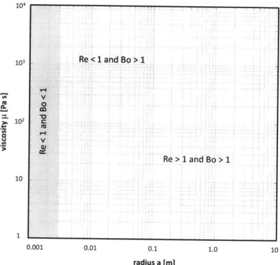
3-1 _{Dependence of the three main non-dimensional domains on bubble}

radius and magma viscosity. We assume a magma density of pf = 3500

kg/m3 and a surface-tension coefficient of o- = 0.3 N/m. The boundary

of regime 1, characterized by spherical bubbles and negligible inertia, is determined only by the size of the bubbles, because Bo does not depend on magma viscosity (see eq. 3.13). Regime 2, in which bubbles become deformable but inertia remains negligible, only exists at sufficiently high viscosity, p > 3 Pa-s. . . . . 79

3-2 Wavelength-dependence of the growth rate n over a wide range of

magma viscosities if = _{1, 10, 100, and 1000 Pa-s. The other}

pa-rameters used in the computation are pf = 3500 kg/m 3_{, pg = 1.226} kg/m 3, g = 9.81 m/s 2

, and o = 0.3 N/m. The vertical grey line

de-limits the stable size range a < _{Acr. The grey dots indicate the fastest}

growing wavelength for a specific pf from the approximative expression for Amax (eq. 3.19) that is only valid at large viscosities. . . . . 83

3-3 Overview of the non-dimensional regime covered by the 95 simulations

(black dots) constraining the stability of isolated gas bubbles at Re > 1 (sec. 3.4.2). The grey shading delimits the domain in which we observe breakup in two dimensions. A comparison with the shape regimes for bubbles during buoyant ascent [95] confirms that we reproduce the expected steady-state shape correctly in our computations. Note that we did not perform simulations for low Bo and high Re, because that case is of little relevance for basaltic magmas. . . . . 88

3-4 Breakup modes of an initially spherical bubble in two dimensions. A: An initially spherical bubble reaches its steady-state shape without breakup (Re - 5, Fr = 0.4, We a 90, and I1 = 10-6). The snapshots

shown are at non-dimensional times t = 0, 1.97, 3.93, and 5.90. B: Gradual breakup during which three small bubbles are torn off each side. The run is characterized by Re - 25, Fr = 0.3, We 800 and

n1

by Re a 250, Fr = 0.16, We ~ 1350 and H1 = 10-6. Snapshots are at

t = 0, 0.59, 1.03, 1.58, 1.91, 2.04, 2.26, and 2.49. The grid resolution

in all runs is 80 x 160.. . . . . . . . . 92

3-5 Catastrophic breakup of an initially spherical bubble in three

dimen-sions. Re ~ 16, Bo ~ 1150, and 1 i = 10-6. It is likely that, analogous

to Fig. 3-4C, a series of small bubbles is generated during catastrophic breakup in three dimensions, but not resolved due to resolution re-strictions. The computation was performed with a grid resolution of

75 x 75 x 50 equidimensional cells. The snapshots shown refer to t =

0,

3-6 Dependence of the breakup time tB on bubble radius a for gradual

breakup. In order to evaluate the dependence of tB, the computation is dimensional with pf = 3500 kg/m 3_{, pg = 1.226 kg/m} 3_{, g = 9.81}

m/s2 a = 0.3 N/m, pf = 10 Pa-s, and pg = 10-5 Pa.s. The breakup

time is expressed in percent of the initial breakup time at a = 5.4 cm. The numerical data points are associated with an error bar reflecting the finite time step At in the computation. The line represents a cubic fit through the data. ... ... 96

3-7 Overview of the non-dimensional regime covered by 52 simulations (black dots) investigating the effect of multibubble interactions on breakup at Re > 0 (sec. 3.4.3). The computations have been binned based on their initial conditions, where 1.1 112 2.

0,

while coalescence and breakup commonly occur in sequence at Re > 0, coalescence dominates at small Re and breakup at large Re. . . . . . 96

3-8 A three-dimensional computation of two deformable bubbles coming

into close contact without coalescing. Non-dimensional numbers are Re a 2, Bo a 166, 11 = 10-6, 12 = 1.43, 113 = 1.2, and H4

=

is 50 x 50 x 80... . . . . . . ... 98

3-9 A and B: Two breakup sequences as a consequence of differing initial

separation distances in the vertical direction 114 = 2 (A) and H4 1.8

(B). Both computations are based on Re ~ 5, Fr a 0.2, We 70,

i1 = 10-6, 12 = 1.43, and 13 = 1.16. The snapshots shown for the

first computation (top) refer to non-dimensional times t = 0, 1.5, 3.0,

4.5, and 6.0. Those on the bottom to t = 0, 2.32, 3.48, 4.41, and 5.80. C: Multi-bubble interactions for bubbles in the unstable size range (sec. 3.5.1). Non-dimensional numbers are Re a 350, Fr ~ 0.2, We ~ 3000, H1 = 10-6, H2 - 1.43, 113 = 1.16, and 114 = 2. Snapshots are at

non-dimensional times t = 0, 0.34, 0.51, 0.64, and 0.87. Initially, the

deformation of each bubble is reminiscent of the breakup sequence of isolated bubbles (Figure 3-4). The presence of the other bubble only becomes apparent during the late stages of breakup, indicating that unstable bubbles break up more rapidly than they interact. All three computations are based on a grid resolution of 100 x 200. . . . . 100

3-10 Overview of the non-dimensional regime covered by 69 simulations

(black dots) to constrain the stability of gas slugs (sec. 3.4.4). For all computations Hi = 10-6 and H = 0.7. The grey shading delimits

the domain in which we observe breakup in two dimensions. . . . . . 102

3-11 A: Gradual breakup analogous to Fig. 3-4B. Re ~ 10, Fr ~ 0.14,

We 95, 1 = 10-6, and 115 = 0.67. The snapshots shown are

at t 0, 0.30, 0.60, 0.90, 1.20, and 1.47. B: Gradual breakup may occur cyclically. Re a 50, Fr ~ 0.16, We ~ 100, H1 = 10-6, and H5 = 0.67. Snapshots are at t = 0, 0.94, 1.33, 1.56, 1.93, and 2.20. C:

Catastrophic breakup with gradual breakup occurring simultaneously along the walls. Re ~ 80, Fr ~ 0.10, We ~ 3000, H1 = 10-6, and

H5 = 0.7. The snapshots shown are at t = 0, 0.29, 0.59, 0.88, 1.18,

and 1.47. All three computations were performed at grid resolutions

of80 x 240. ... ... 104

3-12 Dependence of the steady-state shape of conduit-filling slugs on Re. All computations are based on a spherical initial condition and H5 =

0.7. At finite Re, a dimple forms at the rear of the slug visible on all

three interfaces. As Re increases from left to right, the steady-state width of the slug increases and the magmatic films separating interfaces and conduit walls are thinned out. Shear stresses will intensify as the magmatic films thin out and eventually lead to the tearing-off of small droplets similar to gradual breakup of isolated bubbles (Fig. 3-4B). . 106

4-1 Comparison of the slug and plug model. A: The slug model assumes that the volcanic conduit is filled with fluid magma (grey) throughout. Each Strombolian eruption is thought to represent the burst of a gas slug of up to 35 m3 [226]. B: Instead of focusing on one vent, the plug model captures

the dynamics of the entire crater terrace. It incorporates the dichotomy of Strombolian magma with HP magma residing at shallow and LP magma at large depth. Flow in the LP magma is driven by buoyant ascent of gas bubbles inducing convective flow in the magma. For the first few hundred meters below the free surface, HP magma is crystalline enough to behave

as a porous plug at low shear and strain rates. . . . . 112

4-2 Illustration of the rheological transitions with increasing crystal fraction. Estimates of melt strength are computed by viscosity x strain rate. At zero to low crystal fraction, the aggregate is fully liquid (regime A), where the increase in effective viscosity is given by the Einstein-Roscoe relationship. In the transitional regime, B, it is partly liquid and partly solid. The strength of the aggregate increases rapidly through a power-law (Bingham rheology). Beyond a rheologically critical crystal fraction, the aggregate behaves like a

solid body (domain C). . . . . 113

4-3 Increase in crystallinity with decreasing pressure at 1115'C computed with

MELTS based on the bulk composition of Strombolian magma from [80].

The shaded boxes highlight the observed crystallinity of HP magma at

Strom boli. . . . . 114

4-4 Geometry of the elliptical cylinder representing the plug with semimajor

axis a, semiminor axis b and thickness 2h. The coordinate is located at the center of the plate with z corresponding to the vertical direction. The plate is stressed at the lower surface (shaded in grey) by a uniform pressure p. . 116

4-5 Overview of the spatial distribution of maximum shear at different depth intervals inside the plug with seirniniajor axis a, semiminor axis b and moder-ate thickness h = 70 m based on the analytical solution for moderately thick

plates (Appendix C). The top panel compares the value of maximum shear at the two boundary points furthest from the center, (a, 0) and (-a, 0), the two boundary points closest to the center, (0, b) and (0, -b) and the center throughout the plug. The bottom panels show the spatial distribution of maximum shear at various depths through color shading and five iso-stress contours. All stresses are nondimensionalized by the pressure applied at the

lower surface of the plug. . . . . 118

4-6 Comparison of the increase in integrated maximum shear at the edges of

the ellipse (in percent with respect to the center of the ellipse) and the vent locations (black dots) from October 1994 to September 2002 as mapped by [104]. The size of the ellipse is adjusted to coincide with the edge of the

crater terrace. . . . . 120

4-7 The gas-driven eruption cycle suggested in the plug model. Continuous gas

accumulation underneath the plug exerts an increasing pressure onto the overlying material until the critical pressure for failure is reached. Normal eruptions represent ductile failure of the plug during which the gas-rich

layer underneath is partially drained. The buoyancy pressure drops , the

eruptions ceases and gas accumulation begins again. . . . . 121

5-1 The wetting angle 0 is the angle between the crystal face and the tangent

to the bubble surface at the point of contact. . . . .. 130

5-2 Relative supersaturations required for heterogeneous nucleation APhet as

compared to homogeneous nucleation APhom for wetting angles from 6 = 0'

5-3 Evolution of the volatile content (top) and saturation pressure (bottom) in

a 1000-km-deep magma ocean with the fluid composition derived by [107]

and initial volatile content 0.05 % water and 0.01 % carbon dioxide. The

solubility behavior is computed based on [205]. The grey domain highlights volatile enrichment levels sufficient for heterogeneous nucleation based on the uncertainty interval given in sec. 5.3.1. The inset in the bottom figure illustrates that the supersaturation pressure corresponds to a depth which

increases with increasing volatile enrichment (not plotted to scale). . . . 138

5-4 An example computation of the rate of heterogeneous nucleation J for

vari-able supersaturations of the melt AP. Nucleation becomes apprecivari-able (i.e. J > 1cm- 3s-1) at AP 210 MPa. However, in the pressure range 210 < AP < 220 MPa the nucleation rate is still too low to trigger a local shift in convective forces and thus little to no degassing is expected. The

beginning of catastrophic degassing occurs at AP

=

may be regarded as instantaneous (i.e. J > 104cm-3s-1) at AP > 224 MPa. 139

5-5 Comparison of the depth dependence of solubility for water and carbon

dioxide based on the solubility model by [205]. The melt composition is

assumed to be basaltic (as specified in Table 3, [205]) and T = 2000'C. In both cases we assume a small amount (0.01 wt %) of the other volatile

present in the m elt. . . . . 142

5-6 Overview of the two phases of magma ocean solidification that are pertinent

to catastrophic degassing sequences. Left: Nucleation delayed by insuffi-cient supersaturation and bubble breakup create small bubbles that remain entrained and do not degas. Right: Once bubbles have reached a critical sized required for degassing, compositional convection becomes dominant at shallow depths. Catastrophic degassing may not happen until > 80% solidi-fication for a 1000-km-deep magma ocean as may have existed on terrestrial

5-7 Illustration of the three end-member cases of magma ocean degassing. Note

that the wiggly arrows in red represent heat flux and not degassing. The first case (A) represents continuous degassing and gradual atmosphere formation. It applies to magma oceans with extremely high initial volatile contents or alternatively, with a content of crystals that are wetted perfectly by at least one of the dissolved volatiles. The second case (B) represents a degassing history characterized by one or several catastrophic degassing events with little or no degassing happening prior or after. Catastrophic degassing leads to the sudden formation of a substantial atmosphere. In the third case

(C), the volatile content is never sufficient to trigger degassing and little

atmosphere will form during solidification. The initial magma ocean depth is smaller in this case to reflect that this scenario is more likely for shallow

m agm a oceans. . . . . 149

6-1 Computational domain for the simplified case of a single sphere sinking in

viscous fluid. Q describes the entire computational domain including both solid and fluid phases and 80 its boundaries. P is the portion of the domain occupied by a single or multiple particles and OP is the solid-fluid interface. 156

6-2 Comparison of the wake behind a fixed cylinder at Ref = 26 as observed

experimentally (top) by [284] and computed numerically (bottom). The green arrow highlights the position of the second stagnation point in both

cases. . . . . 164

6-3 Instantaneous out-of-plane vorticity over a fixed cylinder at three different

Reynolds numbers showing Von-Kirmain-vortex shedding. . . . . 166

6-4 Convergence test for the drag on a fixed circular cylinder at Re = 40. We investigate the convergence of the viscous C, and the pressure contribution

C, to the drag on the cylinder's surface separately (see eq. 6.28 and [110]).

Despite using a second-order fluid solver, the convergence at the fluid-solid

6-5 _{Temporal evolution of drag and lift coefficients for flow over a circular}

cylin-der at four different Reynolds numbers. The grid resolution in all four cases

is 800 x 1600. _{. . . . 169}

6-6 Instantaneous out-of-plane vorticity over a square cylinder at three different

rotation angles and Re = 410 showing Von-Kirmin-vortex shedding. . . 170

6-7 Temporal evolution of drag and lift coefficients for flow over a square cylinder at Re = _{500. Contrary to the case of a circular cylinder, both drag and lift}

exhibit period doubling as previously observed by [266]. . . . . 171

6-8 Solid sphere sinking in viscous fluid at Rep = 90. The computational domain

is 3d x 3d x 9d and the resolution is 41 x 41 x 121. The local speed of the flow field is represented in colour and the contours of the stream function are shown in white. The colouring of the sphere itself indicates its speed at

a given tim e. _{. . . . 173}

6-9 _{Comparison of the predicted drag coefficient for different Reynolds numbers}

with the empirical relationship by [50]. . . . . 174

6-10 The four stages of the interaction mode drafting-kissing-tumbling observed

for two identical spheres at finite Re. The approximate Re of the

computa-tion is 150 based on the maximum settling speed of the spheres. . . . . . 175

7-1 _{Convective regimes in a solidifying magma ocean. At the planetary scale}

flow is driven by thermal convection. Flow is turbulent for most of the depth range of the magma ocean except for a boundary layer at the bottom where flow is rapid but non-turbulent. The conductive boundary layer is not vi-sualized. The degree to which crystals can settle out of suspension in the steady-flow regime at the bottom of the magma oceans depends on the lo-cal fluid-dynamilo-cal conditions and is therefore dominated by compositional

7-2 Body centered cubic (bbc) particle array consisting of spheres with radius

r. In this staggered setup, the smallest gap between particles is given by g. The side length of the cell is given by a; a reasonable proxy for a typical

separation distance of the crystals... . . . . . . . 183

7-3 Drag coefficient CD for a sphere (3D) from 1 < Rep 1000 based on the

data by Clift et al. (1978). The Stokes drag law, more precisely its Oseen

extension [50] is also plotted for comparison purposes. . . . . 185

7-4 Simultaneous settling of 30 identical crystals with Rep

a

field at times 0.6s, 1.05s, 1.65s, 2.25s, 3.9s and 4.5s. The influx speed is set to the equilibrium settling speed of an isolated crystal in stagnant fluid. Since the presence of other crystals increases the drag experienced by each single crystal, the crystals tend to drift backwards over time. The color shading represents the average local flow speed normalized by the influx speed and the white contour lines represent the out-of-plane vorticity. The

computations was done at a grid resolution of 800 x 1600. . . . . 187

7-5 Temporal evolution of the drag (top) and lift (bottom) force for 30 identical

spherical crystals (see Fig. 7-4) normalized by the drag and lift forces in the very dilute limit. The thick red line represents the mean drag and lift

at a given tim e. . . . .. 189

7-6 Simultaneous settling of 5 heavy crystals (Rep 120) amidst 30 light

crys-tals (Rep 80) in a linear flow field at times 0.38s, 0.9s, 1.5s, 2.25s, 3.75s

and 4.5s. The influx speed is set to the equilibrium settling speed of an iso-lated grey crystal akin to Fig. 7-4. The color shading represents the average local flow speed normalized by the influx speed and the white contour lines represent the out-of-plane vorticity. The computations was done at a grid

resolution of 800 x 1600. . . . . 190

7-7 Temporal evolution of the drag (top) and lift (bottom) force for the 30

grey crystals (blue and green, respectively) and the 5 black crystals (red) as shown in Fig. 7-6) normalized by the drag and lift force of a single sphere

7-8 Average linear momentum of 5 and 7 heavy spheres (Rep 120) settling

amidst 30 and 42 light crystals (Rep 80) at initial separation distances

a = 10r and a = 7.5r. Spikes in the curve represent rapid changes in

momentum due to crystal collisions. Arrows indicate the onset of collisions

for either case. . . . . 192

7-9 Two simulations of 30 spheres with equal density but variable size. In both

cases, the influx is identical to Figs. 7-4 and 7-6 and the total crystal fraction is identical to Fig. 7-4 to within 0.001 %. Contrary to the case of a homogeneous crystal-size distribution, the crystals begin to segregate immediately. Run A (snapshots are taken at times 0.38 (Al), 1.50 (A2), 3.00

(A3), and 4.51 (A4))is characterized by a smaller deviation in crystal sizes

and therefore separation of the crystals is slower than in case B (snapshots are taken at times 0.38 (B1), 1.13 (B2), 3.00 (B3), and 4.13 (B4)). The

computations was done at a grid resolution of 800 x 1600. . . . . 193

7-10 Illustration of the entrainment of a small dense crystal (black) in the wake

of a large and less dense crystal (grey). The settling of the large crystal dominates the local flow field sufficiently to divert the small crystal without colliding with it. The snapshots are details from the computation shown in

F ig. 7-11. . . . . 195

7-11 Simultaneous settling of 5 heavy crystals (Rep 120) amidst 30 light

crys-tals with a linear crystal-size distribution in a linear flow field at times 0.38s, 0.90s, 1.50s, 2.25s, 3.00s, and 3.75s. The influx speed is identical to Fig. 7-4 and 7-6. The color shading represents the average local flow speed normalized by the influx speed and the white contour lines represent the out-of-plane vorticity. The computations was done at a grid resolution of

800 x 1600. ... ... .. .... .... .. 197

7-12 Depth dependence of adiabat, liquidus and solidus for Vesta, the Moon and

7-13 Relationship of the crystal-size distribution slope to the time variation in

nucleation rate [180]. The top row (A) describes a single nucleation event and the middle row (B) a sequence of two nucleation events leading to a kinked crystal-size distribution. The bottom row (C) represents the hy-pothesized origin of skewed crystal-size distributions in solidifying magma

oceans due to numerous nucleation events that are closely spaced in time. 204

A-1 Numerical (left) and analytical (middle) solution for the pressure field for

benchmark problem 2. The viscosity contrast between inclusion and sur-rounding matrix is 6 (top row) and 10 (bottom row) orders of magnitude. The right panels shows the percentage error for both computations. The

grid resolution is 150 x 150 in both cases. . . . . 215

A-2 Convergence test for benchmark problem 3. Shown are the numerical

solu-tions for the pressure jump due to surface tension at the interface between a viscous drop and the surrounding fluid at grid resolutions 21 x 21 (left),

31 x 31 (center), and 41 x 41 (right). Each dot represents one grid point.

Although the jump as such is resolved sharply without artificial smoothing at all of these resolutions, a minimum of ~~ 15 grid points in both the x-and y-direction are required inside of the drop to resolve its spherical shape. 216

A-3 Convergence test for benchmark problem 2. The viscosity contrast is I1, = 10-3 as discussed in the paper, sec. 2.5.2. The shown grid resolutions are

20 x 20 (top) and 80 x 80 (bottom). In both cases, we contrast numerical (left) and analytical solution (right). The comparison shows that the addi-tional challenge of benchmark problem 2 as compared to benchmark problem 1 lies in fully resolve the magnitude of the pressure jump, for which high

A-4 Left: Convergence test for the isothermal and isoviscous Rayleigh-Taylor instability, benchmark problem 3. A lack of convergence is easiest to identify during the phases of rapid rise of an instability. We illustrate this for the rise of the secondary instability on the right side of the box at time t=1000 and four different grid sizes: 60x66, 80x88, 100x110, and 120x132. We observe convergence for grid sizes above 100x 110. Right: Convergence test for the isothermal and isoviscous Rayleigh-Taylor instability, benchmark problem 3. Analogous to Fig. S7, we illustrate this convergence test for the rise of the secondary instability at time t=1000. The four interfaces were

computed based on the time steps: At = _{180Ax, At = 90Ax, At = 45Ax,}

and At = 25Ax. We observe convergence for time steps At ; 25Ax. . . . 218

A-5 Illustration of the accumulation of numerical error over time reflected in

mass fluctuations. The plot shows the mass of the buoyant phase as a per-centage of its initial mass. This plot compares to a similar plot presented

by Schmalzl and Loddoch, [2003]. We note that fluctuations < 1% are not

unexpected in complex fluid dynamical simulations. Overall, the mass con-servation is satisfactory. . . . 219

A-6 Illustration of the potential bias introduced through an iterative

reinitial-ization procedure. The left figure (A) shows the isothermal and isoviscous Rayleigh-Taylor instability at t=1500 computed with extension velocities. The other two figures (B) and (C) are based on an iterative reinitialization procedure, but different parameters are used in the iteration. For case (B) a single reinitialization iteration is performed at each computational time step At and AT = _{0.9Ax is used in the numerical solution of equation A.16.}

For case (C) 20 iterative reinitialization steps were taken at each physical

time step At with AT = 0.9Ax/20. All computations were performed on a

A-7 The Rayleigh-Taylor instability as computed by the HS-tracer method at

time t=1500. The equations of motion for this simulation were solved on an 81 x 81 grid. The right panel is a zoom onto the peak located left of the descending instability. Each blue dot represents one particle and the grid represents a rough estimate of the scale at which the flow field is

approxi-m ated correctly. . . . . 221

B-1 Dependence of the breakup time tB on bubble radius a for large bubbles. In

order to evaluate the dependence of tB, the computation is dimensional with the same parameters as in Fig. 3-6: pf = 3500 kg/m3, pg = 1.226 kg/m 3, g = 9.81 m/s2

, o. = 0.3 N/m, If = 10 Pa-s, and pig = 10-5 Pa.s. The

breakup time is expressed in percent of the initial breakup time at a = 5.4 cm. The numerical data are no longer compatible with the simple scaling relationship tB ~ a3 (eq. 3.20), which is not unexpected, given the wide

fluid dynamical range it spans. . . . . 224

B-2 Dependence of multibubble interactions on the initial vertical separation distance. The three simulations show two bubbles passing (top), breaking

up (middle), and coalescing (bottom) as a consequence of increasing the

non-dimensional vertical distance 113 = 1.16 (top),

H3

H3 = 1.4 (bottom). The other non-dimensional numbers are identical for

the three simulations: Re ~~ 5, Fr ~ 0.2, We ~ 70, Hi= 10-6, 112 = 1.43, and 114 = 2. Snapshots are taken at non-dimensional times t = 0, 1.5, 3.0,

4.5, and 6.0. All three computations were performed with a grid resolution

of 100 x 200. ... ... .... 226

B-3 Convergence test for the catastrophic breakup of an isolated gas bubble (compares to Fig. 3-4C). Shown are four computations at differing

resolu-tions 40x80, 80x160, 160x320, and 320x640. . . . . 228

B-4 Convergence test for the catastrophic breakup of a conduit-filling gas slug (compares to Fig. 3-11C). Shown are four computations at differing

B-5 Convergence test for the gradual breakup of an isolated gas bubble (com-pares to Fig. 3-4B). Shown are four computations at differing resolutions

40x80, 80x160, 160x320, and 320x640. ... ... 229

B-6 Convergence test for the gradual breakup of a conduit-filling gas slug (com-pares to Fig. 3-11A). Shown are four computations at differing resolutions

40x80, 80x160, 160x320, and 320x640. ... ... 230

C-1 Thin-section analysis of Stromboli's HP magma. . . . . 232

C-2 Left: Maximum shear stress for a thick elliptical cylinder overlain by the

computational grid generated by Distmesh. The stresses are extremely high in the vicinity of the side boundaries. Right: Maximum shear stress for a

thick elliptical cylinder with a free-moving side flank. . . . . 237

C-3 Stress concentration around the bubble interface in a purely extensional

stress field. The stress is measured in multiples of the applied stress at

the boundary Obc. The black circles surrounding the bubbles correspond to

three times the radius of the bubble and denote the range over which the stress concentration due to the presence of the bubble is appreciable (Saint-Venant's principle). In panel A, the bubbles are spaced closely enough for substantial stress concentration; in panel B, the bubbles are far enough apart to be negligible on the large scale. The purely compressional case is

analogous. .. . . . . . . . 238

D-1 Illustration of the activation energy for homogeneous nucleation. The blue

curve represents the Free Helmholtz energy AFsurf required for forming a new interface and the red curve the volumetric gain in Free Helmholtz energy

AF,,l from the presence of a bubble. The sum of the two contributions is

shown in green. An activation energy of AF* needs to be overcome for

spontaneous nucleation to occur. . . . . 240

List of Tables

2.1 Analytical versus numerical results for the pressure jump due to surface tension at the interface of a static drop. This computation was done dimensionally with o- = 0.0728 kg/s 2 - a representative value for the air/water interface. . . . . 59

2.2 Comparison of the quantitative parameters characterizing the dynam-ics of the isoviscous Rayleigh-Taylor instability. . . . . 64

3.1 Theoretical prediction of the maximum stable bubble radius ama,, in basaltic magma of different viscosities pf. Additional parameters used in the computation: pf = 3500 kg/m3_{, pg = 1.226 kg/m} 3_{, g}

= 9.81

m/s 2

, surface tension o = 0.3 N/m, and viscosity ratio 10--6. ... 87

5.1 Overview of variables used in the text. . . . . 128

5.2 Supersaturations required for non-zero homogeneous (eq. D.3) and het-erogeneous (eq. 5.3) nucleation in a basaltic magma ocean with vari-able volatile contents. We consider nucleation rates of J < 1 cm-3

s1- to be negligible. The remaining parameters are o = 0.3 N/m,

= 3400 kg/m3_{, T = 1100K, g = 9.5 m/s}2_{, VH} 20 11.5A 3_,

Vco

4A

_,

_[326],

_D

/s [315, 326, 313]. In order to take both water and carbon

diox-ide into account for the computation of the forefactor Jo, we take the weighted mean of the parameters characterizing water and carbon diox-ide, respectively . . . . 137

5.3 Overview of expected bubble sizes in a magma ocean including their dynam ical behavior. . . . . 141

6.1 Mean drag coefficient CD for flow over a circular cylinder at different Reynolds numbers based on the simulations in Fig. 6-5. . . . . 167

6.2 Strouhal numbers for flow over a fixed cylinder at different Reynolds numbers based on the simulations in Fig. 6-3. . . . . 167 6.3 Mean drag coefficient CD for flow over a square cylinder. . . . . 172

7.1 Order-of-magnitude estimates for the key non-dimensional parameters characterizing flow in magma oceans. . . . . 178

7.2 Approximate physical parameters for a theoretical magma ocean. . . 178

7.3 Overview of different types of suspensions grouped according to the crystal fraction and the corresponding non-dimensional gap between crystals as defined in Fig. 7-2. . . . . 183

Chapter 1

Introduction

This dissertation consists of six self-contained studies linked together through their focus on multiphase flow problems and their computational methodology. Broadly speaking, all fluid systems in which different liquid, gaseous or solid phases are si-multaneously present may be considered multiphase. Without further specification, however, nearly all of fluid dynamics would fall under this generic label. In the sense in which the term multiphase flow is commonly used, it denotes a more specific class of problems typically tied together by the context in which they arise rather than

by an abstract similarity in their properties. This thesis is no exception: The

com-monality of the multiphase systems investigated here is their relevance for magmatic

flow.

A large number of problems in Earth science are related to the solidification

pro-cesses in molten rocks. Examples range from the propagation velocity of hazardous lava flows to the differentiation of cooling magma oceans and the disputed origin of layering in igneous intrusions. We are well equipped to model the two end-member cases of the solidification process, i.e. the early stages in which the aggregate is largely molten and the final stages in which it is mostly solid. The greatest challenge is posed

by the intermediary stages in which crystallized minerals, exsolved gas bubbles and highly viscous magma may all contribute significantly to the dynamics of the

aggre-gate. The goal of this thesis is to extend the reach of our numerical models a little further into this complex regime of solid-fluid-gas interactions.

Much of the complexity of modeling multiphase flow stems from the dynamic inter-action of the various fluid and solid phases that are simultaneously moving through the system. This complexity limits the usefulness of purely analytical approaches. Laboratory experiments provide a compelling alternative, but may not always offer the necessary degree of control over the length scales and the physical parameters characterizing the flow. Numerical simulations are thus an essential complement to experiments and, for certain problem, they may be the only available tool for inves-tigating multiphase dynamics.

Computational methods for multiphase flows are as varied as the problems for which they are intended. Here we consider a class of approaches that are commonly referred to as direct numerical simulations. These types of methods are direct in the sense that they fully resolve the physics of the problem from first principles instead of relying on effective constitutive laws, approximate settling speeds, or similar simpli-fying assumptions. Direct numerical simulations are thus particularly advantageous for complex flow problems for which it is typically not possible to specify effective ensemble properties a priori.

The added sophistication of fully resolving the fluid dynamic interaction of all suspended phases limits the reach of direct numerical simulations to length scales commensurate to the length scales of the interfaces in the flow. Particularly in the Earth sciences, where the relevant flow systems may span whole planets, this limitation highlights that direct numerical simulations are a complement to more traditional approaches such as large-scale convection simulations rather than an al-ternative. They offer the possibility to gain more detailed insights into the complex fluid-dynamical interactions at small scales and can thus inform the inputs required for large-scale computations such as rheology, effective viscosity or settling velocities

of suspended particles.

Another role that direct numerical simulations may play in Earth science is to help forge a closer connection between petrological observations and numerical models. In-tegrating data on the bubble content, the types of mineral phases or the crystal size distribution characterizing a given flow system into geodynamical models has proven

challenging, because the physical ramifications of these observations are often not obvious. Direct numerical simulations may shed some light on these complex con-nections and thereby contribute to creating a tighter link between field observations, experiments and modeling.

This thesis studies the potential of direct numerical simulations for advancing our fundamental understanding and predictive capabilities of the multiphase dynamics of cooling magmatic flow. This task implies both a methodological and an applied focus. The usefulness of direct numerical simulations is inevitably tied to the insights that these computations can reliably provide for complex three dimensional systems. The choice of numerical scheme has a profound influence on the tractability, accuracy, robustness, and efficiency of the simulation. Even a state-of-the-art numerical model, however, is useless if it does not make a significant contribution to our understanding of some of the important open questions in Earth science.

Here we discuss two specific examples in which the results from direct numer-ical simulations provide a new perspective. The first example is the dynamics of an exsolved gas phase ascending in basaltic lava, which is critical for understanding the mechanism of explosive eruptions in basaltic volcanoes. The key methodologi-cal challenge in this suite of computations is the accurate treatment of the rapidly deforming interface between two fluids, gas and magma, with drastically different viscosity. The second example is crystal settling in cooling magma oceans, which is essential for constraining the later evolution of the planet including the onset of convective overturn and early volcanism. The key methodological challenge for this series of simulations is the full dynamic coupling of solid and fluid phases for various densities, shapes and crystal size distributions. The thesis is broadly divided into two parts by the discussion of basaltic volcanism (chapters 2- 4) and planetary evolution (chapters 5- 7).

In chapter 2 we develop and benchmark the computational methodology for fully resolving the interface dynamics of buoyancy-driven flow in the presence of large viscosity contrasts. Our implementation relies on the combination of three numerical methods, an extended ghost fluid type discretization which we extend to the Stokes