Dynamic Energy Budgets and Bioaccumulation: A Model for
Marine Mammals and Marine Mammal Populations
by
Tin Klanjsek
Dipl. Ing. Physics, University of Zagreb, Croatia (2000)
Submitted to the Department of Biology in partial fulfillment of the requirements for the degree of Doctor of Philosophy in Biological Oceanography
at the
MASSACHUSETTS INSTITUTE OF TECHNOLOGY and
WOODS HOLE OCEANOGRAPHIC INSTITUTION June 2006
ARCHpvIES
©Tin Klanjek
The author hereby grants to Massachusetts Institute Oceanographic Institution permission to reproduce and document in whole or in part.
of Technology and to distribute copies Woods Hole of this thesis Signature of Author ... A\
Certified
by...
Certified
by
... ...
Ai Accepted by .... Department of Biology ! r 27 *bril 2006 Hal Caswell Senior Scientist, WVHOIThesis ,Supervior
Michael G. Neubert ssociate Scientist, WHOI
. Thesis Spervisor
. . . ... . . . .' I. . . . .d'o~ nEd long
Chairman, MIT/WHOI Joint Committee on Biological Oco aphy
JUN 0 9 20
MACHUSETTS NSTV UTEE
-OF TECHNOLOGY
-
Dynamic Energy Budgets and Bioaccumulation: A Model for
Marine Mammals and Marine Mammal Populations
by
Tin Klanjsek
Submitted to the Department of Biology
in partial fulfillment of the requirements for the degree of Doctor of Philosophy in Biological Oceanography
Abstract
Energy intake of individuals affects growth of organisms and, therefore, populations. Persistent lipophilic toxicants acquired with the energy can bioaccumulate
and harm individuals. Marine mammals are particularly vulnerable because of their large energy requirements, and transfer of energy and toxicants from mothers to their young during gestation and lactation. Dynamic energy budget (DEB) models for energy assimilation and utilization, coupled with pharmacokinetic models that calculate
distribution of toxicants in individuals, can help investigate the vulnerability.
In this dissertation I develop the first individual DEB model tailored specifically to marine mammals and couple it to a pharmacokinetic model for lipophilic toxicants. I adapt the individual model to the right whale and use it to analyze consequences of energy availability on individual growth, reproduction, bioaccumulation, and transfer of toxicants between generations.
From the coupled model, I create an individual-based model (IBM) of a marine mammal population. I use it to investigate how interactions of food availability, exposure to toxicants, and maternal transfer of toxicants affect populations. I also present a method to create matrix population models from a general DEB model to alleviate some of the drawbacks of the IBM approach.
Thesis Supervisor: Hal Caswell Title: Senior Scientist, WHOI
Thesis Supervisor: Michael G. Neubert Title: Associate Scientist, WHOI
Acknowledgements
I will forever be grateful to my advisors, Hal Caswell and Michael G. Neubert, for the freedom I had in choosing my research topic, and their guidance. I am equally grateful to Roger M. Nisbet for dynamically guiding me through the budgets of energetics and hosting me in California. I owe a debt of gratitude to Michael Moore for his ifs and buts on every simplification of marine mammal physiology I suggested, and Mark Hahn and Eric Montie for their help with toxicological aspects of my work. I would also like to thank Daniel Rothman for our discussions that contributed to my understanding of scaling in ecology, and ecology in general.
My friends and the Falmouth community made this alien feel at home. I would like to thank them for their friendship and support; Ivek Ceraj, Vanja Klepi-Ceraja, Beckett Coppola, Michael Desai, Kristin Gribble, Ivona Josip-Ovic, Petra Klepac, Joy Lapseritis, Gareth Outlawson, Enrique Montie, the Muldoon family, Sheri mrs. Michael
Simmons, and - last only because the alphabet says so - David Stubinator, thank you. Also, big thanks to my labmates Masami Fujiwara and Christine Hunter for their help and tolerance of the 'creative disorder' on my desk. Jenny, thank you for
understanding that a thesis cannot be written in a day.
Julia, Marsha and Laishona, thank you. Please find the strength to change the things you can, the serenity to accept the things you cannot, and the wisdom to know the difference.
Most importantly, I'd like to thank my family -mom, dad, Gaga, baka Kata, baka Jasminka, deda Joza, deda Dali, Vlatka, Karlo and teta Mirka- who have supported me emotionally and financially throughout my student life. The MIT/WHOI joint program was only the last step in their efforts to educate me the best they can despite my objections. I lack the words to describe my gratitude.
This work has been supported by the David and Lucile Packard Foundation, the US National Science foundation (DEB-9973518 and OCE-0083976), the US
Environmental Protection Agency (R-82908901-0), the National Oceanographic and Atmospheric Administration (NAO 3NMF4720491) and theWHOI/MIT Joint Program in Oceanography.
Contents
1 Introduction
1.1 Thesis outline ... 1.2 References ...
2 Energetics and toxicant
mals 2.1 Abstract ... 2.2 Introduction... 2.3 Model Description 2.3.1 Energetics . . 2.3.2 Pharmacokinet 2.4 The Right Whale . .
2.5 Results...
2.5.1 Growth and reproduction 2.5.2 Toxicant distribution and 2.6 Discussion ...
2.7 Acknowledgements ...
2.8 References ...
2.9 Appendix ... 2.9.1 Morphometrics ....
bioaccumulation: a model for marine
mam-. . . . .. .. . .. . . . .o . . . . . . . . . o . .. . . . . ics . . . . . . . .. . . . .. . . . . vertical . . .. . . . . . . . . .. . . . .. . . . . . . . . . . . . . . . . . . . . . . . . . transfer . . . . . . . . . . . . 2.9.2 Energetics 13 18 21 25 25 26 29 33 41 44 45 45 53 58 66 66 77 77 . . . 79
...
...
...
...
...
...
...
...
...
...
...
...
...
...
...
...
2.9.3 Pharmacokinetics (DLS and CI) ... 85
3 Bioaccumulation and effects of exposure in marine mammal popu-lations 87 3.1 Introduction . ... 87
3.2 Methods ... 90
3.2.1 Individual energy budget and pharmacokinetic model ... 90
3.2.2 Modelling mortality . . . 94
3.2.3 Characterizing bioaccumulation ... . 97
3.2.4 The individual-based model . ... 98
3.3 Results ... 103
3.3.1 Effects of exposure on bioaccumulation and population growth rate ... . 105
3.3.2 Effects of maternal transfer on bioaccumulation and effects of exposure ... 107
3.4 Discussion . . . 114
3.5 References ... 118
3.6 Appendix A - values used in figures ... ... . 122
3.6.1 Figure 3-5 . . . 122
3.6.2 Figure 3-6 . . . 124
3.6.3 Figure 3-9 . . . 126
3.7 Appendix B: Model code . . . 127
4 Integrating Dynamic Energy Budgets into Matrix Population Mod-els 155 4.1 Abstract ... 155
4.2 Introduction ... 156
4.2.1 The DEB model ... 157
4.3 Methods ...
4.3.1 Maturation probability () .... 4.3.2 Survival probabilities (a) ... 4.3.3 Fecundity (F) ...
4.3.4 The individual-based model (IBM) 4.4 Results. ...
4.4.1 Long term (asymptotic) dynamics . 4.4.2 Seasonal environmental variability. 4.4.3 Short term (transient) dynamics . . 4.5 Discussion ... 4.6 Acknowledgments. ... 4 7 Rforanrcx 4.8 4.9 4.10
...
164
...
164
...
165
...
166
...
167
...
169
...
169
...
178
...
180
...
182
...
185
- .... . . . .. .. . . .. . .· Appendix A: Creating a matrix model based on a physiological Appendix B - Calculating the stable age distribution ... Appendix C - The extended matrix population model ... 4.10.1 Transitions between size classes, R(k) ...ji . . . . 4.10.2 Transitions between energy classes, Q(f) ... 4.10.3 Calculating the projection matrix ... 4.10.4 Preliminary results ... 4.10.5 Seasonal variability .......
185
model 189....
190
....
192
....
193
....
195
....
196
....
197
....
197
205 212 5 Conclusion 5.1 References . . . . · .8List of Tables
2.1 Compartments and state variables with units. 2.2 Equations for the energy fluxes ...
2.3 Kinetics: rates of change of state variables..
2.4 Right whale parameter values. ...
3.1 Compartments and state variables with units.
3.2 Kinetics: rates of change of state variables. . . 3.3 Equations for the energy fluxes ...
3.4 Right whale parameter values. ...
3.5 Figure 5: 3.6 Figure 5: 3.7 Figure 5: 3.8 Figure 5: 3.9 Figure 6: 3.10 Figure 6: 3.11 Figure 6: 3.12 Figure 6: 3.13 Figure 9: 3.14 Figure 9: 3.15 Figure 9: Growth rate ... CB ... . .. . . .. Reproductive probability ....
Var(CB)...
... . . . 122 122 123 123 Influence of maternal transfer on the population growth rate 124 Influence of the maternal transfer on CB ... . 124Influence of maternal transfer on the reproductive probability 125 Influence of maternal transfer on the variance of CB .... 125
Asymptotic
CB
. . . . .126
Introduction rate of the toxicant into the population ... 126
Depuration rate of the toxicant from the population ... 126
4.1 Standard parameter values ... ... 159
30 31 31 32 93 93 93 94
4.2 State variables as a function of age (s) and parameters of the DEB model. For further discussion see Kooijman (2000) ... ... . 160 4.3 Transition counts nij from stage j to stage i . ... . 169 4.4 Comparison of predicted and observed demographic statistics and vital
rates ... 170
List of Figures
2-1 Marine mammal model outline ... 30
2-2 Length of non-reproducing right whales as a function of age for different food availabilities . . . 47
2-3 Influence of reproduction on growth ... ... . 48
2-4 Calving interval and age to maturity for a range of food availabilities 50 2-5 Lifetime energy and toxicant distribution for a reproducing female. 51 2-6 Male and female toxicant bioaccumulation in constant and seasonally varying environments . . . .. 56
2-7 Toxicant transfer as a function of birth order ... 57
2-8 Effects of biotransformation ... 59
3-1 Simplified individual model outline ... ... . 92
3-2 Flowchart of the main steps in the simulations ... 101
3-3 Measuring the convergence of the age distribution . ... 102
3-4 One simulation of the individual-based model ... ... . 104
3-5 Effects of exposure on population growth rate and bioaccumulation.. 106
3-6 Effects of maternal transfer on population growth rate and
bioaccumu-lation...
108
3-7 Bioaccumulation with and without maternal transfer ... 109
3-8 Transient response of bioaccumulation to changes in the toxicant con-centration in the environment ... 112
4-1 The fluxes of energy in a n-rule DEB model ... 158
4-2 Sample solutions of the DEB model ... 159
4-3 Schematic of the assessment process ... 167
4-4 Predicted and observed vital rates and demographic statistics versus
ageing
acceleration
(ha)
.
. . . .171
4-5 Predicted and observed vital rates and demographic statistics versus energy intake (f) ... 172
4-6 Predicted and observed vital rates and demographic statistics versus cost of a newborn (CN) . . . . 173
4-7 Predicted and observed vital rates and demographic statistics versus maximum energy density ([Em]) ... ... . 174
4-8 Predicted and observed vital rates and demographic statistics versus energy allocation ratio () ... 175
4-9 Predicted and observed vital rates and demographic statistics versus age to maturity ... 176
4-10 Predicted and observed vital rates and demographic statistics versus amplitude of sinusoidal food intake fluctuations (fA) ... . 179
4-11 Population response to colonization and to a catastrophe ... . 181
4-12 Two food intake scenarios . . . 199
4-13 Growth rate in a seasonally varying environment ... . 200
4-14 Minimum growth rate as development time increases. See text for discussion ... 201
4-15 An example of a periodic environment ... 202
4-16 Growth rate as a function of variability and amplitude of environmental fluctuations ... 203
Chapter 1
Introduction
It isn't pollution that's harming the environment. It's the impurities in our air and water that are doing it.
(Unknown)
Marine mammals are awe-inspiring creatures. Many whales traverse the oceans, and blue whales (Balaenoptera musculus) are the largest creatures on the planet. They communicate across tens, possibly hundreds of miles (Dudzinski et al. 2002), hold their breath for hours, dive to depths of more than 2000m (Stewart 2002), coordinate their behavior, and socialize (Tyack 2002). As many other wild species, they are threatened by human influence: humans compete with them for food and space, hunt them, and pollute their environment. As early as 1972, the US Congress concluded that "certain species and population stocks of marine mammals are, or may be, in danger of extinction or depletion as a result of man's activities", and that "such species and population stocks should not be permitted to diminish beyond the point at which they cease to be a significant functioning element in the ecosystem of which they are a part" (Marine Mammal Protection Act 1972). Understanding marine mammal population dynamics and how it is affected by human interaction is crucial to that goal.
Since 1925 (Lotka 1925, Volterra 1926), mathematical models have been gaining in popularity as a tool to investigate population dynamics; today, they are widely accepted and utilized. Every mathematical model of a population has to span scales of biological integration by connecting processes of individual growth, reproduction and mortality to population dynamics. The environment and interactions with other
species affect these processes and, consequently, population dynamics.
The most prominent environmental factors affecting individual growth, reproduc-tion and mortality include food availability and toxicants. Available food, and the resulting energy intake profoundly affect growth and reproduction. Since toxicants are often bound to the food, the two are - more often than not - intimately connected: energy intake governs toxicant intake, and exposure to toxicants influences individ-ual's mortality, foraging ability and energy utilization (Muller and Nisbet 1997).
To account for these factors, we need to further link scales of biological integration - from biomolecular, to individual, to population-level. Models linking these can be complex and difficult to compute. Pharmacokinetic and energy budget models are widely used to connect biomolecular to individual scales.
Pharmacokinetic models calculate dynamics of a material substance throughout the body of an individual from the exposure of the individual to the substance. The body of the individual may be partitioned into groups of organs and fluids, which then constitute compartments of the pharmacokinetic model. Depending on the compart-ment, the substance can be assimilated, stored, transformed, and/or excreted on
different temporal scales. For example, Hickie et al. (1999) present a pharmacokinetic
model for marine mammals in which each of the five compartments operates on a different time scale and blood connects them all.
The results of a pharmacokinetic model include distribution of the modeled sub-stance through compartments and the rate of exchange of the subsub-stance between compartments as a function of exposure. This distribution can be translated into effects on the individual using a separate model. If the substance is a toxicant, such
model is called a toxicant action model.
Pharmacokinetic models usually model one substance. Although an individual is rarely exposed to only one toxicant, tracking one toxicant and its effects on the individual can teach us a great deal about possible patterns of distribution through compartments and effects of other toxicants. This is why pharmacokinetic models are extensively used in medicine to determine proper drug dosage (e.g. Levin et al 1982, Nestorov 2003 (review)) and ecology to determine effects of exposure to toxicants (e.g.
Hallam 1989, Moreno et al. 1992, Emond et al. 2005). To track even one toxicant, we
need to know the exposure of the individual (toxicant intake). If the toxicant intake and distribution throughout the body depends on energy intake and utilization, we need to understand fluxes of energy within an individual as well.
Energy budget models help calculate the acquisition and utilization of energy for maintenance, growth and reproduction of an individual. They come in a variety of forms; each form constrains the kinds of interaction between the environment and the organism that one can investigate. In general, energy budget models can be classified as either supply- or demand-side models.
In demand-side models individuals always acquire enough energy to satisfy all their
energy needs (e.g. von Bertalanffy 1957, Hickie et al. 2000). This is a useful way
of estimating toxicant intake for individuals in constant environments, or individuals that are saturated with food. However, most organisms experience variable envi-ronments with periods of food scarcity as well as times of surplus, and the growth of many individuals - and populations - is regulated at least in part by food availability. Therefore, demand-side energy budget models cannot yield predictions of population growth as a function of food availability, nor help investigate the interaction of food availability and toxicants.
In supply-side energy budget models, growth and reproduction depend on the available energy. Similar to the pharmacokinetic models, a supply-side model parti-tions the body of an individual into compartments. These compartments can typically
be classified as either energy reserve or structure compartments; depending on the purpose of the model, there can be multiple instances of both. Energy reserve com-partments act as depositories of energy: an individual can store the energy in them when the energy acquisition is greater than the energy demand, and utilize energy from them when needed. Structure compartments are sinks of energy: the individual either needs to invest energy into them to increase in size, or spend energy to maintain them and stay alive.
Supply-side energy budget models have been pioneered by S.A.L.M. Kooijman in the early 1980s (Kooijman 1986) using Daphnia as the model organism, and developed into a dynamic energy budget (DEB) theory spanning biological scales of integration from biomolecular to population-level, applicable to multiple species. The theory has
been developed (Gurney et al. 1990, Hallam et al. 1990, McCauley et al. 1990,
Ross and Nisbet 1990) and tested (Noonburg et al. 1998, Nisbet et al. 2000, Nisbet et al. 2004) using mostly Daphnia as the model species, but it can nevertheless explain reproduction of organisms as different as birds and zooplankton using the same principles, and can reproduce the results of demand-side models as special cases of the DEB models (Kooijman 2000). Outputs of DEB models - energy utilization in each of the compartments and the transfer of energy between them - can be readily used as inputs to pharmacokinetic models to investigate the interactions between energy and toxicant intake (e.g. Kooijman and van Haren 1990, Nisbet et al. 1996,
Muller and Nisbet 1997).
Despite their versatility, DEB models could not account for the distinctive require-ments of marine mammal reproduction and pharmacokinetics because of their fairly rigid form and the way they separate energy for reproduction from energy reserves. In traditional DEB models, energy committed to reproduction is a constant fraction
of the flux of energy from the energy reserves. In environments with constant food,
this flux depends on the size of the organism only, not the requirements of repro-duction. Therefore, the flux from the energy reserves to reproduction cannot change
during a reproductive event, and the reproductive success depends on the energy set aside for reproduction regardless of the energy available in the reserves. Also, once the reproduction starts, the energy committed to reproduction cannot be utilized for survival by the mother.
Marine mammals, on the other hand, invest energy for reproduction from their energy reserves and often depend on energy intake for successful reproduction. This investment is made only during the reproductive event (pregnancy or nursing), but is substantial, prolonged, and usually significantly depletes the mother's own energy reserves. During reproduction, mother's commitment of energy is a function of the
needs of the young. Nevertheless, she can stop the reproduction even during
preg-nancy (Pitcher at al. 1998), and utilize the unused portion of the energy for survival. Therefore, a marine mammal DEB model should not separate energy for reproduc-tion from mother's energy reserves, and it has to allow a variable energy flux from the reserves to reproduction.
Marine mammals store the bulk of their energy as lipids and transfer large amounts of energy to their young. This puts them at risk from lipophilic toxicants (toxicants that associate preferentially with lipids) such as polychlorinated biphenyls (PCBs). Such toxicants can be hard to biotransform or excrete, and can therefore bioaccu-mulate and have short term (acute) and long-term (chronic) negative effects on in-dividuals. Maternal transfer of lipids and lipid-bound toxicants between generations increases the potential for negative effects (Aguilar and Borrell 1994, Hickie et al. 2000, Guo et al. 2004). Processes affecting the negative effects of toxicants span mul-tiple temporal scales: from short-term distribution of energy between various tissues affecting acute exposure, to time-scales of individual growth and reproduction affect-ing bioaccumulation, to multi-generational time scales of maternal transfer affectaffect-ing exposure.
Traditional pharmacokinetic models successfully separate short-term and individ-ual temporal scales, but traditional DEB models cannot separate temporal scales in
the manner required by the pharmacokinetic models to describe short-term effects of exposure. The fairly rigid structure of energy flow in traditional DEB models pre-vents temporal differentiation because it lacks compartments that could account for time scales shorter than energy reserve dynamics. I added such a compartment, and created a new DEB model that can be coupled to pharmacokinetic models spanning the short-term and individual temporal scales.
Marine mammals live long, are relatively few in numbers, and some are in danger of extinction (e.g. Mediterranean monk seal (Panou et al. 1993), North Atlantic right
whale (Knowlton et al. 1994), and North Pacific right whale (Brownell et al. 2001)).
Therefore, multi-generational experiments on marine mammal are impractical, if not immoral. Population models can help address long-term and population-level ques-tions.
This thesis presents a model for an individual marine mammal, and a model for marine mammal populations. Although tailored to marine mammals, the models are applicable to any other mammalian species that relies primarily on lipids for energy.
I have created a novel dynamic energy budget model and coupled it to a phar-macokinetic model to investigate bioaccumulation of toxicants in marine mammals (Chapter 2), created an individual-based population model to investigate the effects of this bioaccumulation (Chapter 3), and created a method to link individual energy budgets to a class of readily manageable demographic models with a rich theoreti-cal background, matrix population models (Chapter 4). This was, however, only the start - there are many unanswered questions and many avenues to explore. I outlined
some of these questions and started to explore some of the avenues in Chapter 5.
1.1 Thesis outline
Chapter 1 is the introduction to the thesis. Here I introduce the basic
background, and provide an overview of the organization of the thesis.
Chapter 2 introduces the marine mammal energy budget model, and
demon-strates how to couple it with a pharmacokinetic model to explore bioaccumulation and maternal transfer of toxicants in marine mammals. I apply the model to right
whales.
The resulting model is, to the best of our knowledge, the first dynamic energy budget model tailored specifically to marine mammals. Unlike the conventional DEB theory, it does not assume that energy reserves equilibrate with the environment; rather, this equilibration is the result of the inherent dynamics of the model.
Using the model, we addressed the transfer of toxicants from mother to offspring and how food availability affects the transfer. The model opens the way to new general ecophysiological theory, is a potentially powerful tool in marine mammal assessment and management, and offers a source of quantitative predictions that can be tested in the field.
The estimate of the parameters in the Appendix of Chapter 2 is interesting in its own right - parameters are estimated independently whenever possible, sometimes 'borrowed' from other species based on physiological arguments, not fitted so that the outputs of the model match observations, and yet the model predicts the growth and reproduction of right whales very well. We also utilized a number of approaches to estimate the parameters, including careful use of power laws describing inter-specific variation in rate processes and a novel representation of the morphology of the right whale. The approach to parameter estimation, as well as the model for the morphology, may be helpful to those wishing to apply the marine mammal energy budget model to another species.
Chapter 3 utilizes the individual model to address population-level questions.
I created an individual based population model (IBM) in which every individual is governed by the individual model from Chapter 2. Using the model, I investigated the
population growth rate as a function of food availability and exposure to toxicants, and how modes of maternal transfer affect the patterns. I also investigated how the mode of maternal transfer influences the patterns of bioaccumulation in response to sudden changes in environmental toxicant concentration such as may arise from pollution by new toxicants and their subsequent regulation.
Chapter 4 presents and evaluates a method to create a matrix population model
from an individual dynamic energy budget model. Whereas an IBM is a good tool to investigate a particular species in a particular food availability and exposure scenario, using it to investigate a large number of food availabilities and exposure scenarios is cumbersome and computationally demanding. Investigating a large number of species, food availabilities and exposure scenarios using the IBM is impractical at best. The matrix population model is much faster to analyze than the IBM because demographic statistics can be calculated directly from the projection matrix.
Although I used a simple, general dynamic energy budget model to develop the method, it is applicable to any energy budget model with the required outputs. Once created, the matrix population model can be analyzed using all the tools of the matrix population theory. Furthermore, investigating effects of additional stressors - such as mortality caused by human interaction - involves commonly practiced and well understood additions to the model.
I differentiated individuals by size only. This proved to be adequate in constant or seasonally varying environments, but a more general model is required to account
for annual variability.
In the Appendix C of the Chapter 4, I suggest a generalization of the methods presented in Chapter 4 to multiple stages and to other state variables of the individual model, such as energy and toxicants.
Chapter 5 is the conclusion to the thesis. In it I explore the implications of the
1.2 References
Aguilar, A., and A. Borrell. 1994. Reproductive transfer and variation of body load of organochlorine pollutants with age in fin whales (Balaenoptera physalus). Archives
of Environmental Contamination and Toxicology 27:546-554.
Brownell Jr, R. L., P. J. Clapham, T. Miyashita, and T. Kasuya. 2001. Con-servation status of North Pacific right whales. Journal of Cetacean Research and
Management, Special Issue 2:269-286.
Congress, U. S., 1972. Marine Mammal Protection Act. Title 16 USC Chapter
31.
Dudzinski, K., J. Thomas, and E. Douaze, 2002. Communication. In Encyclope-dia of Marine Mammals. Perrin, W.F., Wursig, B. and Thewissen, J.G.M.(eds.) pp.
248-268. Academic Press.
Emond, C., J. Michalek, L. Birnbaum, and M. DeVito. 2005. Comparison of the
use of a physiologically based pharmacokinetic model and a classical pharmacokinetic model for dioxin exposure assessments. Environmental Health Perspectives
113:1666-1668.
Guo, Y., G. Lambert, C. C. Hsu, and M. M. Hsu. 2004. Yucheng: health effects
of prenatal exposure to polychlorinated biphenyls and dibenzofurans. International Archives of Occupational and Environmental Health 77:153-158.
Gurney, W. S. C., E. McCauley, R. M. Nisbet, and W. W. Murdoch. 1990. The
physiological ecology of Daphnia: A dynamic model of growth and reproduction.
Ecology 71:716-732.
Hallam, T., R. Lassiter, and S. Kooijman. 1989. Effects of toxicants on aquatic populations. Applied Mathematical Ecology 18:352-382.
Hallam, T. G., R. R. Lassiter, J. Li, and L. A. Suarez. 1990. Modelling individuals
employing an integrated energy response: Application to Daphnia. Ecology
71:938-954.
D. Mackay. 2000. A modelling-based perspective on the past, present, and future polychlorinated biphenyl contamination of the St. Lawrence beluga whale (Delphi-napterus leucas) population. Canadian Journal of Fisheries and Aquatic Sciences
57:101-112.
Hickie, B. E., D. Mackay, and J. De Koning. 1999. Lifetime pharmacokinetic
model for hydrophobic contaminants in marine mammals. Environmental Toxicology
and Chemistry 18:2622-2633.
Knowlton, A. R., S. D. Kraus, and R. D. Kenney. 1994. Reproduction in
north-atlantic right whales (Eubalaena glacialis). Canadian Journal of Zoology
72:1297-1305.
Kooijman, S., and R. van Haren. 1990. Animal energy budgets affect the kinetics of xenobiotics. Chemosphere 21:681-693.
Kooijman, S. A. L. M., 1986. Population dynamics on basis of energy budgets. In The dynamics of physiologically structured populations. Metz, J.A.J. and Diekmann,
O. (eds). pp. 266-297. Springer-Verlag, Berlin, Germany.
Kooijman, S. A. L. M. 2000. Dynamic energy and mass budgets in biological
systems, 2nd edition. Cambridge university press, Cambridge, UK. ISBN 0 521 78608
8.
Levin, S., T. Hahn, H. Rosenberg, and T. Bino. 1982. Treatment of life-threatening viral infections with interferon alpha: pharmacokinetic studies in a clinical trial.
Is-rael journal of medical sciences 18:439-446.
Lotka, A. 1925. Elements of physical biology. Williams and Wilkins Co.
McCauley, E., W. Murdoch, R. Nisbet, and W. Gurney. 1990. The physiological
ecology of Daphnia I: Development of a model of growth and reproduction. Ecology 71:703-715.
Moreno, M., K. Cooper, R. Brown, and P. Georgopoulos. 1992. A physiologically
based pharmacokinetic model for Mya arenaria. Responses of marine organisms to
Muller, E. B., and R. M. Nisbet, 1997. Modeling the effect of toxicants on the
pa-rameters of dynamic energy budget models. in ASTM Special Technical Publication.
ASTM, Conshohocken, PA, (USA).
Nestorov, I. 2003. Whole body pharmacokinetic models. Clinical
Pharmacokinet-ics 42:883-908.
Nisbet, R., A. Ross, and A. Brooks. 1996. Empirically-based dynamics energy
budget models: theory and application to toxicology. Nonlinear Wolrd 3:85-106.
Nisbet, R. M., E. McCauley, W. S. C. Gurney, W. W. Murdoch, and S. N. Wood.
2004. Formulating And Testing A Partially Specified Dynamic Energy Budget Model.
Ecology 85:3132-3139.
Nisbet, R. M., E. B. Muller, K. Lika, and S. A. L. M. Kooijman. 2000. From
molecules to ecosystems through dynamic energy budget models. Journal of Animal
Ecology 69:913-926.
Noonburg, E. G., R. M. Nisbet, E. McCauley, W. S. C. Gurney, W. W. Murdoch, and A. M. De Roos. 1998. Experimental testing of dynamic energy budget models.
Functional Ecology 12:211-222.
Panou, A., J. Jacobs, and D. Panos. 1993. The endangered Mediterranean monk seal Monachus monachus in the Ionian Sea, Greece. Biological Conservation
64:129-140.
Pitcher, K.W., Calkins, D.G. and Pendleton, G.W. 1998. Reproductive perfor-mance of female Steller sea lions: an energetics-based reproductive strategy?
Cana-dian Journal of Zoology 76:2075-2083.
Ross, A. H., and R. M. Nisbet. 1990. Dynamic models of growth and reproduction
of the mussel Mytilus edulis L. Functional Ecology 4:777-787.
Stewart, B., 2002. Diving behavior. In Encyclopedia of Marine Mammals. Perrin, W.F., Wursig, B. and Thewissen, J.G.M. (eds). pp. 248-268. Academic Press.
Tyack, P., 2002. Behavior, Overview. In Encyclopedia of Marine Mammals.
Volterra, V. 1926. Variazioni e fluttuazioni del numero d'individui in specie
ani-mali conviventi. Memoria Academia Lincei 2:31-113.
von Bertalanffy, L. 1957. Quantitative laws in metabolism and growth. Quarterly
Chapter 2
Energetics and toxicant
bioaccumulation: a model for
marine mammals
Work in this chapter has been submitted to Ecological Applications as a manuscript:
Klanjscek, T., R.M. Nisbet, H. Caswell and M.G. Neubert.
Energetics and bioaccumulation: a model for marine mammals.
2.1 Abstract
We present a dynamic energy budget (DEB) model for marine mammals, coupled with a pharmacokinetic model of a lipophilic persistent toxicant. Inputs to the model are food availability and lipid-normalized toxicant concentration in the environment. The model predicts individual growth, reproduction, bioaccumulation, and transfer of energy and toxicant from mothers to their young. We estimated all model parameters for the right whale; with these parameters, reduction in food availability increases the age at first parturition, increases intervals between reproductive events, reduces the organisms' ability to buffer seasonal fluctuations, and increases their susceptibility to
temporal shifts in the seasonal peak of food availability. Reduction in energy intake increases bioaccumulation and the amount of toxicant transferred from mother to
each offspring. With high food availability, the toxicant load of offspring decreases
with birth order. Contrary to expectations, this ordering may be reversed with lower food availability. Although demonstrated with parameters for the right whale, these relationships between energy intake and energetics and pharmacokinetics of organisms are likely to be more general. Results specific to the right whales include energy assimilation estimates for the North Atlantic and southern right whales, influences of history of energy availability on reproduction, and a relationship between age at first parturition and calving intervals. Our model provides a platform for further analyses of both individual and population responses of marine mammals to pollution, and to changes in food availability, including those likely to arise through climate change.
2.2 Introduction
Marine mammals use lipids in their blubber as an energy reserve to mitigate
fluc-tuations in food abundance (Iverson, 2002). They accumulate lipids whenever their
energy intake exceeds their expenditures for survival, growth and reproduction. This accumulation can be significant; the blubber typically constitutes a large fraction of a marine mammal's body mass (e.g. up to 43% in whales (Lockyer 1976) and 50% in seals (Iverson, 2002)). Energy from the blubber is utilized when energy needs ex-ceed energy inputs (e.g. when starving or reproducing); consequently, the amount of blubber can change significantly from season to season. The rate of change depends
upon an individual's energy budget (Reilly, 1991).
To build up large energy reserves, individuals must consume large amounts of food.
Because toxicants are often bound-up with food, individuals may ingest large amounts of toxicants as well. Lipophilic and difficult-to-degrade (persistent) toxicants can then accumulate in the blubber, reaching concentrations orders of magnitude greater than
are found in the food. For example, Ross et al. (2000) measured concentrations as high as 200-300pg of total polychlorinated biphenyls (PCBs) per gram lipid in the blubber of killer whales feeding on other species of marine mammals with typical concentrations of 5-50pg/g.
Toxicants may have little effect on the individual while sequestered in the blubber (Joergensen et al. 1999). When an individual uses the energy from the blubber, however, the toxicants can be released and may increase mortality (de Swart et al.
1994, Ross et al. 1996, Martineau et al. 2002) or decrease fertility (Reijnders 1986, Schwacke et al. 2002). These, and other, effects may involve the effects of the
mobilized toxicants on an individual's ability to acquire or utilize energy (Muller and
Nisbet 1997).
To complicate matters further, toxicants are transferred from mothers to their offspring through milk (Aguilar and Borrell 1994, Restum et al. 1998, Hickie et al. 1999, Ross et al. 2000), exposing these offspring to toxicants during a critical period in their development. The exposure can have adverse impacts, including negative effects on the immune system (Thomas and Hinsdill 1980) and on cognitive abilities (Guo et al. 2004). The amount of toxicant transfer depends on the mother's energetic status and her toxicant burden which, in turn, depend on the environmental conditions she experienced and the consequential energy acquisition and utilization (including reproduction).
Energy and toxicant dynamics are thus intimately and intricately connected. In this paper we report on our efforts to investigate their complex interaction by coupling a mechanistic energy budget model to a pharmacokinetic model for the dynamics of the toxicant.
Energy budget models come in a variety of forms. Any particular form constrains the kinds of interactions between the environment and the organism that one can investigate. In general, energy budget models can be classified as either supply-or demand-side models (Klanjscek et al. 2006). In demand-side models individuals
acquire enough energy to satisfy all their energy needs (e.g. von Bertalanffy 1957, Hickie et al. 1999). Many previous mammal models (e.g. Porter et al. 2000, 2002
and many references therein) are demand-side models, focusing on adaptations that allow maximum benefit from the consumed food.
However, most organisms experience variable environments with periods of food scarcity as well as times of surplus, and the growth of many populations is regulated,
at least in part, by food availability. To handle such variability, one needs a
supply-side energy budget model-a model in which growth and reproduction depend on
the available energy. Gurney et al. (1990), Hallam et al. (1990), McCauley et al. (1990), Ross and Nisbet (1990), Noonburg et al. (1998), Kooijman (2000), Lika and
Nisbet (2000), Nisbet et al. (2000), and Gurney and Nisbet (2004) have all analyzed supply-side models. None of these models, however, take into account the distinctive requirements of mammalian reproduction. Mammals commit energy to reproduction only during reproductive events (gestation and lactation), which require substantial, prolonged and uninterrupted investment of energy. This investment and its success, among other things, depends on the energy intake and energy reserves of the mother.
Here we present a novel energy budget model tailored specifically for marine mam-mals, and couple it to a pharmacokinetic model (related to Boon et al. 1994). We used the model to investigate the effects of energy availability on bioaccumulation and vertical transfer of toxicants. We tried to make the model as simple as possible; nevertheless, it is complex and has many parameters. Rather than analyzing the
model's dynamics for all possible parameter values (a daunting task), we focused on
a parameter set that we estimated for the right whale (Eubalaena spp.).
We chose the right whale for several reasons. First, decreased food availability and
exposure to persistent lipophilic toxicants have been proposed as factors contributing to the decades-long decline in the North Atlantic right whale population (Knowlton et al. 1994, Fujiwara and Caswell 2001). In the future, we intend to evaluate the significance of these factors relative to others (e.g. ship-strikes and inbreeding). Thus
our individual-level model is also a first step toward an individual-based population-level model that can be used to inform conservation decisions. Second, the life-history of the right whale is not so unusual as to limit our results to them in particular. In
fact, we believe that our results are relevant to many marine mammals.
We begin by describing our model in the section Model Description. In the sec-tion The Right Whale, we shortly introduce distinctive problems in energetics and toxicology of the right whale. In the Results section, we show how availability and variability of energy affect an individual's growth, age at first parturition, and the average calving interval. We also show how toxicant dynamics depend on the pattern of energy availability. In particular, we show that the vertical transfer of toxicants depends on birth order. Contrary to conventional wisdom (Aguilar and Borrell, 1994,, Hickie et al. 2000) and observations (Wells et al. 2005), we show that first-born individuals do not necessarily receive the largest transfer from their mothers. Finally, we demonstrate that our results are relatively insensitive to the decay rate of the toxicant in the organism. We summarize our most important results and discuss their implications in the Discussion. Details of the model specific to right whales, and step-by-step parameter estimation are in the Appendix.
2.3 Model Description
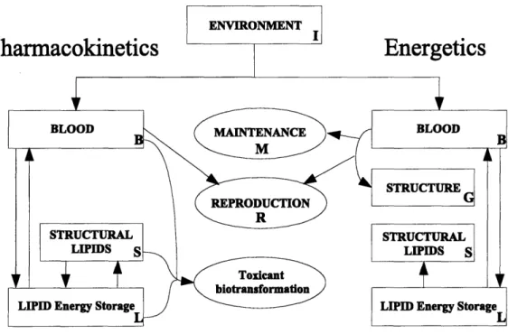
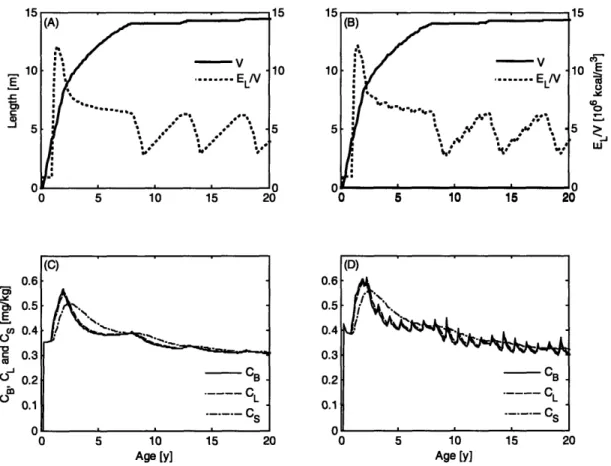
An individual acquires energy needed for its maintenance, growth, and reproduction from the environment. With that energy, the organism acquires toxicants. Both the energy and toxicants are distributed throughout the body. We keep track of these distributions by partitioning the organism into four compartments (Figure 2-1): blood (B), structure (G), structural lipids (S) and lipid energy storage (L). We summarize state variables and their units in 2.1. We summarize the dynamics of the model in Tables 2.2 and 2.3; in Table 2.4 we list the parameter values.
Pi
Figure 2-1: Model outline with pharmacokinetic (left) and energetic (right) model compartments. Reproduction (R), metabolism (M) and transformation of toxicants
act as sinks for energy, toxicants, or both. Toxicant biotransformation includes all
processes that change the molecular form of the modeled toxicant.
Table 2.1: Compartments and state variables with units. Compartment Energetics Toxicology
I Environment f Ci [mg/kg]
G Structure V[m3]
-B Blood EB [kcal] CB [mg/kg]
L Lipid energy storage EL[kcal] CL[mg/kg] S Structural Lipids Es[kcal] Cs[mg/kg]
R
Reproduction
--Table 2.2: Equations for the energy fluxes.
Flux [kcal/y] Description
FIB = Imaxf V2/3 intake of energy from the environment into blood
FBM = mV energy spent on maintenance
FBG = [GEB - FBM]+ energy utilized for growth
FBL = LEB energy flux from the blood to the lipid storage
FLB = /LkLEL energy flux from the lipid storage to the blood
FLS = es dv lipids transformed into structural lipids
FBR = (FBM + FBGR + FBR) flux of energy to reproduction (details in text)
k[X]+ is a shorthand notation for max(O, X).
1[X]+ is a shorthand notation for max(O, X).
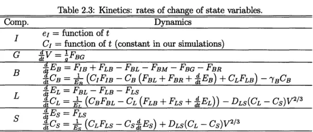
Table 2.3: Kinetics: rates of change of state variables.
Comp. Dynamics
I e = function of t
C = function of t (constant in our simulations)
G dtV = FBG
EB =FIB + FLB -FBL -FBM -FBG-FBR
B
dj~~~~~~~~
B
t-CB
d.
=1
(CIFIB - CB (FBL + FBR + EB) + CLFLB)d
- YBCBL
1EL = FBL- FLB - FLS
t CL = E,(CBFBL - CL (FLB + FLS + EL)) - DLS(CL - Cs)V2/ dTd
ES = FLS
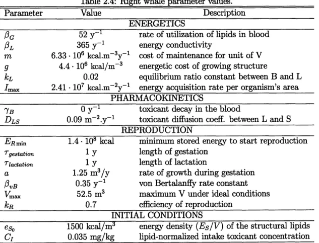
Table 2.4: Right whale parameter values.
Parameter Value Description
ENERGETICS
OG ~ 52 y-1 rate of utilization of lipids in blood
fL 365 y-1 energy conductivity
m 6.33 106 kcal.m-3y- 1 cost of maintenance for unit of V
g 4.4. 106 kcal/m-3 energetic cost of growing structure
kL 0.02 equilibrium ratio constant between B and L
Imax 2.41 107 kcal.m-2y-1 energy acquisition rate per organism's area
PHARMACOKINETICS
YB 0 y-1 toxicant decay in the blood
DLS 0.09 m-2.y - 1 toxicant diffusion coeff. between L and S
REPRODUCTION
ERmin 1.4. 108 kcal minimum stored energy to start reproduction
Tgestation 1 y length of gestation
lactation 1 y length of lactation
a 1.25 m3/y rate of growth during gestation
IvB 0.35 y-1 von Bertalanffy rate constant
Vm 52.5 m3 maximum V under ideal conditions
kR 0.7 efficiency of reproduction
INITIAL CONDITIONS
eso 1500 kcal/m3 energy density (Es/V) of the structural lipids
2.3.1 Energetics
We assume that all tissue may be characterized as either "energy reserves" or "struc-ture" (Kooijman 2000). The energy reserves are materials that can be utilized as an energy source for maintenance and growth (e.g. non-structural lipids, carbohydrates, and proteins). Any tissue the animal cannot utilize for energy during starvation (e.g. bones, structural lipids etc.) composes the structure. The exact composition of the
energy reserves and the structure depend on the species. Some tissues, such as muscle,
belong to both energy and structure to some degree: an organism uses muscle protein as energy when starving, but retains some even when it faces death from hunger.
We propose that the energy dynamics of a marine mammal can be captured by
focusing on lipid dynamics, as long as the relative amounts of different compounds
composing the energy reserves have a constant ratio. For example, muscle protein is depleted in a constant proportion to energy reserves in the blubber during starvation (Struntz et al. 2004 pp 18, Nordoy and Blix 1985). Hence, the dynamics of any component of reserves contains information about other types. We have chosen to keep track of lipids because they are the largest energy reserve in marine mammals, and because lipid dynamics determine the pharmacokinetics of lipophilic toxicants. The proportionality assumption does not hold for some types of energy reserves, e.g. protein and glycogen. This, however, does not influence overall energy dynamics because such types comprise only a small fraction of standing energy reserves; for example, during starvation 94% of energy consumption in grey seals (Halichoerus
grypus) comes from subcutaneous blubber (Nordoy and Blix 1985).
Lipids, and the tissues that hold them, have multiple functions (Struntz et al. 2004, Koopman et al. 2002). The largest pool of lipids is the blubber, but not all lipids in the blubber are readily metabolized. Lipids in the superficial blubber, i.e. lipids in and beneath the epidermal layer are barely metabolically active and can be neglected as a source of energy for the organism (Struntz et al. 2004). The metabolic activity of the blubber increases with depth, and deepest layers are most
metabolically active (Koopman et al. 2002, Aguilar and Borrell 1990). Recognizing this, we lump all metabolically inert lipids, such as those in the superficial blubber, into the "structural lipids" compartment (S), and all metabolically active lipids, such as those in the middle and deep layers of the blubber, into the "lipid energy storage"
compartment (L).
The structure compartment (G) includes all the structure except the structural lipids, and we assume that its composition remains constant through ontogeny. We further assume isomorphic growth, with the implication that the structural volume (V) of the animal is proportional to the cube of some measure of its length. We use V as the state variable representing structure. The blood (B) mediates all transfor-mations of energy and toxicants on short time scales, such as those in the gut and in the liver.
The dynamics of the energetics model is determined by fluxes (rates of flow of energy) between compartments. We denote a flux from compartment X into com-partment Y with Fxy.
Growth (FBG) and maintenance (FBM) of structure G
We assume the energy flux to growth and maintenance is proportional to the lipids available in the blood (EB), with a constant of proportionality that characterizes the rate of utilization of lipids, 8G- Maintenance has priority; an organism can utilize energy for growth only after it meets the energy requirement for maintenance.
The energy costs of maintenance depend on the size of the organism, and its energy expenditures for foraging and migration. We follow the dynamic energy budget (DEB) theory of Kooijman (2000) and assume that these costs are proportional to the volume of the organism. Hence, the energy flux FBM required for maintenance of an organism
of volume V is
FBM = mV, (2.1)
The flux of energy to growth, FBG, is the flux possible after maintenance has been met:
FBG = [GEB - FBM]+, (2.2)
where [x]+ is a short-hand notation for max(x, 0). If the energetic cost of growth by a unit of volume is g, the rate of growth of the organism is:
d V FBG (2.3)
dt g
Energy assimilation (FIB)
Only a fraction of the energy intake is assimilated and transported by the blood throughout the body. Hence, the flux of energy from the environment to the blood
(FIB) depends on food density in the environment, the organism's foraging ability, its
ability to process food, and its energy assimilation efficiency. We assume isomorphic growth, so that the energy intake from the environment is proportional to the area of the feeding structures (e.g. surface of the baleen), which is proportional to the surface area of the organism. Then,
FIB = ImaxfV2/3,
(2.4)
where Ira is the maximum assimilation rate per unit area, and f a saturating, Type II function of ej, the environmental energy density:
_
e~~~~~~~~~
~~(2.5)f = k +
el
(25)
where k, is the half-saturation constant. Throughout the paper, we refer to f as en-ergy availability. Since every organism has different food types and foraging patterns, the exact meaning of these parameters needs to be determined separately for each organism (see Gurney and Nisbet 1998, pp. 87 for details).
The energy intake determines the ultimate size of the organism, VO, and the maximum size of the organism, Vma,. At Vo, in a hypothetical constant environment and when not diverting energy into reproduction, the organism spends all the acquired energy on maintenance, i.e. FIB = FBM. From (2.1) and (2.4),
V.a (Ma). (2.6)
The maximum size is attained for f = 1:
Vm= (I- . (2.7)
Dynamic equilibrium between blood and lipid energy storage (FBL and
FLB)
The blood and lipid energy reserves are in direct contact and, therefore, try to
equi-librate through exchange of lipids. We assume the flux from one compartment into
another depends linearly on the amount of lipids in the origin compartment, and does not depend on anything in the destination compartment. Then, the flux of lipids from
B to L (FBL) and L to B (FLB) are:
FBL = LEB and (2.8)
FLB
= LkLEL.(2.9)
The net transport of lipids is equal to the difference between the two fluxes.
Growth of structural lipids S (FLs)
Growth is the only process relevant to structural lipids, and it is proportional to the growth of structure:
d Es= Es d V.
(2.10)
The biggest pool of structural lipids - the external blubber stratum - is not metabol-ically active, and does not differ significantly in composition between demographic groups (Aguilar and Borrell 1990). This holds for acoustic fats as well. Structural lipids are typically not significantly vascularized and are, therefore, not metabolically active. This leads us to assume that structural lipids are made from energy storage lipids directly by gradual processes such as de-vascularization, rather than through blood. Hence, the only flux to the compartment S is the flux from L:
dt
FLS = eso dV (2.11)
where eso is the proportion of lipids in the structure of the organism.
Reproduction (FBR)
After conception, mammalian reproduction has two parts: gestation and lactation. We model them separately because they have different modes of energy and toxi-cant transfers. In gestation, the mother transfers energy and toxitoxi-cants through the placenta. During lactation, the mother transfers energy and toxicants through milk. We assume that females conceive if, during the reproductive season, the energy in their lipid energy storage is greater than a certain critical value, ER. This assumption is consistent with the observed low variation of lipid storage energy density in female fin whales (Aguilar and Borrell 1990), suggesting that they reproduce upon reaching a certain 'trigger' lipid storage energy density. Whether female fin whales accumulate that energy after becoming pregnant, or become pregnant because they have reached the energy density is not clear. Nevertheless, given that onset of ovulation in some mammals depends on their energy reserves (Frisch et al. 1975, Van der Spuy 1985, Frisch 1990, but see Bronson and Manning 1991), that reproductive performance in mammals which experience seasonal food fluctuations depends on energy reserves of mature females (Frisch 1978, Gopalan and Naidu 1972, Lee 1987), and that fin
whale fecundity seems to be food-limited (Lockyer 1986), it is plausible to assume that marine mammals trigger ovulation depending on available energy storage. This
view is corroborated for right whales by observations (Angell 2005). We assume that
there are always enough males present that, upon ovulation, a female is fertilized and becomes pregnant.
The flux of energy to reproduction includes the flux needed for maintenance (FBmR), growth (FBR), and increase of energy reserves (FBER) of the young mammal during gestation and lactation:
FBR = k (FBR±+F+FR),
(2.12)
where kR is the reproductive efficiency of utilization of energy, potentially different
between gestation and lactation.
We assume that mother is able to meet all energetic needs of the calf during gesta-tion. We use an empirical model for fetal development commonly used for mammals (Martin and MacLarnon 1985), combined with the assumption that the mass of the fetus is proportional to its volume. According to the model, the volume of the fetus,
VF, at time r > 0.2Tgestation since conception is
VF(T) = a(r - 0.2rgestation )3. (2.13)
The volume of the fetus and the rate of change of the volume determine the energy needs of the fetus and, therefore, the mother's energy flux to reproduction.
Total energy flux to reproduction during gestation for r > 0.2rgestation includes the flux for maintenance of the fetus,
growth of the fetus,
F'dr
(2.15)
FBR(r) = gdVF(7),
(2.15)
and energy transferred to the fetus to build its energy reserves. In our model, the fetus acquires lipid energy reserves throughout gestation even though during fetal development energy is directed mainly towards growth, and lipid energy reserves are developed in the late stages of fetal development (Struntz et al. 2004). Energetically, the timing is not an issue because there is no cost associated with storing reserves, and only total amounts of matter transferred. For the same reason, the timing does not affect estimates of toxicant transfer because the toxicant transfer mainly depends on the total amount of lipids transferred. It may not be a significant issue for estimating gestational exposure either, because the fetus does not experience major bioaccumu-lation during gestation (the concentration of toxicants in its blood equilibrates with the mother's).
When connecting the energetics of gestation to pharmacokinetics, we assume that there is no placental barrier to toxicant transfer, and therefore the calf's and the mother's concentration of the toxicant in the blood tend to equilibrate. The validity of this assumption is not vital to our model because the bulk of energy (and, therefore, toxicant) is transferred during lactation (Young 1976). However, if exposure during fetal development is of concern, a more detailed model of fetal development, including the transport of lipids and toxicants across the placenta, may be required.
We assume that energy in the blood of the fetus is just sufficient to provide the energy flux for maintenance, and that the energy in the lipid energy storage compartment is in a dynamic equilibrium with the lipids in the blood:
1
Fetus= (2.16)
EB 3-i1 BR)'2.6
Ee -
1
-
F.(2.17)
/
3LkLF
.
the structural blubber, for r > 0.2Tgestation, is the energy needed to increase energy pools of the fetus proportionally to the change in volume:
FBER = 1 + ) m + e)
d
VF(T). (2.18)After birth, a newborn depends exclusively on its mother's milk for energy un-til weaning (Thomas and Taber 1984). During nursing, there are two competing processes: what the nursling demands and what the mother can give. The energy transferred is equal to the lesser of the two after adjusting for the inefficiencies of milk production and nursing. We assume that the nursling has an "ideal energy demand" which would allow it to grow following the von Bertalanffy growth curve, VB(t), with its ultimate goal to reach the maximum volume observed for the species (Vma). The energy flux required to meet the target growth curve VvB(t) is the sum of energy fluxes needed for maintenance, growth and increasing energy reserves of the nursling:
FBR = mVvB(t), (2.19)
dig,
FR -- g~V~B(t), and (2.20)
FBR = (eBo + eLo + eso) dVB(t) (2.21)
Here we assume that the nursling tries to match the energy density of its mother at conception, eBO in the blood, and eL0 in the lipid storage compartment.
Using our model, we calculate the growth of the nursling from its actual energy assimilation, which is the minimum between the ideal energy demand and what the mother can provide. When the mother is not able to meet the ideal energy de-mand, the nursling receives less then ideal energy flux. If this flux combined with the nursling's energy reserves is not sufficient to meet the maintenance requirements of the nursling, the nursling dies.
2.3.2 Pharmacokinetics
Our pharmacokinetic model keeps track of lipid-normalized concentrations of toxi-cants in an individual (Table 2.1) by modeling the biotransformation and movement of lipophilic toxicants between compartments of the organism. Unless otherwise men-tioned, all concentrations are lipid-normalized, expressed in milligrams of toxicant per kilogram of lipid (mg/kg). Upon entering the blood, the toxicants can either be bio-transformed (e.g. hydroxylated (Borga et al. 2004)), or transported throughout the body.
With the exception of the compartment G (structure without structural lipids), compartments in the pharmacokinetic model correspond to those of the energetics model. The compartment G is not directly involved in the toxicant dynamics because it does not include any lipids.
Lipophilic toxicants are not completely free to diffuse between compartments, nor are they all covalently bound to the lipids. Therefore, the transport of toxicants between compartments is a mixture of passive transport where toxicants behave as if they were not bound at all to the lipids, and lipid-facilitated transport where toxicants behave as if they were covalently bound to the lipids. We model both modes of transport.
Facilitated transport is assumed to be completely controlled by the fluxes of en-ergy in the energetics model: the toxicant flux from one compartment to another is proportional to the concentration of the toxicant in the source compartment and the flux of lipids from the source to the destination compartment. We assume no barriers to facilitated toxicant transport between compartments.
Passive transport involves the diffusion of toxicants between compartments. Dif-fusion rate is proportional to the difference in concentrations of toxicants, and to the boundary area between the compartments (Crank 2004) which, in view of our assumptions of an isomorphic animal, is assumed proportional to V2/ 3. Therefore, the rate of change of concentration of toxicants in compartments X and Y due to
diffusion is:
d dC
-Cy
--
Cx
= Dxy (Cx - Cy) V2/3. (2.22)dt dt
Regardless of the method of transport, we assume the toxicants redistribute within compartments instantaneously, i.e. the concentration within any compartment is
uniform.
Although the model can account for biotransformation of toxicants in all com-partments (Figure 2-1), the rates of biotransformation in the blood compartment are higher than in other compartments (Boon 1992, Borga et al. 2004). Furthermore, the other compartments communicate with the blood on time-scales much shorter than rates of biotransformation in those compartments. Therefore, we can simplify the model by assuming that only the biotransformations of the toxicants in the blood (e.g. by liver, gut and vascular endothelia) are significant. We represent these bio-transformations as a sink of toxicants - when biotransformed, toxicants are lost from the model.
Aside from the dilution by growth (proportional to-Cx Ex for any
compart-ment X), the rate of change of toxicant concentration of any compartcompart-ment is deter-mined by its sources, sinks, and passive and/or facilitated exchange of toxicants with other compartments. We do not model feedback of contaminants on rate processes
(e.g. Leung et al. 1990a, Leung et al. 1990b), but such feedback could be
incor-porated if necessary. The environment is the original source of all the accumulated toxicants.
Because of our choices of units motivated by the literature, we need a conversion
factor 7 to connect fluxes of energy ([kcal/y]) to fluxes of lipids ([kg/y]). The factor
has units of kg lipid per kcal (kg/kcal). We do not need to know its value, as it cancels out in the equations for rates of change of toxicant concentrations (Table 2.3).
Blood compartment (B)
We assume that toxicants in the blood experience both facilitated and passive trans-port to and from lipid energy storage. Fluxes of lipids to and from the blood com-partment are both large, even when the standing stock (EB, CB) is small. Because
of this, we assume that the dominant mode of transport of toxicants between the blood and the lipids is facilitated and ignore passive toxicant transport in and out of the blood compartment. Facilitated transports include the environmental input
(71CIFIB), the exchange with the lipid energy storage ( (CLFLB- CBFBL)) and a
sink: reproduction (-T)CBFBR).
Additional sinks include biotransformation (-7BCB), urinary excretion, and res-piratory exchange. Urine is not rich in lipids and, according to our assumptions, cannot be a large sink for non-metabolized lipophilic toxicants. Breathing is poten-tially both a source and a sink; we assume, however, that the respiratory exchange of lipophilic toxicants is much smaller than the nutritional input and can, therefore, be ignored. Hence, we ignore urinary excretion and respiratory exchange because we deem them not important, cannot parameterize them reliably, and account for them (at least partially) through biotransformation. These processes can be included in the model at a later date if necessary. Note that fecal excretion is accounted for by the assimilation efficiency (which is equal to the assimilation efficiency of energy): some lipids pass through the digestive system, and so do the toxicants associated with them.
Lipid energy storage (L)
Facilitated transport includes transfers between the lipid energy storage and the blood
(7 (CBFBL - CLFLB)) and a sink from the toxicant flux associated with the growth of the structural lipids (-T7CLFLs) . Passive transport consists of the diffusion between the two types of lipids (-DLS(CL - Cs)V23).


![[PDF] Formation approfondie sur les mathématiques et le langage Python | Cours informatique](data:image/gif;base64,R0lGODlhAQABAIAAAP///wAAACH5BAEAAAAALAAAAAABAAEAAAICRAEAOw==)