HAL Id: insu-01534692
https://hal-insu.archives-ouvertes.fr/insu-01534692
Submitted on 8 Jun 2017
HAL is a multi-disciplinary open access
archive for the deposit and dissemination of
sci-entific research documents, whether they are
pub-lished or not. The documents may come from
teaching and research institutions in France or
abroad, or from public or private research centers.
L’archive ouverte pluridisciplinaire HAL, est
destinée au dépôt et à la diffusion de documents
scientifiques de niveau recherche, publiés ou non,
émanant des établissements d’enseignement et de
recherche français ou étrangers, des laboratoires
publics ou privés.
Neutrally buoyant tracers in hydrogeophysics: Field
demonstration in fractured rock
Alexis Shakas, Niklas Linde, Ludovic Baron, John Selker, Marie-Françoise
Gerard, Nicolas Lavenant, Olivier Bour, Tanguy Le Borgne
To cite this version:
Alexis Shakas, Niklas Linde, Ludovic Baron, John Selker, Marie-Françoise Gerard, et al.. Neutrally
buoyant tracers in hydrogeophysics: Field demonstration in fractured rock. Geophysical Research
Letters, American Geophysical Union, 2017, 44 (8), pp.3663-3671. �10.1002/2017GL073368�.
�insu-01534692�
Neutrally buoyant tracers in hydrogeophysics:
Field demonstration in fractured rock
Alexis Shakas1 , Niklas Linde1 , Ludovic Baron1, John Selker2, Marie-Françoise Gerard3,
Nicolas Lavenant3, Olivier Bour3, and Tanguy Le Borgne3
1Applied and Environmental Geophysics Group, Institute of Earth Sciences, University of Lausanne, Lausanne, Switzerland, 2Department of Biological and Ecological Engineering, Oregon State University, Corvallis, Oregon, USA,3Géosciences
Rennes, Université de Rennes 1, CNRS, UMR 6118, Rennes, France
Abstract
Electrical and electromagnetic methods are extensively used to map electrically conductive tracers within hydrogeologic systems. Often, the tracers used consist of dissolved salt in water, leading to a denser mixture than the ambient formation water. Density effects are often ignored and rarely modeled but can dramatically affect transport behavior and introduce dynamics that are unrepresentative of the response obtained with classical tracers (e.g., uranine). We introduce a neutrally buoyant tracer consisting of a mixture of salt, water, and ethanol and monitor its movement during push-pull experiments in a fractured rock aquifer using ground-penetrating radar. Our results indicate a largely reversible transport process and agree with uranine-based push-pull experiments at the site, which is in contrast to results obtained using dense saline tracers. We argue that a shift toward neutrally buoyant tracers in both porous and fractured media would advance hydrogeophysical research and enhance its utility in hydrogeology.Plain Language Summary
Geophysical techniques allow for nondestructive monitoring of groundwater processes provided that contrasts in physical properties are available through time and space. To achieve this contrast, the common approach is to inject saline water (a so-called saline tracer) into the ground and to subsequently monitor its movement using geophysical measurements. Unfortunately, classical saline tracers are denser (thus heavier) than fresh groundwater, which leads to instabilities and downward movement of the tracer. This implies that the information gained from saline tracer tests might be unrepresentative of natural groundwater conditions. We introduce a saline tracer that has the same density as the ambient groundwater by mixing the saline tracer with ethanol. This enables, for the first time, geophysical imaging of groundwater flow and transport without associated density effects. By considering experiments performed in fractured rock, we demonstrate (1) that previously used dense saline tracers used for geophysical monitoring lead to very strong density effects, (2) that the new tracer solution can be imaged very well using geophysical techniques, and (3) that the recovered tracers (the so-called breakthrough curves) agree well with traditional tracer tests and hydrogeological theory.1. Introduction
Geophysics enables remote monitoring and imaging of subsurface mass transfer at scales ranging from decimeters [e.g., Garré et al., 2011; Beff et al., 2013], to meters [e.g., Slater and Sandberg, 2000; Singha and
Gorelick, 2005], kilometers [e.g., Falgàs et al., 2009; Rosas-Carbajal et al., 2015], and beyond [e.g., Zhdanov et al., 2011]. The need for methodological developments that ensure appropriate integration of geophysical
data in subsurface hydrology have given rise to the research field of hydrogeophysics [Hubbard and Linde, 2011; Binley et al., 2015], which has had an impact on hydrology over the last decade [National Research
Council, 2012]. In hydrogeophysics, geophysical experiments are made to support hydrological research and
applications. This implies not only that geophysical data should be informative of the processes being stud-ied but also that its acquisition should not perturb hydrological data or significantly affect the design of hydrological experiments.
In order to image a tracer (or contaminant plumes) with geophysics, there must exist a naturally occurring or imposed contrast in physical properties between the tracer (contaminant) and the surrounding forma-tion water. When such a contrast is present, geophysical imaging can provide insight into the transport
RESEARCH LETTER
10.1002/2017GL073368 Key Points:
• First geophysical monitoring of a neutrally buoyant and electrically conductive tracer
• Comparisons between neutrally buoyant and dense tracers highlight very different dynamics
• Neutrally buoyant tracers make geophysical monitoring experiments compatible with hydrogeological tracer tests
Correspondence to:
A. Shakas, [email protected]
Citation:
Shakas, A., N. Linde, L. Baron, J. Selker, M.-F. Gerard, N. Lavenant, O. Bour, and T. Le Borgne (2017), Neutrally buoyant tracers in hydrogeophysics: Field demon-stration in fractured rock, Geophys.
Res. Lett., 44, 3663–3671,
doi:10.1002/2017GL073368.
Received 7 MAR 2017 Accepted 10 APR 2017
Accepted article online 17 APR 2017 Published online 30 APR 2017
©2017. American Geophysical Union. All Rights Reserved.
Geophysical Research Letters
10.1002/2017GL073368
processes that take place in the hydrogeological system. In situ imaging of transport processes with geo-physics may thus help to unravel complex processes, such as anomalous transport, dual-domain mass transfer, or reversible/irreversible dispersion, that are often difficult to infer from breakthrough curve analysis alone [Swanson et al., 2012, 2015]. In groundwater geophysics, the contrast agent for tracer tests is often dissolved table salt (NaCl) [Day-Lewis et al., 2003; Singha and Gorelick, 2005; Doetsch et al., 2012; Shakas et al., 2016]. Salt increases the electrical conductivity and enables tracking of tracer plumes using electrical [Kemna et al., 2002; Singha and Gorelick, 2005], induction-based electromagnetic [e.g., Falgàs et al., 2009; Rosas-Carbajal
et al., 2015], or high-frequency electromagnetic [Day-Lewis et al., 2003; Tsoflias and Becker, 2008] methods.
Note that the studies mentioned above have been conducted in both fractured and porous-media systems. The salinity contrast needed for reliable geophysical imaging implies that the saline solution is significantly denser than the surrounding water, which results in buoyancy-induced tracer movement; this has been veri-fied in both laboratory experiments [e.g., Istok and Humphrey, 1995] and numerical tests [e.g., Beinhorn et al., 2005; Kemna et al., 2002]. Doetsch et al. [2012] provide a field demonstration of density effects using time-lapse electrical resistivity tomography. In accordance with numerical modeling, they found that a tracer injected in a gravel aquifer rapidly plunged to the underlying clay aquitard. Previous field experiments with lower salinity constrasts (and less density effects) at the site did not enable reliable time-lapse inversion results.
In the hydrogeophysics literature, it is rare to find field-based studies in which density effects are assessed or accounted for [e.g., Doetsch et al., 2012; Shakas et al., 2016; Haaken et al., 2016]. Even if density effects are considered in the modeling and associated inversion, the ubiquitous use of dense saline tracers in hydro-geophysics is problematic as they change the system dynamics [Tenchine and Gouze, 2005]. That is, the use of geophysics imposes constraints on experimental design that might be unacceptable for field hydrogeolo-gists. This implies (1) that hydrogeologists might be reluctant to consider geophysics in their work if they feel that hydrological experiments will be compromised by using dense tracers, (2) that comparisons between hydrogeophysical results and hydrogeological experiments using nonsalt tracers are difficult, and (3) that the inferred system properties and hydrological processes might have low predictive capacity in describing natural flow dynamics.
In this work, we introduce a neutrally buoyant tracer based on a water-salt-ethanol mixture that we refer to as wethanalt. Ethanol is fully miscible and has a similar viscosity as water. It is less dense than water and can be used to ensure that the resulting tracer solution is neutrally buoyant, while it maintains a high electrical conductivity with respect to the formation water. Furthermore, ethanol has the distinct advantage of being nontoxic [Thakker, 1998] and biodegradable [Schaefer et al., 2010].
We present two field experiments in which we demonstrate the value of using neutrally buoyant and electrically conductive tracers for imaging transport processes. We consider push-pull experiments at a well-characterized fractured rock site with geophysical monitoring using single-hole ground-penetrating radar [Dorn et al., 2011, 2012]. Our results are compared with previous experiments at the site that were carried out using dense saline solutions [Shakas et al., 2016] and a traditional push-pull experiment using a fluorescein tracer, without geophysical monitoring [Kang et al., 2015].
2. Methodology
The properties of ethanol-water and salt-water mixtures have been tabulated [Haynes, 2016]. To the best of our knowledge, such a laboratory study does not exist for wethanalt (ethanol-water-salt mixtures). Here we present a practical method for obtaining a neutrally buoyant wethanalt mixture by utilizing the existing tables as a guide and further fine-tuning the density in the field. In the following section, where not otherwise noted, the material properties of ethanol, water, and salt are taken from Haynes [2016].
2.1. Wethanalt Properties
Ethanol (C2H6O) has a density of 0.789 g cm−3, relative electrical permittivity of 25.3 (zero-frequency limit), and
dynamic viscosity of 1.203 mPa s at 20∘C. At the same temperature, demineralized water (H2O) has a density of 1 g cm−3, relative electrical permittivity of 81 and dynamic viscosity of 1.004 mPa s. Both liquids are electrically
resistive, and it is the addition of salt to the mixture that will determine the electrical conductivity. The most common choice of salt in hydrogeophysical applications is sodium chloride (NaCl), that dissociates into Na+
Ethanol and water are miscible in all proportions, and their mixing results in an exothermic reaction [Peeters
and Huyskens, 1993] which leads to an increase in temperature when the mixture is prepared. Another
prop-erty of ethanol-water mixtures is that the dynamic viscosity of the mixture is increased compared with the constituents. The maximum viscosity of the mixture is 2.85 mPa s (20∘C) when the mass proportion of ethanol to water is 0.42:0.58. Ethanol does not pose any health risks when diluted with water [Thakker, 1998] and is biodegradable [Schaefer et al., 2010], which implies that it may increase microbial activity when used as a tracer.
2.2. Wethanalt Preparation
The preparation of a neutrally buoyant wethanalt solution is complicated by the facts (1) that the density of an ethanol-water mixture does not average arithmetically when adding salt and (2) that the necessary preci-sion in density needs to be sufficiently low (for instance, Istok and Humphrey [1995] perform a laboratory study and report density effects for density variations (Δ𝜌) in the range 0.0075% ≤ Δ𝜌 ≤ 0.15%). To achieve this, our preferred field procedure is to first rely on tabulated values in Haynes [2016] to obtain a desired density of an initial ethanol-water mixture and then assume arithmetic averaging to predict the necessary amount of salt to add in order for the density to be equal to that of the formation water. We then prepare a wethanalt mixture with 5% less salt than predicted with this simple model. For our experiments we first mixed 85 L of demineralized water with 25 L of (99.98%) ethanol; this resulted in an increase in temperature of 8∘C. The vis-cosity of the mixture was 2.26 mPa s according to Haynes [2016]. We then pumped formation water through a plastic tube that was coiled in the ethanol-water container, in order to reduce the temperature of the mix-ture to the ambient water temperamix-ture. Using this approach, we successfully reduced the temperamix-ture of the tracer mixture in all wethanalt experiments from ∼ 24∘C to ∼ 18∘C, while the ambient water temperature is 16∘C.
To achieve a neutrally buoyant solution, we relied on Archimedes’ principle, namely, that “Any object, wholly or partially immersed in a fluid, is buoyed up by a force equal to the weight of the fluid displaced by the object” [Archimedes (250 BC), 1897]. To do so, we used two containers: the first filled with the wethanalt mix-ture and the second containing formation water. In the second container, we submerged a balloon that we carefully filled with formation water and allowed for any air bubbles to escape. The balloon weighed 3.5 kg and was slightly positively buoyant, so we further adjusted its weight with plastic O rings (3 g each with a density of 1.1 g cm−3, resulting in a net submerged weight of 0.3 g per O ring) until we reached neutral
buoyancy (i.e., not observing any vertical movement of the balloon when suspended in the middle of the water-filled container). The weight adjustments were made to a precision below 0.1 g kg−1. We then
trans-ferred the balloon with the attached O rings to the wethanalt container, in which we had mixed an initial amount (4 kg) of salt in the ethanol-water mixture, well below the amount (4.22 kg) predicted from arith-metic averaging. We then proceeded to add salt in increments between 20 and 80 g, until the balloon was neutrally buoyant in the wethanalt mixture. In the final stage, a total of 4.44 kg of salt was added and the mix-ture was stirred with a mixing propeller to ensure well-mixed conditions. This procedure allows us to obtain a wethanalt solution that is at most 0.01% different in density than the formation water. While ethanol is biodegradable [Schaefer et al., 2010], it also does not pose any substantial health risks after sufficient dilution [Thakker, 1998].
2.3. Setup of the Field Experiment
We performed the wethanalt push-pull experiments in a well-characterized fractured granitic aquifer located in Brittany, France (http://hplus.ore.fr/en). Previous studies indicate that flow at the site is dominated by a few, highly transmissive fractures [Le Borgne et al., 2007; Dorn et al., 2011]. All the experiments were performed in two adjacent boreholes, B1 and B2, that are separated by ∼ 6 m. A double-packer system isolated a fracture intersecting the B1 borehole at 77.8 m, in which we injected the tracer followed by an almost equal volume of formation water (chaser). We then reversed the flow in order to retrieve the tracer, either immediately (push-pull) or after a waiting period (push-wait-pull) during which the pumps were off.
Ground-penetrating radar (GPR) monitoring took place at 5 cm intervals between 60 m and 85 m depth along borehole B2, which was isolated with a borehole liner [Shakas et al., 2016]. In an effort to further separate the direct wave from the reflections of interest, we reduced the transmitter-receiver offset from 4 m by Shakas
Geophysical Research Letters
10.1002/2017GL073368
2.4. Data Processing
2.4.1. Tracer Breakthrough Curves
We transformed electrical conductivity values, measured using a conductivity-temperature-depth (CTD) diver located at the outlet of the pump used for pulling, into salt concentration [Sen and Goode, 1992]. We then removed the background concentration and normalized the data to the injected tracer concentration, also with the background concentration removed. We also shifted the breakthrough data to account for the time it takes for the water to flow through the tubing from the packer to the outflow location. The experiments using the dense saline tracer published by Shakas et al. [2016] were performed in 2014 and the wethanalt experiments in 2016. For both field campaigns, we performed a series of tracer experiments. This implies that any unrecovered salt may lead to an increasing background concentration over time. To account for this, we present the uncertainty in the breakthrough curves (BTCs) with a thickness (see Figures 1i, 2i, and 3) obtained by varying the considered background concentration between a minimum (ambient concentration at the beginning of the field campaign) and a maximum (initial concentration at the beginning of each experiment). In order to compare experiments with different tracer/chaser volumes and flow rates, we normalize the time of each experiment with the theoretical peak arrival time. In an ideal push-pull experiment [Neretnieks, 2007], the theoretical peak arrival time (tpeak) measured from the onset of pulling depends on the duration of both
injection (tinjection) and chasing (tchasing) and is given by tpeak = tinjection∕2 + tchasing. The same formula applies
to push-wait-pull experiments in the absence of ambient flow. 2.4.2. Migrated GPR Difference Sections
The processing of the GPR data is described in Shakas et al. [2016]. To each GPR trace, we apply a bandpass filter with a frequency window between 20 and 200 MHz (the emitted signal is centered at 100 MHz) followed by minor time shifts to align collocated traces. Compared with Shakas et al. [2016], the only difference in the processing was the use of singular value decomposition (SVD) to remove the direct wave. We accomplish this by decomposing each GPR section that we then reconstruct without the first singular value, which cor-responds mainly to the direct wave. We then take the difference of each section and the reference (taken before the initiation of the push-pull experiment), apply a time gain, and finally use a Kirchhoff migration algo-rithm with a constant velocity model of𝑣 = 0.12nsm. This results in migrated GPR difference sections where the presence of the conductive tracer manifests itself as alternating (green-orange) stripes, whose horizontal extent is caused by the finite size of the source wavelet [Shakas et al., 2016]. For visualization purposes, we suppress any reflections that are below the estimated noise level of our GPR data set (computed as 15% of the maximum amplitude).
3. Results
We now compare the BTCs and the migrated GPR difference sections obtained from the combined experi-ments with a saline tracer and wethanalt. Here we consider both push-pull and push-wait-pull setups. For the BTCs, we use a normalized time,𝜏 = t∕tpeak, where t corresponds to the time after the onset of pulling and tpeak
is the theoretical peak arrival time. We also use a normalized concentration, c = C∕C0that corresponds to the
measured concentration (C) divided by the initial tracer concentration (C0), after removing the background
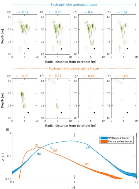
concentration from both. It takes about 3 min to acquire GPR data over the considered depth range, so each GPR section is indicated by an approximate time. The main experimental parameters are listed in Table 1. A comparison between the push-pull experiments is made in Figure 1, where all time references are made (in normalized time) to the onset of the pulling phase. Figure 1 displays representative migrated GPR differ-ence sections for the wethanalt (Figures 1a–1d) and saline (Figures 1e–1h) push-pull experiments, and the BTCs are plotted in Figure 1i. At the onset of pulling, the wethanalt tracer (Figure 1a) is localized within a depth range of 67 m to 72 m, while the saline tracer (Figure 1e) is found within 69 m to 76 m. At𝜏 close to 0.25, the wethanalt tracer (Figure 1b) is found over the same depth range while the dense saline tracer (Figure 1f ) has quickly migrated down toward the injection location. These results are in accordance with the peaks of the BTCs that occur with𝜏 = 0.9 and c = 0.45 for wethanalt, while 𝜏 = 0.27 and c = 0.23 for the dense saline tracer. This indicates that the measured peak arrival is close to the theoretical peak when using wethanalt, while it is much smaller when using a dense saline tracer. Shakas et al. [2016] demonstrated through modeling that this early peak arrival of the dense saline tracer was a consequence of density effects and the geometry of the fracture network. Reflections from the wethanalt tracer remain visible, from 67 m to 77 m, at much later times (Figure 1d) than the peak arrival measured in the borehole.
Figure 1. Results from two separate push-pull experiments using either wethanalt or a dense saline tracer (experiments a and c in Table 1, respectively). The migrated GPR difference sections for (a–d) wethanalt and (e–h) dense saline tracers are presented at similar normalized acquisition times (𝜏), where the black circle corresponds to the tracer injection location. The corresponding breakthrough curves are plotted in logarithmic scale (i) as a function of normalized time and normalized concentration (c). The resulting uncertainty due to the background salt concentration is indicated by the thickness of each curve.
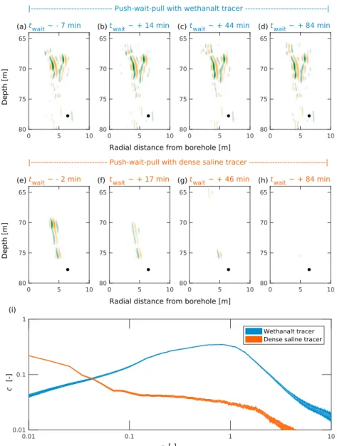
The push-wait-pull experiments are presented in Figure 2. All migrated GPR difference sections shown were acquired during the waiting time, so their acquisition times are referenced in minutes from the onset of wait-ing (twait). After the pushing phase (Figures 2a and 2e), the distribution of both tracers is similar to the push-pull
experiment (cf. Figures 1a and 1e), thereby indicating a strong reproducibility of the experiments. After 17 min, the saline tracer has sunk considerably (Figure 2f ) due to its high density and is thereafter hardly detectable (Figures 2g and 2h). On the contrary, the migrated GPR difference sections for the wethanalt tracer remain almost identical during the whole waiting time (Figures 2a–2d). Once more, the peak arrivals of the BTCs sup-port these observations with𝜏 = 0.83 and c = 0.35 for wethanalt, while 𝜏 = 0.008 and c = 0.05 for the dense saline tracer. Again, the peak arrival of the dense tracer occurs much earlier than predicted from the theoreti-cal peak arrival time. Later GPR difference sections (not shown) confirm that the wethanalt tracer is still visible in the migrated GPR difference sections at times twice as long as the theoretical peak arrival.
Geophysical Research Letters
10.1002/2017GL073368
Figure 2. Results from two separate push-wait-pull experiments using either wethanalt or a dense saline tracer (experiments b and d in Table 1, respectively). The migrated GPR difference sections for (a–d) wethanalt and (e–h) dense saline tracers are presented at similar acquisition times referenced from the waiting phase (twait), where the black circle corresponds to the tracer injection location. The corresponding breakthrough curves are plotted in logarithmic scale (i) as a function of normalized concentration (c) and normalized time (𝜏) since the initiation of pulling. The resulting uncertainty due to the background salt concentration is indicated by the thickness of each curve.
4. Discussion
The migrated GPR difference sections of the two push-pull experiments (Figure 1) suggest that different spatial regions of the fractured system are probed when using a neutrally buoyant or a dense saline tracer. The saline tracer remains closer to the injection location and is not pushed much further by chasing. This is expected since we are trying to displace a dense tracer with lighter formation water. Moreover, it is also in accordance with flow and transport simulations [Shakas et al., 2016; Haaken et al., 2016]. When wethanalt is used as a tracer, the chaser effectively pushes the tracer away from the injection location (Figure 1a) and into upper regions of the fractured system. By doing so, the migrated GPR difference sections from the wethanalt tracer probe an additional fracture that appears above 70 m depth and beyond 5 m radius (Figures 1a–1d). This fracture is not present in the migrated GPR difference sections acquired with the dense saline tracer (Figures 1e–1h).
Figure 3. Inferred impulse-response breakthrough curves for the wethanalt experiments (experiments a and b in Table 1) obtained by deconvolution. The uncertainty associated with the unknown background salinity is represented by the thickening of the lines at late times. For comparison purposes, we also plot the breakthrough curve from the push-pull experiment by Kang et al. [2015] described in Table 1.
In the push-wait-pull experiments (Figure 2), the impact of density is even more evident. While the tracer distri-bution after pushing is similar to their push-pull counterparts (compare Figures 1a with 2a and 1e with 2e), the dense saline tracer quickly migrates toward the injection location during the waiting period (Figures 2f–2h). On the contrary, the wethanalt tracer provides consistent, high-amplitude reflections throughout the waiting period (Figures 2a–2d), suggesting that the tracer distribution remains the same during this time. This indi-cates that the sinking observed when using a dense saline tracer is primarily due to density effects and not to ambient flow, as the ambient flow should also affect the wethanalt tracer. This finding is further supported by the similar peak arrival times of the wethanalt tracer in the push-pull and push-wait-pull configurations (𝜏 = 0.9 and 𝜏 = 0.83, respectively). Nevertheless, the waiting period allows for more diffusion of the wethanalt tracer and possibly some ambient flow effects that manifest as a decrease of the peak concentration in the BTC between the push-pull (c = 0.45) and push-wait-pull (c = 0.35) configurations.
To further assess the suitability of wethanalt as a neutrally buoyant tracer, we compare our BTCs with the push-pull BTC by Kang et al. [2015], performed at the same fracture location but with an almost instantaneous injection of a neutrally buoyant fluorescein tracer (see Table 1 for parameters). To remove the imprint of the injection period from the wethanalt BTCs, we model the push-pull experiment as the convolution of a lin-ear, time-invariant source operator with the impulse-response of the system. We infer the impulse-response using an iterative least squares inversion [Menke, 2012] with smoothness and positivity constraints [Cirpka
et al., 2007]. Convergence is reached when the positivity constraints stop changing. In order to compare the
late-time slope of the BTCs, we normalize concentration to the peak concentration and time to the peak arrival time and plot the BTCs in Figure 3. The push-pull experiment shows a late-time tailing comparable to the BTC from Kang et al. [2015], while the push-wait-pull experiment indicates a smaller slope. This indicates that the wethanalt BTCs are consistent with the fluorescein BTCs, in particular regarding the late-time concentration decay, which is important for investigating anomalous transport and dual-domain mass transfer processes.
Table 1. Experimental Parameters for (a) Push-Pull and (b) Pull With Wethanalt, (c) Push-Pull and (d) Push-Wait-Pull With a Saline Tracer, and (e) the Fluorescein-Based Push-Push-Wait-Pull Experiment by Kang et al. [2015]
Tracer Tracer Ethanol Tracer Density Chaser Waiting Pumping Mass ID Volume (L) Salinity (g kg−1) (%) (kg m−3) Volume (L) Time (min) Rate (L min−1) Recovery (%)
a 106 40 22.73 1000 113 0 2.9 92±3
b 106 40 22.73 1000 108 120 2.9 78±3
c 100 44 0 1044 90 0 3.3 71±9
d 100 42 0 1042 90 227 3.3 50±10
Geophysical Research Letters
10.1002/2017GL073368
5. Conclusions
Our results suggest that wethanalt, a mixture of saline water and ethanol, is a suitable tracer for conducting geophysical monitoring using electrical or electromagnetic methods, when density effects are undesir-able. Tracer test experiments conducted in push-pull and push-wait-pull configurations, in conjunction with single-hole GPR monitoring, confirm that wethanalt provides a strong GPR signal and does not exhibit the density-driven downward flow observed in our past experiments with dense saline tracers [Shakas et al., 2016]. Therefore, wethanalt may significantly improve our ability to monitor flow and transport processes in situ with hydrogeophysical methods, without the complications of density-driven flow and instabilities. Indeed, our results suggest that if a dense saline tracer is used, it is possible that observations (and inferences) made about the hydrogeological system are unrepresentative of the ambient conditions and may differ significantly if a neutrally buoyant tracer is used instead. We also propose a practical way to prepare a wethanalt mix-ture with a high electrical conductivity at ambient density for any freshwater hydrogeological application. Additionally, wethanalt is biodegradable, comparatively cheap to produce, and does not pose any health risks. We anticipate that wethanalt or other neutrally buoyant saline tracers will play an important role in advancing hydrogeophysics and in situ monitoring of transport processes. Moreover, since the buoyancy of wethanalt can be adjusted, wethanalt mixtures open a new window on the use of buoyant and nonbuoyant tracers for studying density effects.
References
Archimedes (250 BC) (1897), On Floating Bodies, Translation by H. T Little, p. 257, Cambridge Univ. Press, Cambridge.
Beff, L., T. Günther, B. Vandoorne, V. Couvreur, and M. Javaux (2013), Three-dimensional monitoring of soil water content in a maize field using electrical resistivity tomography, Hydrol. Earth Syst. Sci., 17(2), 595–609.
Beinhorn, M., P. Dietrich, and O. Kolditz (2005), 3-D numerical evaluation of density effects on tracer tests, J. Contam. Hydrol., 81(1), 89–105. Binley, A., S. S. Hubbard, J. A. Huisman, A. Revil, D. A. Robinson, K. Singha, and L. D. Slater (2015), The emergence of hydrogeophysics for
improved understanding of subsurface processes over multiple scales, Water Resour. Res., 51, 3837–3866, doi:10.1002/2015WR017016. Cirpka, O. A., M. N. Fienen, M. Hofer, E. Hoehn, A. Tessarini, R. Kipfer, and P. K. Kitanidis (2007), Analyzing bank filtration by deconvoluting
time series of electric conductivity, Groundwater, 45(3), 318–328, doi:10.1111/j.1745-6584.2006.00293.x.
Day-Lewis, F. D., J. W. Lane Jr., J. M. Harris, and S. M. Gorelick (2003), Time-lapse imaging of saline-tracer transport in fractured rock using difference-attenuation radar tomography, Water Resour. Res., 39(10), 1290, doi:10.1029/2002WR001722.
Doetsch, J., N. Linde, T. Vogt, A. Binley, and A. G. Green (2012), Imaging and quantifying salt-tracer transport in a riparian groundwater system by means of 3D ERT monitoring, Geophysics, 77(5), B207–B218, doi:10.1190/geo2012-0046.1.
Dorn, C., N. Linde, T. Le Borgne, O. Bour, and L. Baron (2011), Single-hole GPR reflection imaging of solute transport in a granitic aquifer,
Geophys. Res. Lett., 38, L08401, doi:10.1029/2011GL047152.
Dorn, C., N. Linde, J. Doetsch, T. Le Borgne, and O. Bour (2012), Fracture imaging within a granitic rock aquifer using multiple-offset single-hole and cross-hole GPR reflection data, J. Appl. Geophys., 78, 123–132, doi:10.1016/j.jappgeo.2011.01.010.
Falgàs, E., J. Ledo, A. Marcuello, and P. Queralt (2009), Monitoring freshwater-seawater interface dynamics with audiomagnetotelluric data,
Near Surf. Geophys., 7(5–6), 391–399.
Garré, S., M. Javaux, J. Vanderborght, and H. Vereecken (2011), Three-dimensional electrical resistivity tomography to monitor root zone water dynamics, Vadose Zone J., 10(1), 412–424, doi:10.2136/vzj2010.0079.
Haaken, K., G. P. Deidda, G. Cassiani, R. Deiana, M. Putti, C. Paniconi, C. Scudeler, and A. Kemna (2016), Flow dynamics in hyper-saline aquifers: Hydro-geophysical monitoring and modelling, Hydrol. Earth Syst. Sci., 21(3), 1439–1454, doi:10.5194/hess-2016-450. Haynes, W. M. (2016), CRC Handbook of Chemistry and Physics, 97th edn., CRC Press, Boca Raton, Fla.
Hubbard, S. S., and N. Linde (2011), Hydrogeophysics, in Treatise on Water Science, vol. 2 (Hydrology), edited by S. Uhlenbrook, chap. 2.15, pp. 402–434, Elsevier, Oxford, doi:10.1016/B978-0-444-53199-5.00043-9.
Istok, J. D., and M. D. Humphrey (1995), Laboratory investigation of buoyancy-induced flow (plume sinking) during two-well tracer tests,
Groundwater, 33, 597–604, doi:10.1111/j.1745-6584.1995.tb00315.x.
Kang, P. K., T. Le Borgne, M. Dentz, O. Bour, and R. Juanes (2015), Impact of velocity correlation and distribution on transport in fractured media: Field evidence and theoretical model, Water Resour. Res., 51, 940–959, doi:10.1002/2014WR015799.
Kemna, A., B. Kulessa, and H. Vereecken (2002), Imaging and characterisation of subsurface solute transport using electrical resistivity tomography (ERT) and equivalent transport models, J. Hydrol., 267(3), 125–146, doi:10.1016/S0022-1694(02)00145-2.
Le Borgne, T., O. Bour, M. S. Riley, P. Gouze, P. A. Pezard, A. Belghoul, and E. Isakov (2007), Comparison of alternative method-ologies for identifying and characterizing preferential flow paths in heterogeneous aquifers, J. Hydrol., 345(3), 134–148, doi:10.1016/j.jhydrol.2007.07.007.
Menke, W. (2012), Geophysical Data Analysis: Discrete Inverse Theory, vol. 45, Acad. Press, Waltham, Mass.
National Research Council (2012), Challenges and Opportunities in the Hydrologic Sciences, Natl. Acad. Press, Washington, D. C. Neretnieks, I. (2007), Single well injection withdrawal tests (SWIW) in fractured rock: Some aspects on interpretation, SKB Rep. R-07-54,
Dep. of Chem. Eng. and Technol., Royal Inst. of Technol., Stockholm, Sweden.
Peeters, D., and P. Huyskens (1993), Endothermicity or exothermicity of water/alcohol mixtures, J. Mol. Struct., 300, 539–550. Rosas-Carbajal, M., N. Linde, J. Peacock, F. I. Zyserman, T. Kalscheuer, and S. Thiel (2015), Probabilistic 3-D time-lapse inversion of
magnetotelluric data: Application to an enhanced geothermal system, Geophys. J. Int., 203(3), 1946–1960, doi:10.1093/gji/ggv406. Schaefer, E. C., X. Yang, O. Pelz, D. T. Tsao, S. H. Streger, and R. J. Steffan (2010), Anaerobic biodegradation of iso-butanol
and ethanol and their relative effects on BTEX biodegradation in aquifer materials, Chemosphere, 81(9), 1111–1117, doi:10.1016/j.chemosphere.2010.09.002.
Sen, P. N., and P. A. Goode (1992), Influence of temperature on electrical conductivity on shaly sands, Geophysics, 57(1), 89–96, doi:10.1190/1.1443191.
Acknowledgments
This research was supported by the Swiss National Science Foundation under grant 200021-146602, by the French National Observatory H+ (hplus.ore.fr/en), and by the ANR project CRITEXANR-11-EQPX-0011. Selkes’ participation in this work was supported by the U.S. National Science Foundation grant 1551483. We would like to thank Olivier Bochet and Christophe Petton for their indispensable help in the field, Peter Kang for providing the fluorescein push-pull data and two anonymous reviewers for their comments on the manuscript. The data and code required to reproduce the results are available from the first author upon request, and the tracer test data are available from the H+ database.
Shakas, A., N. Linde, L. Baron, O. Bochet, O. Bour, and T. Le Borgne (2016), Hydrogeophysical characterization of transport processes in fractured rock by combining push-pull and single-hole ground penetrating radar experiments, Water Resour. Res., 52, 938–953, doi:10.1002/2015WR017837.
Singha, K., and S. M. Gorelick (2005), Saline tracer visualized with three-dimensional electrical resistivity tomography: Field-scale spatial moment analysis, Water Resour. Res., 41, W05023, doi:10.1029/2004WR003460.
Slater, L. D., and S. K. Sandberg (2000), Resistivity and induced polarization monitoring of salt transport under natural hydraulic gradients,
Geophysics, 65(2), 408–420, doi:10.1190/1.1444735.
Swanson, R. D., K. Singha, F. D. Day-Lewis, A. Binley, K. Keating, and R. Haggerty (2012), Direct geoelectrical evidence of mass transfer at the laboratory scale, Water Resour. Res., 48, W10543, doi:10.1029/2012WR012431.
Swanson, R. D., A. Binley, K. Keating, S. France, G. Osterman, F. D. Day-Lewis, and K. Singha (2015), Anomalous solute transport in saturated porous media: Relating transport model parameters to electrical and nuclear magnetic resonance properties, Water Resour. Res., 51, 1264–1283, doi:10.1002/2014WR015284.
Tenchine, S., and P. Gouze (2005), Density contrast effects on tracer dispersion in variable aperture fractures, Adv. Water Res., 28(3), 273–289, doi:10.1016/j.advwatres.2004.10.009.
Thakker, K. D. (1998), An overview of health risks and benefits of alcohol consumption, Alcoholism Clin. Exp. Res., 22, 285–298, doi:10.1111/j.1530-0277.1998.tb04381.x.
Tsoflias, G. P., and M. W. Becker (2008), Ground-penetrating-radar response to fracture-fluid salinity: Why lower frequencies are favorable for resolving salinity changes, Geophysics, 73(5), J25–J30, doi:10.1190/1.2957893.
Zhdanov, M. S., R. B. Smith, A. Gribenko, M. Cuma, and M. Green (2011), Three-dimensional inversion of large-scale EarthScope magnetotelluric data based on the integral equation method: Geoelectrical imaging of the Yellowstone conductive mantle plume,