Design and analysis of robots that perform dynamic tasks using internal body motion

(1)

Design and Analysis of

Robots that Perform Dynamic Tasks

Using Internal Body Motion

by

Kevin Lawrence Brown

B.S.M.E., Massachusetts Institute of Technology

(1988)

M.S.M.E.,Massachusetts Institute of Technology (1990)

Submitted to the Department of Mechanical Engineering in partial fulfillment of the requirements for the degree of

DOCTOR OF PHILOSOPHY

at the

MASSACHUSETTS INSTITUTE OF TECHNOLOGY

September, 1994

The author hereby grants to MIT permission to reproduce and to distribute copies of this thesis document in whole or in part.

Signature of Author

Department of Mechanical Engineering July, 1994 Certified by

Haruhiko Asada Professor of Mechanical Engineering Thesis Supervisor Acceptea oy

Ain A. Sonin Chairman, Graduate Committee

LIBRARIES

(2)

Design and Analysis of Robots that Perfonn Dynamic Tasks

Using Internal Body Motion

by

Kevin Lawrence Brown

Submitted to the department of Mechanical Engineering on June 17, 1994, in partial fulfillment of the requirements for the degree of Doctor of Philosophy

A new approach to robot design and control specifically for dealing with heavy loads is presented in this thesis. Inspired by human dynamic motion, we explore dynamic task strategies to create large forces by dynamically moving the internal body. This technique can produce a much greater force than the traditional quasi-static technique. The strategy of this dynamic task performance is three-fold. One is to store a large momentum in the internal body motion and discharge the momentum at the interaction between the robot's end-effector and the environment. Second, the robot takes advantage of specific postures of the arm and leg to create a large mechanical advantage which allows for efficient load bearing and transmission of actuator torques to the end-effector. Third, peak outputs of robot actuators are utilized for short periods of time. These peak outputs can be up to an order-of-magnitude higher than their continuos rated torques.

The basic concept of this dynamic task strategy is described along with two exemplary case studies: dynamic lifting of a heavy weight and opening a stuck door. Kinematic and dynamic behavior of robots is analyzed. and conditions for the robot structure to perform such dynamic tasks are obtained. The dynamic trajectory of the internal body motion as well as one for the end effector motion are optimized by parametric representation of dynamic task performance. The performance index is based on the heat dissipated in the robot's motors. Initial parameter estimates for the optimization were derived from data measured of human motion. Simulation of the lifting task found that a robot designed with the appropriate motors and gear ratios requires 46% less dissipated energy using the dynamic method compared to a non-coordinated trajectory approach. A prototype robot is designed, built and tested. Experiments demonstrate the feasibility and effectiveness of the dynamic task strategies.

(3)

Acknowledgments

I would like to thank Prof. Asada, for if it were not for his zealous encouragement, his guidance and writing lessons, I would never have written anything like this thesis. I would also like to thank Dr. J. Ken Salisbury and Prof. Woody Flowers for their support and guidance as committee members.

I am grateful for the love, technical support, and understanding from my wonderful girlfriend Susanna Leveroni. If it were not for her help I would have never finished. I would like to tell my mother how much I appreciate her believing in me for my entire life and for always telling me that anything was possible. I would like to thank my brother Jeremy who I look up to more than anyone. He has always been there when I needed him with the most helpful support. I would like to thank Lee Cohn for being a support for my mother and for helping me through many years of my college. I would like to thank my father, the most brilliant man I know, for his guidance and for always having the answers to any question. I would like to thank Leigh for being the best thing that has ever happen to my father. In addition I would like to thank my brother Steven who has inspired me by his bravery.

I am very thankful to Hugh Herr and the people at the Concord Field Station for there help with the lift measurements. I very much appreciate Randy Pflueger and Dr. Luis Martins, for being subjects for the lift experiments. Their time and insight was critical to this thesis.

I appreciate the patience and support of my close friends, Edward Glicken, Daniel Sobek, Chistopher Scott Jones, Adam Simha, Gus Rancatore, Mark Lubratt, Lee Wienstien and Corine Bickley.

I would also like to thank, Edward Lanzilotta, Mark West, Dr. Jahng Park, Booho Yang, Dr. Sheng Liu, Sooyong Lee, Daniel Braunstein, Xiangdong He, Emile Chamas, Shih-hung Li, Nathan Delson, Nicholas Patrick, David Schloerb, Sudhendu Rai, Anton Pil,

(4)

Noriyuki Fujiwara, Samir Nafeh, Susan Ipri and everybody else in Prof Asada's lab for always answering my question with patience.

There are many others at MIT that have help me to finish this thesis over the years that I would like to thank: Eric Vaaler, Prof. William Durfee, Prof. Sheridan, Prof Amar Bose, Leaslie Regan, Sabina Rataj, Veronica Culbert, Joseph (Tiny) Caloggerio, Norm Mac Askill and Bob Nuttal.

I would also like to thank two outstanding professors that I had at Eastern Illinois University: Prof. William Cloud and Prof. Elan Keiter. Another teacher I appreciated was Mr. Heopner at Niles West who gave me a ground point from which to work up from.

I appreciated the fine work of John & Hubert form J&H Precision for machining the parts of my robot.

I would like to give a special thanks to Rick Tivers for teaching me how to help myself attain my goals.

(5)

(6)

5.2 Structural Design Issues...

... 82

5.3 Construction Design Issues...

...

... 84

5.4 Control System Hardware...

... 84

6. Experimental Verification 85 6.1 Experim ental Setup... ... ... 85

6.2 Procedure... 86

6 .3 R esults... 86

6.4 D iscussion ... ... 88

7 Conclusion 90

(9)

Chapter 1 Introduction

1.1 Background

Robots are now commonplace in many manufacturing facilities and are becoming more prevalent in construction sites and unstructured environments. One of the major limitations of today's robots, however, is the heavy hardware needed for operation. Specifically, robots require large motors, powerful amplifiers and solid bases to create moderate forces. In order to make robots more useful in the growing applications of construction and autonomous tasks, robots need to be lighter and more efficient. These robots should be capable of moving objects and applying large forces without a rigid base.

To create lighter and more efficient robots a new type of robot design and control methodology is needed. In this thesis a new approach to how robots can be made to create forces is presented. This method will use a dynamic technique rather than the traditional quasi-static technique.

The traditional method for a robot to apply a force is in general quasi-static. First the robot attaches its end effector to the object that the force is to be applied. The desired force at the end effector is created by each of the joint actuators producing a constant torque by some specified amount which results in the desired force.

This thesis will present a class of robots that are capable c" dynamically creating forces and manipulating objects with small reaction forces. This new class of robots will take advantage of a special redundant configuration which has the ability to produce dynamic forces by accelerating the center of mass independently of the end effector. This special configuration allows energy to be stored in the mass of the robot and then removed through singular configurations of the robot arm. A large force can be borne by the

(10)

structure of the robot near a singular configuration reducing the need for large actuator torques.

The development of a dynamic robot of this type will have many benefits. This dynamic technique can be more efficient by taking advantage of peak output of motors and amplifiers to create forces. In the application of applying forces and manipulating objects it is not necessary for the robots base to be solidly connected to ground. For the task of dynamically lifting, a robot can lift objects through weak configurations. It is expected that this new class of robots will lead to many lighter more efficient robot designs.

1.2 Previous Work

Dynamic body motions have been studied extensively in the area of leg locomotion (Raibert, 1986), (Walron, Wang and Bolin 1985). In the manipulation research, the majority of work has been focused on the dynamic motion control of robot end effectors (Vukovratovic, 1978), (Luh, Walker and Paul 1980), (Hollerbach, 1980), (Khatib, 1983). These control methods, however, do not utilize internal body movements purposely.

An issue relevant to internal motion control can be found in the area of redundant manipulators, where the objectives of internal motion control are collision avoidance, geometric task improvements and singularity avoidance (Nakamura and Hanafusa, 1984), (Baillieul, 1985), (Maciejewski and Klien,1985), (Hu and Goldberg, 1992). Redundant robot systems have also been used to take advantage of singularity configurations during quasistatic climbing (Madhani, 1992) Center of mass control methods have been used to avoid tipping for redundant manipulator/vehicle systems (Fukuda, 1992). In free floating space systems, the inherent fixed center of mass was considered for end-effector control (Papadopoulos and Dubowsky, 1990). Redundant robots were used to manipulate objects while minimizing reaction forces by controlling the center of mass to be fixed (Brown, 1990).

(11)

In the field of biomechanics, redundant models of the human form have been used to compute forces and torques required for jumping and running motions (Fujii, 1989). Multi-link models were also used to optimize input torques required for a specified end-effector lifting trajectory (Amirouche, 1991). An optimal control and parameter optimization approach was used to predict maximum jumping height for a complex human musculoskeletal model and compared to human subjects (Pandy, 1992). Articulated angle trajectories of human subjects performing lifting tasks were measured and used by a multi-link model to compute inertial and reactive moments and forces at each articulation (Freivalds, 1982), (Gagnon, 1991). Mechanical power outputs during pull movements in clean and jerk weightlifting were measured to compare mean force levels and mean power levels between olympic and junior or college lifters (Funato, 1989). Force plate measurements and electromyograms measuring muscle activity were used to collect data for a variety of athletic activities (including lifting) to make qualitative comparisons between well trained and moderately trained athletes (Carlsoo, 1972). Human motion of

complex industrial tasks has been studied to extract expert techniques for robot learning

(Asada, 1988).

Trajectory planning for minimum-time end effector positioning based on human

motions has been studied, but the center of mass motion was neglected (Lee and Liao,

1988), (Lee and Shih, 1990). Trajectories for a biped locomotive robot were generated

using human center of mass motion and neural networks to solve the inverse kinematics to

obtain joint positions (Kitamura, 1988).

1.3 The Problem and Approach

Current robot design and control schemes do not take complete advantage of the

entire abilities of the actuators and controllers to create forces. This results in heavier and

more expensive robots than are necessary. In traditional robotics, creating quasi-static

forces and manipulating objects can be accomplished by solving a kinematic problem. In

(12)

contrast, a dynamic method is more complex. By coordinating the internal body movements, controlled dynamic forces can be created. This requires a robot with a specific redundant design and mass distribution to be controlled with a dynamic coordination. For example a force can be created by accelerating the center of mass of a robot to some velocity thereby storing some kinetic energy in the mass of the robot. This energy can be transferred to a large impulsive force at an end effector by using the arm of the robot in a singular configuration to decelerate the center of mass.

There are many ways of utilizing internal body movements for performing dynamic tasks. Dynamic tasks can be classified by examining the type of trajectories with which the center of mass and the end effector move during a task. These cases are determined by whether the center of mass is fixed or moving and whether the end effector is fixed or moving. These tasks can be broken down into the three categories:

1) Zero reaction force manipulation. The case of a fixed center of mass and a moving end effector is the task of zero reaction force manipulation. This task allows a robot to manipulate an object with large accelerations with minimal reaction forces produced to the base. This type of manipulation is achieved by controlling the internal body mass to counteract the forces produced by the moving object. Zero reaction force manipulation was covered in Brown and Asada, 1990.

2) Force production to the environment. The robot's center of mass is moved as a function of time, while the end effector is fixed to a point in the robot workspace. This results in a force produced at that point by accelerating the center of mass.

3) Lifting objects. Both the center of mass and the end effector are moved as a function of time. To dynamically lift an object requires complex trajectories of both the center of mass and the end effector.

(13)

This coordinated motion of a redundant mechanism to perform dynamic tasks can be observed in nature. By studying the motion of man we find that many tasks such as opening a stuck door, digging in the ground with a shovel, and loosening a bolt with a wrench is a result of dynamically moving our bodies rather than merely moving our arms

and legs in a quasi-static manner.

In order for robotics to be able to take advantage of this dynamic scheme many issues need to be addressed. The critical issues covered in this thesis are:

* The design specifications necessary to build and control a robot that efficiently uses the complete abilities of its actuators and amplifiers in creating forces and lifting using a dynamic technique.

* The strategies used to control this type of robot to perform the task of creating forces and lifting objects.

By addressing these issues we will be able to build robots that more effectively utilize their actuators and amplifiers.

1.4 Overview

The approach of this thesis is to utilize a class of redundant robots that embody design elements that allow energy to be stored in the robot mass and then removed as it moves to singular configurations of the robot's limbs. This section will give an overview of the organization of this thesis.

In Chapter 2, the design of a robot model is presented which contains the minimum parameters that are capable of describing the production of dynamic reaction forces. The redundancy criterion is identified which describes the kinematic robot structure that allows independent control of the robots center of mass and end effector. A method is presented for computing the actuator torque trajectories from the motion trajectories of the end effector and centroid motion. Also in Chapter 2 an ideal mass distribution for the planar

(14)

case of a robot that meets the redundancy criterion will be computed. This planar case robot will be used as an exemplary robot through out this thesis.

In Chapter 3, a study of human dynamic motion is presented. This motion was studied to gain an understanding of how humans perform dynamic tasks. These measurements will be used to find a plausible class of tractable trajectories to apply to robotic motion. Humans were measured performing two exemplary dynamic tasks. The forces and motions were measured of humans performing the tasks of trying to open a stuck door and lifting objects. The data measured will be analyzed and interpreted to understand the schemes used by humans to perform these dynamic tasks.

In Chapter 4, a method is presented for computing trajectories for our robot design for the tasks of creating forces and lifting objects. A performance index based on the internal temperature of the robots actuators was found. Trajectories are parameterized based on the human motion. By starting with the human trajectories as initial estimates optimal trajectories for our robot are found using the performance index.

In Chapter 5, the design and construction of a prototype robot is described. This robot is used to test the concepts of producing dynamic forces and lifting using a dynamic technique. The theoretic issues for the ideal design features of a planar robot designed specifically to perform dynamic tasks is presented. The construction issues is addressed which include the structure, materials, transmission, bearings, and actuator of our prototype robot.

In Chapter 6, the prototype tests for the dynamic tasks c" applying forces and lifting dynamically are presented." Thermistors were placed on the motors and the temperature was measured after each task. The temperature was compared for the task of lifting using a dynamic technique and a comparison technique. The results of these measurements are presented and discussed.

(15)

In Chapter 7, a discussion of the performance of the robots simulation is compared to the performance of the robots during experiment is given. Finally, a summary of each chapter and suggestions for future work are provided.

(16)

Chapter

2 Class of Robots and Design Features

In this chapter the theoretical basis for robots that produce controlled dynamic forces is established. Design criterion and design features that a robot must contain are found. A method for relating the forces produced quasi-statically and dynamically to a robot's actuator torques is presented. Given a motion trajectory for the end effector and centroid, the inverse kinematics problem is solved. The robot's actuator torques can be computed from the equations of motion, inverse kinematics solution and the mechanical advantage. Design features for an exemplary design of a robot that produces controlled dynamic forces will also be presented.

2.1 A New Class of Robots

In order to make robots more effective in the construction industry a new class of robots is needed. This new class of robots must be well suited at creating large forces and lift heavy objects. For many tasks it is necessary to pull on objects that are stuck in place, such as, pulling plywood formers off of concrete forms or freeing loose rock from exploded tunnels. For these tasks it is necessary for the robot's end effector to remain in control of the object while the force is being applied. This aspect allows the robot to control the motion of the object after it breaks free. This new class of robots should also be able to lift heavy objects, such as lifting ceiling panels into place. This task also requires that the end effector have control of the object while a force is being applied.

(17)

In addition to being able to apply forces and lift heavy objects, these robots should also be light and fast. To use robots in the construction of tall buildings requires that the robots be light and not have large reaction forces since the floors of these building are not designed to handle heavy machinery. Another important aspect in construction is time. The faster a robot can accomplish a task the less the task will cost. With these aspects in mind we will state the goal.

The Goal: Design a robot and control methodology that allows a robot to perform tasks quickly that require large forces while maintaining end effector mobility control. This method should also utilizing the robots weight and actuators very efficiently.

2.2 Examine Options

We begin our search for a new class of robots by examining a simple example. We look at four cases that address the design issues that are used to define our class of robots.

Case 1) Shown in figure 2.1 is a one dimension, one degree of freedom robot applying a force using a traditional quasi-static approach.

Fig. 2.1: One dimensional single degree of freedom

For this robot to create a force to a fixed object its actuators are turned on and the robot begins to pull using stall torque to produce a quasi-static force. If the object were to

(18)

break free the robot could remain in control of the object by shifting its control strategy (bring the object to rest). The force in this case is directly limited by the actuators.

Case 2) One way to get a greater force capability is to use a dynamic approach. Figure 2.2 shows a one dimensional robot that uses an impact method to produce forces.

Fig. 2.2: An impact robot

The approach of this design is to accelerate most of the mass of this robot until it reaches a stop that is connected to the end effector. A large force is transferred to the end effector. This force is dependent on the characteristics of the impact (the deceleration of the mass). If the object that the force is being applied to where to break free there would be no way of controlling its motion. This motion may be damaging to the robot or other things nearby.

Case 3) By actuating the passive bearing in Figure 2.2 it would be possible for the end effector to remain in control of the end effector. Dynamic force could be produced by accelerating the mass away from the end effector and using the sliding actuator as a break. This actuator would also allow a more controlled deceleration which provides a more controlled production of force. The duration and magnitude of the force could be varied depending on the breaking characteristics of the sliding actuator. Using this actuated version of figure 2.2 it is possible to create forces for greater durations. The sliding actuator could also be used, in addition to the other actuator, to initially accelerate the

(19)

mass. Following this acceleration the sliding actuator would be used to decelerate the mass of the robot and apply the force. In this case the sliding actuator needs to provide a breaking force equal to the applied force. For this reason this case does not provide a benefit.

Case 4) To gain a mechanical advantage we can use a actuated link mechanism instead of a sliding actuator. Figure 2.3 shows our one dimensional two degree of freedom robot with ac[t

Fig. 2.3: One dimensional, two degree of freedom robot with revolute arm

In this example the robot can still use both actuated systems to accelerate the mass but now the deceleration can be controlled around the singularity of the links. As the links approach an singularity the actuators become more effective at producing high forces since the structure is bearing more of the load. It is this form of a robot that we use to base the class of robots that is studied in this thesis.

We begin our analysis by defining a robot to be ser;s of servoed links, each link having some mass and rotational inertia. A robot will have n degrees of freedom and operate in a m dimensional space.

2.3 Dynamically Produced Reaction Forces

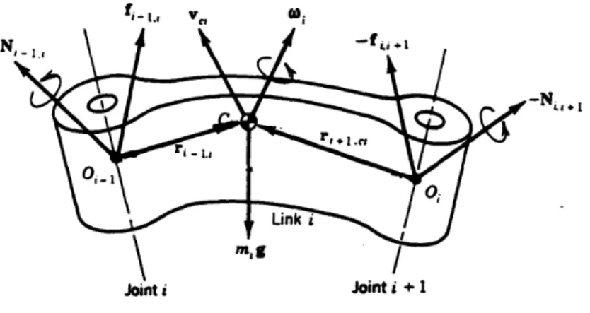
We begin by examining all of the forces and moments that act on each link of a robot with

(20)

on an arbitrary link (Asada and Slotine, 1986). The equations that govern the forces and moments acting on each link can be written.

N

Fig. 2.4: Forces and moments acting on link i

The balance of linear forces can be written

d(mvv) = f,.,_]- f,.,j+ +m,g, (2.1)

where mi is the mass of each link, v, is the velocity of the center of mass of each link,

fi~, is the force exerted by link i-i (the previous link), f, is the force exerted by link i+1 (the following link), g is the gravitational acceleration,

The balance of moments with respect to the centroid C, is given by

d(Ioj,) = Ni,,_ - N,,.,÷ + ri-_,j x f,_• - r,, x f. = ,..., (2.2)

where I is moment of inertial of each link, oi, is the angular velocity of the link, N,,-_ is the torque exerted by link i-1, Nij,, is the torque exerted by link i+1, r,_., is the position

vector of the center of mass from i-i joint, and r÷,,, is the position vector of the center of

mass from i+1 joint.

Consider the entire robot. We can write the position of the mass centroid as

R= M , (2.3)

(21)

where Mc = m and Mc is the total mass of the robot.

i=1

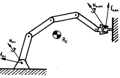
Figure 2.5 shows the forces and moments acting on the entire robot. The linear forces can be written as

dM

d (McRc) = fo., - fn,..n + Mcg, (2.4)

where f0., is the force exerted by the base on the robot and fn.. is the force exerted by the end-effector on the robot. The balance of moments of the entire robot can be written

d

-(L) = No.₁- N,,., + Ro._cx fo., - R.,,+c x f,,n+, - (Rc. xm,~,), (2.5)

dt _r=1

where L = Ico~ and No., is the torque exerted by the base on the robot, N..,, is the

i=l

torque exerted by the end effector on the robot, R.I,,c is the position vector of the mass

centroid with respect to the end-effector, and Rc,, is the position of the center of mass of each link with respect to the robot mass centroid. We observe from these equations that the linear forces at the base and end-effector are dependent upon the total momentum and not on the momentum of individual links.

Fig. 2.5: The forces and moments acting on a robot

(22)

The dynamic equations of motion of the entire robot can be expressed in terms of the actuator torques. Lagrange's Equations of motion of a n degree of freedom robot can be written

HO+h= h r, (2.6)

where coefficients H and h are functions of joint displacements 0 and joint velocities 6. For all dynamic task performed by our robot, the end-effector's location will be specified with m task coordinates:

rQ(t),...,rm(t). (2.7)

Once the end-effector's position is specified there exits (n-m) degrees of freedom which corresponds to the internal body motion shown in Figure 2.6. These remaining degrees of freedom can be represented by (n-m) independent generalized coordinates that satisfy the

Fig. 2.6: The internal movement of an n-m degree of freedoms

prescribed task coordinates. These generalized coordinate will be represented by

q = (ql,..., q,,_,,) . (2.8)

Associated with the generalized coordinates let us specify (n-m) generalized forces that act on the internal body mass (centroid) of the robot. These forces can be represented by

(23)

The dynamic equations of the internal body motion can be express as,

HR + hR = Q. (2.10)

By moving the internal body, generalized forces Q are created. These generalized forces

can be related to the robot's actuator torques with

Q=Dt, (2.11)

where D is a (n-m)x n matrix that distributes Q to z.

The forces and moments transmitted to the environment and the base are determined by the distribution of the actuator torques to produce the generalized forces Q. D will be

(n-m)xn dimensions which is rectangular and infers that the robot must be redundant.

2.4 The Redundancy Criterion

In order for a robot to create arbitrary dynamic forces at its end effector and base the robot must have the ability to move its end effector independently from the center of mass. This ability assumes that our robot will be defined as having the ability to move its end effector to arbitrary positions in its workspace independent of the dynamic forces created. This functionality can be achieved by designing the robot with a special form of redundancy. To be able to move the end effector separately from the center of mass, for each generalized task coordinate m there must be robot mass that can be controlled to move in the same direction or the opposite direction as the end effector. To achieve this criterion the robot should be designed such that for each generalized task coordinate nm of the end effector there exists at least two degrees of freedom n. This relationship can be

written:

n=2nm (2.12)

2.5 Computing Actuator Torques

For any dynamic task the force F, desired at the end-effector will be specified. The torque r, needed to bear the force F, borne by the structure can be computed from

(24)

r = JTFr,

(2.13)

where J is the Jacobian relationship of infinitesimal change in joint angle to endpoint displacement. We can express the total torque needed to bear the force and to account for the dynamic internal motion as

r= r, + zR,, (2.14)

where the internal body dynamics can be represented by Equation 2.10 and TR can be computed from

Q=DrR, (2.15)

To find an expression to relate these forces and torques. We examine the velocity relationship between the endpoint velocity and joint angles.

The end-effector velocity (m terms) can be represented in terms of the angular joint velocity of the robot using the Jacobian relationship of the robot as

i = J,O. _(2.16)

The velocity of the mass centroid of the robot (n-m terms) can also be represented in terms of the angular joint velocity of the robot using another Jacobian as

R = JRO. (2.17)

We can combine the two previous equations into one generalized expression.

[

I

=

J ,

(det J' 0)

(2.18)

**where J* = J. The angular joint velocities can be determined in terms of the velocity**

of the end-effector and velocity of the center of mass:

1

= J'

,,

JR

(2.19)

where ,r is the inverse Jacobian associated with the end-effector velocity and J,. is the

inverse Jacobian associated with the mass centroid velocity. Using the duality principle we can write the force that the end-effector applies and the generalized forces acting on the center of mass as

(25)

J .. (2.20)

If we examine the case of applying forces and assume that the end-effector is fixed ri = 0. Then the joint angular velocities of the robot can be computed by

e

= ,1R,

(2.21)

The torque needed by the actuators to apply a force at the end-effector and apply the generalized forces applied to the center of mass can be expressed with the following:

r= J F,+ JQ. (2.22)

Using Equations 2.10 and 2.22 the actuator torques needed to move the robot can be determined. The torques JrF, can be provided not only by the actuators but also by the internal body motion; JF, = r+ JrQ.

2.6 Centroid and End Effector Motion

In this section we will develop an analytical way of expressing the position of the end effector and centroid in terms of the joint displacements of our robot. An expression for the position of the end effector can be written as

r = Ikk, (2.23)

k=1

where !k is the pivot-to-pivot length vector of each link. The position of the end effector can be written in terms of its m components, as

r = [ryr.,...r, r . _1(2.24)

Each of the end effector coordinates can be written as

r, = fj(q,,q2,...,q,, j = 1,...m (2.25)

where r, represents the coordinates of the end effector and the q, are the joint displacements. The center of mass trajectory can be written (using Tepper and Lowen,

1972 notation) as

S(2

R = M myrsj, (2.26)

(26)

where M c is the total mass of the robot, mj is the mass of each link, rs, is the position

vector of each link.

The center of mass trajectory can be rewritten by expanding the position r•, of the center of mass of each link as

j-1

rS = r, + -1k (2.27)

k=1

and substituting this expression into equation (2.26) to give

R=

-

2M

m rj + k l. (2.28)

That is, for each link in a mechanism, a trajectory vector can be found that is represented

by the sum of the pivot-to-pivot length vectors (Ik) and the center of mass vectors (r,)

that define the distance from the end of a link to its center of mass. By multiplying each of these vectors by the mass of each link mi, summing them together, and then dividing by the total mass M _c, an expression for the center of mass R can be found.

The position of the center of mass can be written in terms of its m components as

R = ([4, PF,...PT]r. _(2.29)

These components are also a function of the n joint displacements

R, = gJ(q1,q2,...,q),

j

= 1,...,mn (2.30)

where the coordinates R, represent the center of mass position.

2.7 Inverse Kinematics

In this section we present a method for determining the joint displacements in terms of end effector and center of mass positions. In the previous section we found the end effector and centroid position in terms of the joint displacements. By meeting the redundancy criterion we have m coordinates for the end effector and n-mn coordinates for the centroid

and n joint generalized coordinates which would be equal to 2nm if the redundancy criterion was satisfied for a planar robot with two internal body degrees of freedom.

(27)

Therefore there are n equations and n unknowns. Let us represent the joint displacements

q71,...,q that satisfy both equations (2.25) and (2.30) as functions of ir and I•. Namely,

q, = h,(ri,...,rm, ,...,R,,), i = 1,...,n. (2.31)

If there exists a closed-form solution, this solution would give us absolute joint displacements for given positions of the end effector and center of mass.

Because of the form of Equations (2.25) and (2.30), it may not always be possible to find a closed form solution even though the system will always have n equations and n unknowns. For the cases in which a closed form solution for the joint displacements does not exist, numerical methods can be applied to calculate the joint positions.

Equation (2.30) gives the expression for the joint positions in terms of the centroid and end effector positions. To convert the time trajectory of the end-effector and centroid into joint position trajectories the end effector and centroid trajectories can be discretized into a number of positions and using Equation 2.31 a unique configuration of the robot could be computed for each of these positions.

In the following section we use the expression for the position of the end effector and centroid to find an ideal mass distribution for an exemplary robot. In this thesis we will examine the case of planar motion. To meet the redundancy criterion a four degree of freedom robot is needed. A serial chain of four links is selected for the design of our robot.

2.8 An Exemplary Robot Model

We would like to design our dynamic robot so that the center of mass is able to be controlled independently from the end effector. To begin with we examine a general mass distribution form of the serial four degree of freedom robot. For this robot shown in Figure 2.7, we can write the equations for the end effector using Equation (2.25):

4

x= l.cosi. _(2.32)

(28)

and

4

y= - .sin O, (2.33)

i=1

where x and y are the positions of the end effector, each 1, is the length of each link, and Oi are the joint displacements. We would also like to control the center of mass of our robot. Using Equation 2.30 we will define the positions of the center of mass:

4 X= Ai cos9i (2.34) i=1 and Y= Ai sin i, (2.35) i=

where X and Y are the positions of the center of mass and the A are constants that

(X.y)

Figure 2.7: General mass distribution form of 4 d.o.f. robot.

(29)

1 {

A

=

_{,I +}

_{M, + Im.}

_,

MT k=i

i= 1,...11

If we design our robot with most of the mass at M ₂then Al 11, / 2 /2, A3 0,

and A4 , 0 and our equation for the center of mass position reduces to:

and

(2.36)

X = ll cos0 1 + 12 cos0 2

Y = 11sin 01+ 12 sin 02. (2.37)

Now the center of mass equations have two unknowns and is directly solvable. By placing all or most of the mass in the M2 position the problem of controlling the robots center of

mass becomes a simple one.

For the rest of this thesis we will use this exemplary robot model. We will assume all of the links are mass-less. The links from the base to the mass M2 will be referred to as the

leg and links from M₂ to the end-effector will be referred to as the arm. Since most of the mass is located at M2 for this model this position will be referred to as the centroid of

the robot. Figure 2.8 show a diagram of the exemplary robot model considered in this thesis.

X(t)

(30)

The centroid coordinates X, Y can be used as independent generalized coordinates for distributing the internal body dynamics:

MIA + Mcg = Q, (2.38)

where Q are the generalized forces acting on the centroid which can be related to the actuator torques with the D matrix with Equation 2.15. The actuator torques for this example can be expressed as

r = (rl, ,r3, r4)T. (2.39)

The generalized forces acting on the centroid can be expressed in terms of its components:

Q = (F,,,, F)'. (2.40)

The velocity of the centroid can be written in terms of the joint velocities of the leg using the Jacobian relationship:

R =

Jo,,

where

0,

= _(01,0,)' . The velocity of the end effector can also be written

it = R + J,•,, where O, = (03, 0)' .

If we consider the task of applying forces, the end-effector velocity would be set

and the centroid velocity could be written in terms of the arm joint velocities: R = -J AI,.

Using the duality principle we can write the quasi-static forces borne by the robot i of the actuator torques. The forces produced on the centroid due to the leg torques can be expressed as

(2.41) (2.42) to zero (2.43) in terms actuator .J = JTFL, where r, = (r, r,)T. (2.44)

The forces produced on the centroid due to the arm can also be written

TA = -JAF, where -r =(rs,)T (2.45) The total generalized forces acting on the centroid are the sum of the forces produced by the arm and the leg which can be written

Q=FL+FA. (2.46)

(31)

For non-singular configurations the force produced on the centroid by the leg can be written in terms of the leg torques F, = JITr,. The forces produced by the arm on the

centroid can be written in terms of the arm torques FA = -JA T. The D matrix, which

relates the torques to the generalized forces (Q = Dr ) can be written

D

= [J~i,-J,']. (2.47)

For our example the D matrix has dimensions 2x4. It is possible for the leg or the arm to create the same force on the centroid. For each dynamic task the force created to the centroid needs to be distributed between the leg and the arm. To determine how these forces can be effectively distributed we examine the mechanical advantage.

Fig. 2.9 Forces acting on robot centroid

2.9 The Mechanical Advantage

We can represent the mechanical advantage by defining a transformer ratio that relates the input torque to the force borne by the robot (Asada and Cro-Granito, 1985). We can write this ratio as

A =

IL

(2.48)

(32)

where A is the mechanical advantage. To find our mechanical advantage in terms of the vector quantities we can compute the square of A. By substituting the torque/force relationship r = J'F into Equation 2.48, we can find the mechanical advantage in terms of

the force and the jacobian matrix:

FTF FTF

A" = = F (2.49)

zrr FrJJTF

The mechanical advantage varies depending on the direction of F. The maximum and minimum are provided by solving the eigenvalue problem.

JJTF =

AF,

(2.50)

where X is the eigenvalue of matrix JJT. Solving Equation 2.50 for X and plugging into Equation 2.49 our mechanical advantage will be

A=1, (2.51)

where the largest eigenvalue is the smallest mechanical advantage in the direction of the corresponding to the eigenvector and the smallest eigenvalue corresponding to the largest mechanical advantage:

1 1

1 A< 1•A _(2.52)

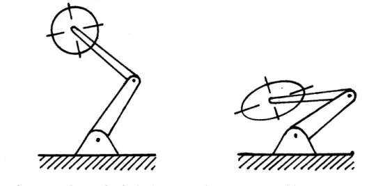
By assuming a constant power input this mechanical advantage can be represented by an ellipsoid. Where the largest eigenvalue corresponds to the minor axis and the smallest corresponds to the major axis. Figure 2.10 shows an example of a two dimensional robot in two configurations with an ellipsoid showing the direction of largest mechanical advantage.

(33)

The trajectory of the centroid and end effector can be derived using a combination of the previous sections. In Chapter 4 we compute an optimized trajectory using human motion as an initial estimate. Position trajectories can be computed by specifying the initial and

Fig. 2.10 The mechanical advantage of a two degree of freedom robot

final conditions on the motion of the centroid and end effector trajectories. Since there are an infinite number of initial and final conditions possible, human motion was studied in Chapter 3 to understand how humans take advantage of these conditions. Assuming that a trajectory can be computed for the motion of the centroid we will find expressions of how to relate this motion into joint displacements and finally, actuator torques.

2.10 The Human Form

The human body has many redundant degrees of freedom. This allows humans to be very flexible in accomplishing many tasks. Examining the horizontal plane of the human form, we find that the human motion in this plane can be modeled as a planar, four degrees of freedom series of links, with most of the body mass located between the arm and leg.

The robot we have designed can model the human form in the vertical plane observed from the side. By making this analogy it is possible to learn how to perform dynamic tasks by examining human motion.

(34)

In the following chapter human measurement is presented. Humans are measured performing two dynamic tasks, applying forces and dynamic lifting. By taking advantage of our model we: can simplify the measurement of this complex motion. We will limit our interest to only measuring the forces created at the base and end effector and the motion trajectories of the center of mass and end effector.

(35)

Chapter 3 Dynamic Force Generation

In this chapter human dynamic motion was studied to gain an understanding of how humans perform dynamic tasks. These measurements will be used to extract relevant schemes and to apply this knowledge to robotic motion. Humans were measured performing two exemplary dynamic tasks. We assumed a simple model of the human to explain forces production for these dynamic tasks. The human was modeled as a two dimensional string of n mass less links with the human's body mass located in the middle of the chain of links. Considering this model we were interested in measuring the position trajectories of only the humans center of mass and end effector. Also of interest was the forces produced through the end effector and the humans feet. These data of interest were measured for both tasks. This data measured will be analyzed and interpreted to understand the schemes used by humans to perform these dynamic tasks.

3.1 Human Production of Force

Human dynamic motion was studied in order to understand the physics of dynamic task performance, in this section an exemplary task of applying forces is considered, and critical features of human task strategies will be obtained from this example. Figure 3.1 shows the simple task of opening a heavy door. As we experienced, we utilize the counteraction of the body motion to generate a large force. Namely, first we push the body away from the door, and keep increasing the momentum in that direction (Fig. 3.1-a). This continues until the arm is nearly extended (Fig. 3.1-b). At the time of full arm extension, which is a singular configuration of the arm, the body momentum is decreased abruptly, creating an enormous pulling force at the door knob. The forces generated

(36)

dynamically as in this exemplary task are significantly larger than the ones generated statically, that is, the force created without large momentum changes.

It is highly desirable to understand how a human is capable of producing dynamic forces and to study human dynamic motion so we can apply this knowledge to determining trajectories for a robot that is capable of a similar dynamic motion.

a)

b)

Figure 3.1: Human door opening task

3.2 Measurement of Human Dynamic Force

3.2.1 Experimental Setup

To measure dynamic forces produced by humans an experiment of opening a stuck door was chosen. The experiment was performed using a door that was instrumented with a force sensing handle. This door was secured shut during the experiment. Horizontal forces on the floor were measured using a force sensing floor tile. Nine subjects participated in the experiment. Each subject was asked to stand on the force tile, to hold on to the door handle, and on cue (when sampling was initiated ) to pull as hard as

(37)

possible with a constant force for three seconds, then to pause, and then to apply as high a force as possible using any means. Data were collected for 10 seconds for each subject.

A 20 Hz sampling rate was used to collect the forces measured. To measure the motion of the subjects approximate center of mass, each subject was recorded from the side with a video camera.

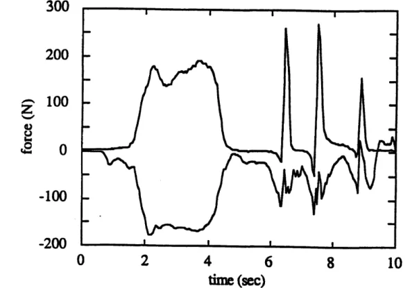
3.2.2 Results

Figure 3.2 and 3.3 show typical results of the force measurements collected. The upper line is the measured force applied to the door handle. The lower line shows the force measured from the floor tile sensor. Positive force indicate a force in a direction away from the door ( parallel to the floor ). The initial (3 second) quasi-static part of the force data can be seen as the mirror image forces shown in figure 3.2 the

U #0

300

200

100

0 -100

-200

2

4

6

8 time (sec)

10

Figure 3.2: Force measured for subject I

second part of the force measurements can be seen as a repeating pattern of peak forces. Each pattern begins with a small force which can be seen in Figure 3.2 labeled fl and then

(38)

a large force created to the door handle labeled h l followed by another small force labeled f2. Figure 3.3 also exhibits similar patterns.

2

4

6

8 time (s)

Figure 3.3: Force measured for subject 2

2

4

6

8 time (sec)

Figure 3.4: Position measured for subject 2

10

400

300

200

100

0 -100

-200

-300

0.1

0 -0.1

-0.2

-0.3

-0.4

-0.5

(39)

The video tape of the subject motion was digitized using a software package called Image. The results of this digitization are shown in Figure 3.4. The graph shows the horizontal displacement of the subject's approximate center of mass. Zero is defined by the initial starting position of the subject's motion.

3.2.3 Discussion

During the initial quasi-static phase of the measurements an expected mirror image force on the floor and door in both Figures 3.2 and 3.3 can be seen. After the short pause the second phase of the force production can be seen. In each case the subject always resorted to a dynamic method for the second phase of the sampling period. Several dynamic force attempts can be seen applied to the door. For each of these dynamic forces

a pattern of forces on the door and on the floor can be seen. The beginning of each

dynamic force begins with a force pushing on the floor tile toward the door. This force can be seen in Fig. 3.2 ( labeled fl). The push on the tile is created by the subjects legs pushing their body away from the door, accelerating their body mass. As the subjects arm approaches a completely extended configuration ( a singular configuration ), the subjects body is decelerated rapidly with only a relatively small torque required by the subject's arm muscles. This deceleration results in a large force borne through the subjects arm to the door handle. This force can be seen as hi in Figure 3.2. This large force is exerted for the time of the subjects body being decelerated, while the arm is near its extended singularity. After this force has been created a recovery force labeled f2 exerted by the legs of the subject decelerates the subjects body back to rest at the starting position. The body is now in a configuration to repeat the task.

The peak force produced to the door during the dynamic phase is 50% greater than the peak force produced during the quasi-static phase. In addition, the initial pushing forces and recovery forces produced to the floor are 45% less than the forces on the floor created during the quasi-static phase. This demonstrates the ability for a human to direct forces. Directing forces could be an important tool in the field of robotics and shows the need to understand this dynamic method.

(40)

Figure 3.4 shows the motion of subject 2's body This motion shows the acceleration and deceleration of the subject approximate centroid. This motion can be seen to be held constant for the quasi static phase and shown to oscillate for the dynamic phase. It is this oscillating motion that permits the dynamic case to produce large forces.

The door opening task is a simple example since the end-effector is fixed in space. Humans can perform much more complex tasks by utilizing the whole body dynamically and effectively. In the following sections we will focus on weight lifting as an exemplary task.

3.3 Analysis of Weight Lifting Athletes Using Dynamic Lift

Trained athletes are capable of lifting as much as three and a half times their weight to a position over their head very quickly. This is possible by using the so-called "dynamic lifting technique" in which the whole body motion is precisely coordinated with the barbell motion.

Figure 3.5 shows the basic form of the 'power clean' lift. The human subject begins with his knees bent in. a crouched position shown by configuration c 1l. The mass is lifted with a moderate force until the

()

P

c2 c3 c4

Figure 3.5: The 'power clean' dynamic lift

mass reaches the knees (c2). After this point, the greatest force is applied to the mass. This pull is accomplished by the subject's back thrusting backward and legs thrusting the

(41)

body upward. The mass is pulled up by the arms, which at this time are fully extended (acting as ropes connected to the shoulders). This thrust can be large enough for the subject and the mass to become airborne. The subject, while airborne, continues to pull on ithe mass (c3). This pulling causes the mass to continue moving upward and brings the lifter back in contact with the ground. After reaching this point, the lifter is no longer able to apply a substantial force to the bar because of the configuration of his arms. Although no large force is applied, the bar continues moving upward as a projectile and approaches the top of its trajectory. During this time the subject bends his knees, dipping to a semi-squat, and positions himself under the mass (c4). The mass then comes-to rest on the subject's chest, with his arms in a completely bent configuration. The subject then pushes hiimself and the mass upward with his legs until the subject is standing with the mass at his chest (c5). In weight lifting competition the lifter would then produce the 'jerk' part of the lift which is the push of the weight above the lifters head. For our experiment only the 'power clean' part of the lift will be measured and analyzed.

3.4 Measurement of Athletes' Lifting Motion

3.4.1 Experimental Setup

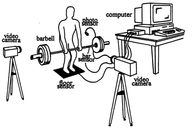
As shown in Figure 3.6, the subjects stood on a force plate to measure the forces between the subjects body and the floor, and the bar was instrumented with a force sensor to measure the forces between the subject's body and the lifted mass. Two video cameras were used to record the motion of the subject. One was placed directly in front of the lifter and the other was placed on the side of the lifter. The subject's motion was recorded from the front with a high speed (200 frames/sec) video camera placed 23 feet from the subject. The side motion was recorded using a normal speed (30 frames/sec) video camera placed :20 feet from the subjects. Markers were placed on the joints and approximate centroid of the subject's body as well as on the lifted mass. Sampling of force information was done using data acquisition software, Lab View, on a Macintosh IIci with a sampling rate of 200 Hz. The subject informed us when he was ready and then the motion was recorded for five seconds. At the beginning of the sampling period a photo

(42)

sensor was tripped in the view of both video cameras and the signal was recorded by the computer. This action was done so that the video and force data could be synchronized during analysis.

video

camera

Figure 3.6: Experimental setup

3.4.2 Results

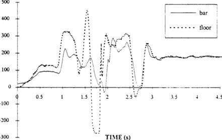
Figure 3.7 shows the time profile of the force measurements taken during a 205 lbs 'power clean'. For comparison purposes the forces on the floor has been inverted and subject A's weight has been subtracted. Notice the two first peaks marked pl and p2 respectively and the dip between these peaks marked dl. Following dl there is a small dip d2 that occurs on the bar at the same time as p2. After this small dip there is a small peak force p3 produce on the bar. This detail is followed by a large drop in force on the floor marked d3, followed by the drop of force on the bar marked d4. After these drops there is a large sharp force on the floor labeled p4 followed by another peak force on the bar labeled p5. These peaks are followed by oscillations and another drop in forces at d5

(43)

followed by a peak force p6, although in this case the force on the floor and the force on the bar are occurring approximately in phase.

-1 p4 p5 bar . --- floor AC d3 TIME (s)

Figure 3.7: Forces measured during subject A's lift

Figure 3.8 shows the force profile during a 225 lbs 'power clean' by subject B. Again for comparison purposes the force on the floor has been inverted and subject B's weight has been subtracted. It is apparent that both of these subjects have relatively the same signature force curves for this lift with deviations in the magnitude of the peaks.

b- bar S-... tloor -100 -200 -300 _{TIME (s)}

Figure 3.8: Forces measured during subject B's lift

300 100 0 t600 T 500 t 400 4 :300 200 100 0 -100 -200_-200 5 300 --- --i

(44)

Figure 3.8 shows the force profile during a 225 lbs 'power clean' by subject B. Again for comparison purposes the force on the floor has been inverted and subject B's weight has been subtracted. It is apparent that both of these subjects have relatively the same signature force curves for this lift with deviations in the magnitude of the peaks.

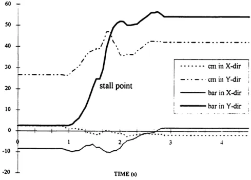
The side view of subject A's lift was digitized using a software package called Image. The results of this digitization are shown in Figure 3.9. The graph shows the vertical displacement of the bar and subject A's approximate center of mass. There is a small flat spot in the trajectory of the bar labeled stall point.

Another feature to notice is the peak of the subjects centroid as the bar continues to move upward. After this peak the trajectory of the centroid and the bar move almost in unison.

3.4.3 Discussion

The patterns in the graph of measured forces provide useful information as to how a person lifts dynamically. If we examine Subject A's lift in Figure 3.7 we find a distinct pattern that Subject A repeated every time he lifted during the experiment.

60 -50 40 30 20 10 0 -10 2- 0 ₁ lAVr. ~s)

Figure 3.9: The vertical motion of the subject A's center of mass and bar

(45)

-20--·-At the beginning of the lift, the force on the floor can be seen to start slightly before the force on the bar. The force on the floor then continues to increase and smoothly levels off, and the force on the bar abruptly peaks and then levels off (pl in Figure 3.7). This detail shows the transfer of force to the mass through the subject's arms. The subject is able to transfer the large force produced by his legs through his arms since the subject's arms are in a singular configuration (see c2 in Figure 3.5). This configuration allows the structure of the subject's arms to bear the force. Once the mass is accelerated the force in the bar goes down compared to the force on the floor. The first dip dl will be referred to as the stall point. This point is the instant when the weight reaches knee height, just before the large pull occurs. The stall point can also be seen in the trajectory of the bar in Figure 3.9. The body of the subject is now approaching a singular configuration and is capable of applying a very large thrust upwards. This thrust is clearly seen by the force produced on the floor by peak p2 shown in figure 3.7. During this peak (p2) the force on the bar increases slightly after the stall point (dl). Then there is a small dip (d2) which shows the transfer of force from the arms acting like ropes to the force (p3) created by the arms starting to pull on the mass as the body of the subject begins to leave the ground (shown in Figure 3.5 by configuration c3). During this part of the lift the body of the subject is now decelerating upward and begins to accelerate downward. The force on the floor (shown in Figure 3.7 by dip d4) becomes negative since we have subtracted the lifters weight. It is during this part of the lift that the subject is removing the energy stored in the mass of his body and transferring it through his arms to lift the mass. This can be seen in the trajectory graph (Figure 3.9) of the subject's body moving up and then down while the trajectory of the mass continues to move upward. This is similar to the door opening task strategy in which the body is first accelerated and then decelerated so that the bodies kinetic energy is transferred through the arm. After this motion in the lift, the subject is not capable of giving the mass any additional force since his arms are no longer near a singular configuration shown by configuration c4 in Figure 3.5. In this configuration during a quasi-static lift it would be necessary for the subject's arm muscles to bear the entire weight . At this time the subject comes abruptly back in contact with the ground.

(46)

This can be seen in the third very sharp peak force (p4) that occurs on the floor in figure 3.7. Since the mass is hanging instantaneously the subject positions himself at this time to accept the weight at his chest. The force peak on the bar that follows (p5) is the weight coming down on to the subject's chest and the oscillations that follow are caused by the vibration of the mass and the bar's compliance. The subject's arms are now able to bear the load since they are in another singular configuration. Once these oscillations stop the lifter can push upward using his legs. The lifter lifts, with the weight at his chest, from the crouched position to standing straight shown by position c5 in Figure 3.5. This simultaneous motion can be seen in the trajectory graph (Figure 9) between 2.25 sec and 3.0 sec. In Figure 3.7 there is a large dip (d5) that occurs simultaneously for both the force on the floor and the force on the bar. This dip is caused from the upward 'jump' after the push from the crouched position. The landing from this 'jump' can be seen as the next large peak (p6) followed by the oscillation of the subject and mass coming to rest.

Design and analysis of robots that perform dynamic tasks using internal body motion