Shape, size, pressure and matrix effects on 2D spin crossover nanomaterials studied using density of states obtained by dynamic programming

HAL Id: insu-02953987

https://hal-insu.archives-ouvertes.fr/insu-02953987

Submitted on 18 Nov 2020

HAL is a multi-disciplinary open access archive for the deposit and dissemination of sci-entific research documents, whether they are pub-lished or not. The documents may come from teaching and research institutions in France or abroad, or from public or private research centers.

L’archive ouverte pluridisciplinaire HAL, est destinée au dépôt et à la diffusion de documents scientifiques de niveau recherche, publiés ou non, émanant des établissements d’enseignement et de recherche français ou étrangers, des laboratoires publics ou privés.

Shape, size, pressure and matrix effects on 2D spin

crossover nanomaterials studied using density of states

obtained by dynamic programming

Jorge Linares, Catherine Cazelles, Pierre-Richard Dahoo, Devan Sohier,

Thomas Dufaud, Kamel Boukheddaden

To cite this version:

Jorge Linares, Catherine Cazelles, Pierre-Richard Dahoo, Devan Sohier, Thomas Dufaud, et al.. Shape, size, pressure and matrix effects on 2D spin crossover nanomaterials studied using density of states obtained by dynamic programming. Computational Materials Science, Elsevier, 2021, 187, pp.110061. �10.1016/j.commatsci.2020.110061�. �insu-02953987�

Shape, size, pressure and matrix effects on 2D Spin

Crossover nanomaterials studied using density of states

obtained by dynamic programming

Jorge Linares[1*,2] , Catherine Cazelles[3], Pierre-Richard Dahoo,[4,5] , Devan Sohier,[6] Thomas Dufaud,[6,7]] Kamel Boukheddaden[1]

1

Université Paris-Saclay, UVSQ, CNRS, GEMaC, 78000, Versailles, France

2

Departamento de Ciencias, Sección Física, , Pontificia Universidad Católica del Perú, Apartado 1761 - Lima, Peru

3

Université Paris-Saclay, UVSQ, IUT de en-Yvelines, 78200 Mantes-la-Jolie

4

Université Paris-Saclay, UVSQ, CNRS, LATMOS, 78280, Guyancourt, France

5

Université Sorbonne, UVSQ, CNRS, LATMOS, 78280, Guyancourt, France

6

Université Paris-Saclay, UVSQ, Laboratoire d’informatique Parallélisme Réseaux Algorithmes Distribués, 78035, Versailles, France.

7

Université Paris-Saclay, UVSQ, CNRS, CEA, Maison de la Simulation, 91191, Gif-sur-Yvette, France

*

Corresponding author.

jorge.linares@uvsq.fr

E-mail address :

Abstract: In the present work, numerical simulations based on a new

algorithm specific for 2D configurational topology of spin crossover nanoparticles embedded in a matrix are presented and discussed in the framework of the Ising-like model taking into account for short- (J) and long-range (G) interactions as for surface effects (L). The new algorithm is applied to calculate the density of states for each macro-state, which is then used to calculate exactly the thermal behavior of spin-crossover nanoparticles under an applied pressure. We find that the pressure plays the role of a conjugate parameter of the temperature. Thus, increasing pressure is somehow equivalent to reducing the temperature

1. Introduction

Spin-crossover (SCO) compounds which belong to the field of molecular magnetism are typical examples of a first-order phase transition with thermal hysteresis[1-9]. Fe(II) based SCO complexes are among the most studied switchable molecular materials in which the spin transition takes place between two spin states, namely the high spin (HS) state, stable at high temperature, and the low-spin (LS) state, which is stable at lower temperature. It is quite well known that in Fe(II) d6 spin-crossover complexes, the electronic structure of the HS state is

with a spin S=2, whereas that of the LS state is with a spin S=0. Because of the

antibonding character of the orbitals, the strength of the bond between the Fe(II) and the ligand is weaker (resp. stronger) in the HS (resp. LS) state with two (resp. zero) electrons in the orbital. Consequently, the bond length between the ligand and the Fe(II) metal centre is longer in the HS than that in the HS by about

[2].From the elastic rigidity point of view, the SCO materials are then soft and distortable in the HS state and rigid in the LS state, which has a higher bulk modulus than the HS state. It is important to mention for the non-specialist reader that the SCO solids are paramagnetic in the HS and do not show magnetic ordering, while they are diamagnetic in the LS state. The reason of the absence of the magnetic ordering can be attributed to their molecular structures, which leads to large distances (

nm) between the iron sites.

The competition between the spin states and the elastic interactions between the molecular units is therefore responsible for the resulting “bi-stable” character of the spin-crossover solids. Indeed, due to the local volume change accompanying each spin transition of the molecules, long- and short-range range elastic interactions[10-13] take place between the SCO units causing their cooperative hysteretic first-order thermal transitions, driven by the large entropy (originating from spin and vibrations) of the HS state compared to that of the LS. In this respect, experimental and theoretical studies of solid state cooperative effects have become a very popular topic and as a result the investigation on the potential industrial applications offered by SCO compounds is worldwide.

One of the quest in many research groups concerns new materials for information storage and these compounds as bistable materials are the focus of research work. Indeed, spin transition materials have been studied for a long time for their thermally[2,3], pressure[14-17], electric[5], magnetic-field[18] , and light[19] induced bistabilities. They have potential applications as sensors of pressure and temperature[7] but also as displays and actuators[8] and recently they have shown abilities as materials for molecular spintronics[1] due to the interplay between the conducting properties and their spin states. Since ten years now, nanoparticles of spin-crossover materials (SCO) have been synthesized and studied with the aim to understand how the reduction of the size influences their switching properties. In addition to the study of the size dependence of ensemble of free nanoparticles, other investigations related to nanoparticles embedded into polymeric matrices have also been developed in order to clarify the role of the environment or surface nanoparticles on their thermal behaviors[20-22]. Several experimental results demonstrated that the physical properties of the nanoparticles crucially depend on their size, shape and environment and a large number of models have been proposed to mimic the experimental facts.

In this work, we will focus solely on the modeling of thermal and pressure effects in 2D SCO lattices. From the theoretical side, the modelling of SCO phenomena helps to get new insights

on the physical properties of SCO nanoparticles, particularly those displaying phase transitions, whose behavior as a function of their size and their interaction parameters play an important role in the control of the switching features of these complex materials, with the ultimate goal to help to design novel and specific systems with tailored properties.

From the general point of view, the modeling of phase transition allows a better understanding of the microscopic physical processes from which originates the cooperativity of the materials, as well as the nature of the interaction’s mechanisms (magnetic, elastic, electrostatic, electronic …) involved during their transformation. In spin-crossover materials, the elastic interactions have been identified as playing a key role in their macroscopic thermo-, photo- and piezo-transformations between LS and the HS states. These elastic interactions are mainly due to the molecular volume change accompanying the spin transition at the microscopic scale, which deploys in the long-range way over the lattice through acoustic phonons. The long-range elastic interactions which stabilize homogeneous phases in most of the cases, compete with the ligand field which has a local and electronic nature, following which the thermal-dependence of the HS fraction curve may exhibit several shapes, among which, one can quote: (i) first order phase transitions with thermal hysteresis, (ii) incomplete spin transitions characterized by the presence of residual HS fractions at low-temperature, (iii) gradual and stepwise one with two or three steps, as well as re-entrant transitions. In the special case of SCO nanoparticles, these behaviors can be obtained by changing the size of the nanoparticles, which influences the balance of interactions between the bulk and surface contributions as well as other effects related to external stimuli (light, pressure etc.)

The manuscript is organized as follows: in Sec. 2 the model and the principles of calculations are explained. Sec. 3 summarizes the numerical simulations’ results on 2D lattices and a detailed discussion of the behavior of the high-spin fraction under various stimuli. Finally, in Sec. 4 we conclude and draw some possible extensions of this work.

2. Model and principle of calculation

Various physical techniques and methods, such as magnetic, optical spectroscopy, X-ray and neutron diffraction and heat capacity measurements are used to study the switching properties of SCO materials. The switching process from LS to HS triggered by an external stimuli, have been simulated using different types of models such as, the Ising-like model

[23-26]

, the atom-phonon coupling[27], mechano-elastic[13,28], electro-elastic [29,30], vibronic [31,32], elastic [33].

Below, we first present the Ising-like model, with includes short- (J) and long- (G) range interactions together with the interaction (L) between surface molecules with the surrounding matrix. The density of states, needed to perform our numerical simulation is obtained with a new algorithm that will introduced and described in details.

2.1 Extended Ising Model with short- and long-range interactions

Forty years ago, Wajnflasz and Pick[23] proposed the use of the Ising model to describe the spin transition behavior in which only “short-range interaction” between the spin-crossover sites were considered. Later, Bousseksou et al.[24] who made a thorough analysis of this model in the mean field approximation, reproduced, by introducing ferro-magnetic like and short-range "antiferromagnetic-like” interaction, the double-step character of some experimentally observed spin transition solids. Furthermore, Linares et al.[25] , by the

introduction of a long range interaction in the Hamiltonian besides the short range interaction, were able to reproduce hysteresis in 1D compounds, as well.

With these contributions, the Hamiltonian now includes the short- and long-range interactions to which we added an energetic contribution “L”[11-34-35] , «to the ligand-field of edge molecules of a SCO nanoparticle ». This term allows us to explicitly take into account for the interactions between molecules on the edge and the environment in close contact, which weaken the molecular field.

In addition to these energetic terms, the present study considers also the contribution of an external isotropic pressure, P, whose effect is to renormalize the gap energy Δ (energy difference between HS and LS states), the effective expression of which is given by 𝛥 + 𝑃 × 𝛥𝑉 , where 𝑃 is the applied external pressure and 𝛥𝑉 = 𝑉_𝐻𝑆− 𝑉_𝐿𝑆 is the volume change of the material between the HS and the LS states.

The behaviour of SCO nanoparticles under the external constraints of pressure or surface effects as experimentally studied by one of the authors[15-16] is simulated using an Hamiltonian operator based on an extended Ising model. Simulation is performed by applying the algorithm described in section 2.2 to the Hamiltonian of the extended model described in a previous work by some of the present authors [11,36] and which is given in equation 1 for self-consistency and clarity.

𝐻 =∆ + 𝑃 × ∆𝑉 − 𝑘𝐵𝑇 𝑙𝑛 𝑔 𝜎_𝑖 𝑁 𝑖=1 − 𝐺 𝜎𝑖 𝑁 𝑖=1 < 𝜎 > −𝐽 𝜎𝑖 <𝑖,𝑗> 𝜎𝑗− 𝐿 𝜎𝑘 𝑀 𝑘=1 ( )

In (1), 𝜎 is a fictitious operator, which has two eigenvalues +1 and -1, respectively associated with the HS and LS states. 𝑇 is the temperature,

𝑔

is the degeneracy ratio between the HS and LS states and 𝑘_𝐵 is the Boltzmann constant, 𝜎_𝑘 represents the fictitious spin state of the molecules on the edge.

The way Hamiltonian (1) is expressed allows separation of the coupling terms pertaining to the interactions of the environmental matrix at the core and the edge as illustrated in figure 1, in terms of black dots and red dots respectively. It is then straight forward to discriminate the effects of these terms on the simulated behavior of the material.

● ● ● ● ● ● ● ● ● ● ● ● ● ● ● ● ● ● ● ● ● ● ● ● ● ● ● ● ● ● ● ● ● ● ● ● ● ● ● ● ● ● ● ● ● ● ● ● ● ● ● ● ● ● ● ● ● ● ● ● ● ● ● ●

Figure 1: Schematic view of the SCO nanoparticle. Black dots are bulk sites, while red dots

are surface atoms that have specific interaction with their immediate environment.

The first right hand side term in (1), containing the effective ligand field renormalized by the pressure effects, is a one site contribution which concerns all (bulk and surface) lattice atoms. There, 𝑔 =𝑔𝐻𝑆

𝑔𝐿𝑆 represents the ratio of the degeneracies between the HS and LS states. The

volume change accompanying the spin transitions of the molecules is accounted for by the second term of equation (1) which models the long range elastic interactions, which spreads throughout the lattice. This effect is taken into account here through the uniform and infinite long-range interactions, written as a mean-field term, in which

< 𝜎 >

is the average magnetization per site. The third contribution expresses short-range interactions between the SCO species, while the last term pertains to the coupling of surface molecules with their specific environment. Finally, parameters N and M describe the total number of molecules in the lattice and at the surface or edge respectively.

For self-consistency we recall the definition of the macroscopic parameters[36] m (“total magnetization”), s (pairwise lattice correlations) and c (“surface magnetization”), used to describe thermodynamic properties and which are implemented as such in the algorithm of section 2.2.

𝑚 = 𝑁_𝑖=1𝜎_𝑖 = 𝑁 < 𝜎 > 𝑠 = _<𝑖,𝑗>𝜎_𝑖𝜎_𝑗 𝑐 = 𝑀_𝑘=1𝜎′_𝑘 (2)

Equation 1 can then be expressed in terms of m, s and c as in equation 3:

𝐻 = .∆+∆𝑉.𝑃−𝑘𝐵𝑇 𝑙𝑛 𝑔

2 − 𝐺 < 𝜎 >/ 𝑚 − 𝐽𝑠 − 𝐿𝑐 (3)

The number of configurations corresponding to the same m, s and c values leads to the calculation of the density of macrostates, 𝑑(𝑚, 𝑠, 𝑐) from which the thermodynamic properties of the system of nanoparticles can be determined. If the density of macrostates is denoted by 𝑑(𝑚_𝑖𝑠_𝑖𝑐_𝑖), then

< 𝜎 >

the average value of the operator 𝜎 can be calculated from equation 4[31]. < 𝜎 >= 𝑚𝑖 𝑁 𝑁𝐿 𝑖=1 𝑑(𝑚𝑖𝑠𝑖𝑐𝑖)𝑒𝑥𝑝 −𝛽(−ℎ𝑚𝑖−𝐽𝑠𝑖−𝐿𝑐𝑖) 𝑑(𝑚𝑖𝑠𝑖𝑐𝑖)𝑒𝑥𝑝 −𝛽(−ℎ𝑚𝑖−𝐽𝑠𝑖−𝐿𝑐𝑖) 𝑁𝐿 𝑖=1 (4) Where, 𝛽 = 1

𝑘𝐵𝑇 and NL is the number of possible *𝑚, 𝑠, 𝑐+ configurations. The field-like term, h, appearing in Eq. (4) is expressed as

ℎ = − .∆+∆𝑉.𝑃−𝑘𝐵𝑇 𝑙𝑛 𝑔

The HS fraction, 𝑁_𝐻𝑆, that is the probability to occupy the HS state is given by the equation,

𝑁_𝐻𝑆= +<𝜎> (6)

𝑁

_𝐻𝑆is determined from equation 4 using values calculated for 𝑑(𝑚, 𝑠, 𝑐), and the different corresponding *𝑚, 𝑠, 𝑐+configurations both by Monte Carlo Entropic Sampling[26] and by the algorithm described in section 2.2

Under the assumption that the transition temperature of the system is the result of a null total effective ligand-field, the transition temperature, 𝑇_𝑒𝑞 of a square lattice can be calculated from:

∆+∆𝑉.𝑃−𝑘𝐵𝑇𝑒𝑞𝑙𝑛 𝑔

2 × (𝑁𝑥− )

2₊∆+∆𝑉.𝑃−2𝐿−𝑘𝐵𝑇𝑒𝑞𝑙𝑛 𝑔

2 × (𝑁𝑥− ) = (7)

Where the number of core and edge sites are given by (𝑁_𝑥− ) and (𝑁_𝑥− ) respectively when the length of one side of the square is given by 𝑁𝑥.

As shown by Muraoka et al.[9], the transition temperature 𝑇_𝑒𝑞 can be expressed in terms of 𝑇𝑒𝑞𝑠𝑢𝑟𝑓

and 𝑇𝑒𝑞𝑏𝑢𝑙𝑘 , the surface and bulk transition temperatures respectively as :

𝑇_𝑒𝑞=𝑁𝑐 𝑁 𝑇𝑒𝑞 𝑏𝑢𝑙𝑘₊𝑁𝑠 𝑁𝑇𝑒𝑞 𝑠𝑢𝑟𝑓 (8) where 𝑇𝑒𝑞𝑏𝑢𝑙𝑘=∆+∆𝑉.𝑃_𝑘 𝐵𝑙𝑛 𝑔 𝑎𝑛𝑑𝑇𝑒𝑞 𝑠𝑢𝑟𝑓₌∆+∆𝑉.𝑃− 𝐿 𝑘𝐵𝑙𝑛 𝑔 (9)

To study the effect of the interaction between the nanoparticles at the surface and the matrix environment through the coupling term L, different cases have been considered. Keeping the temperature at a fixed value and varying the pressure (isothermal conditions) and keeping the pressure at a fixed value and varying the temperature (isobaric conditions) for L=0 (absence of surface effects) and 𝐿 ≠ (including surface effects).

2.2 Derivation of the density of states d[m,s,c] from dynamic programming algorithm

For a number of atoms

𝑛

, the computation of 𝑑(𝑚, 𝑠, 𝑐) by the naive enumeration algorithm is of complexity 𝑂( 𝑛), which is considered intractable even at nanoscale. Stochastic approach with Monte Carlo Metropolis method or Monte Carlo Entropic sampling is normally used[26].

Nevertheless, considering only

𝑛

, it is possible to reduce the complexity and perform exact computation based on the Transfer Matrix method as it has been proposed to compute 𝑑(𝑠) in the ferro-magnetic field[37].

We propose here a general technique based on a dynamic programming approach[38] that, in a sense, extends the Transfer Matrix method[39] and enables to compute 𝑑(𝑚, 𝑠, 𝑐) for any

geometry. It leads to a parallel algorithm with complexity 𝑂 .𝑛52 𝑛/ in time and space. This exact density of states has been used for the study of SCO compounds firmly expected for the design of a three-state electronic storage system[40].

In this section, we propose a general algorithm for the exact computation of the density of states 𝑑(𝑚, 𝑠, 𝑐) which is denoted by 𝑧(𝑚, 𝑠, 𝑐) in the following and then explain the particular case of the 2D grid.

Problem statement

We consider a set 𝐴 of atoms, each of spin

±

. Note 𝜎_𝑎 the spin of atom 𝑎 ∈ 𝐴. Pairs of atoms may be linked, note 𝐿 ⊂ 𝐴 × 𝐴 the set of pairs of adjacent atoms. The considered set of atoms has a border 𝐵 through which it interacts with the outer world.

To compute the Hamiltonian associated to this situation, one needs to compute the number 𝑧(𝑚, 𝑠, 𝑐) of configurations characterized by the three already defined quantities, which are recalled in the following :

-

𝑚 = _𝑎∈𝐴𝜎_𝑎, is the sum of all spins;

-

𝑐 = _𝑎∈𝐵𝜎_𝑎, is the sum of the spins at the edge of the grid;

-

𝑠 = (𝑎,𝑏)∈𝐿𝜎𝑎𝜎𝑏, is the sum of the product of spins of adjacent atoms.

Let 𝜎_𝑎′ ₌ +𝜎𝑎_{, which is 1 if 𝜎}

𝑎= , and 0 else. Then, let

-

𝑚′ ₌

𝑎∈𝐴𝜎𝑎′ = |𝐴|+𝑚

, the number of atoms with spin 1;

-

𝑐′₌

𝑎∈𝐵𝜎𝑎′ = |𝐵|+𝑐

, the number of edge atoms with spin 1;

-

𝑠′₌

(𝑎,𝑏)∈𝐿(𝜎𝑎′ − 𝜎𝑏′) =|𝐿|+𝑠 (because 𝜎𝑎𝜎𝑏 = − (𝜎𝑎− 𝜎𝑏) = − (𝜎𝑎′ −

𝜎_𝑏′) ), the number of « unbalanced » edges, the extremities of which have different spins;

-

𝑧′_(𝑚′_{, 𝑠}′_{, 𝑐}′_{) the number of configurations with given 𝑚}′_{, 𝑠}′ _{and 𝑐}′_.

From these definitions, we have the following relations: 𝑚 = 𝑚′− |𝐴|, 𝑐 = 𝑐′− |𝐵| and 𝑠 = 𝑠′− |𝐿|, and 𝑧(𝑚, 𝑠, 𝑐) = 𝑧′.|𝐴|+𝑚 2 , |𝐵|+𝑐 2 , |𝐿|+𝑠 2 /.

Thus, the knowledge of 𝑧′ _{is sufficient to compute 𝑧. From the equalities above, one sees}

that the parity of 𝑚,

𝑠

and

𝑐

only depends on that of

|𝐴|

,

|𝐿|

and

|𝐵|

. In other words, for a given particle topology, indexing the 𝑧 array with 𝑚,

𝑠

and

𝑐

imposes that seven elements in eight are zero; the 𝑧′ _{array is much denser and thus allows a better exploitation of the memory}

available. In the following of this section, we compute 𝑧′ _{and, for the sake of simplicity, drop}

the primes.

Dynamic programming algorithm

When attaching a new atom

𝑎

to the set 𝐴, 𝑚 is incremented if the new atom has spin 1,

𝑐

is incremented if the new atom is an edge atom and has spin 1, and

𝑠

increases by the number of atoms with a different spin to which the new atom is attached. Thus, computing the new (𝑚, 𝑠, 𝑐) requires to know its former value but also, in order to compute

𝑠

, the spins of the atoms to which

𝑎

is attached.

Generalizing this observation, we can compute the array 𝑧𝐴(𝑚, 𝑠, 𝑐) for a set of atoms 𝐴 by

adding the atoms in 𝐴 one after the other, and remembering the number of configurations with a particular value of (𝑚, 𝑠, 𝑐) and of each atom not all of the neighbours of which have yet been attached. Thus, note 𝑧

𝐴′(𝑚, 𝑠, 𝑐, 𝜎) the number of configurations with given 𝑚,

𝑠

,

𝑐

for

a given set of atoms 𝐴′, and ∀𝑎 ∈ 𝐴′′, 𝜎(𝑎), 𝐹 being the set of nodes in 𝐴′ that have neighbours in 𝐴 ∖ 𝐴′.

Thus, with 𝐹 the set atoms to which

𝑎

is attached, and to which no other nodes will be attached, if further atoms will be attached to

𝑎

:

𝑧_𝐴′_∪*𝑎+(𝑚, 𝑠, 𝑐, 𝜎) = 𝜏:𝐹↦*0,1+ 𝑧_𝐴′(𝑚 − 𝜎(𝑎), 𝑠 − 𝑏∈𝑁𝑎∩𝐴′ (𝜎(𝑎) − 𝜎(𝑏))2 ⬚ − 𝑏∈𝑁𝑎∩𝐹 (𝜎(𝑎) − 𝜏(𝑏))2_{, 𝑐 −} 𝐵(𝑎) × 𝜎(𝑎), (𝜎|𝐴′) ∨ 𝜏) (10)

Configuration (𝑚, 𝑠, 𝑐, 𝜎) arises from any configuration with a valuation 𝜏 of atoms in 𝐹 in which the number of atoms with spin 1 was 1 less if the new atom is of spin 𝜎(𝑎) = , or the same if the atom is of spin 𝜎(𝑎) = .

The number of unbalanced edges is increased by the number of atoms (either in 𝐹, in which case 𝜎 is not defined but 𝜏 is, or not, in which case 𝜎 is); the number of edge atoms with spin 1 is less by one than that of the target configuration if

𝑎

is an edge atom ( _𝐵

(𝑎)

is 1 if 𝑎 ∈ 𝐵 and 0 else) and the spin of

𝑎

is 1; last, the valuation function is the same than that of 𝜎, except for

𝑎

for which it is undefined, and it is defined on 𝐹 by 𝜏.

If no further atoms will be attached to

𝑎

: ⬚ 𝑧_𝐴′_∪*𝑎+(𝑚, 𝑠, 𝑐, 𝜎) = 𝜏:𝐹↦*0,1+ 𝑧_𝐴′(𝑚, 𝑠, 𝑐, 𝜎 ∨ 𝜏) ⬚ + 𝜏:𝐹↦*0,1+𝑧𝐴 ′ 𝑚 − , 𝑠 − 𝑏∈𝑁𝑎∩𝐴′ 𝜎(𝑏) − 𝑏∈𝑁𝑎∩𝐹 𝜏(𝑏), 𝑐 − 𝑎∈𝐵, 𝜎 ∨ 𝜏 (11)

The configurations in the first sum are those to which attaching

𝑎

with spin -1 (𝜎(𝑎) = ) leads to the target configuration (𝑚, 𝑠, 𝑐, 𝜎); the second sum lists the configurations leading to the target configurations if

𝑎

is of spin 1.

The initialization of this algorithm is 𝑧∅( , , , ⊥) = , 𝑧∅ is 0 for all others

configurations.

Complexity

The resulting algorithm consists in a loop on the atom 𝑎 ∈ 𝐴, the body of which consists in updating all possible values for (𝑚, 𝑠, 𝑐, 𝜎), the update consisting in summing over all partial valuations 𝜏. The outer loop has thus complexity

|𝐴|

. 𝑚 can take values from 0 to

|𝐴|

,

𝑠

from 0 to

|𝐿|

, and

𝑐

from 0 to

|𝐵|

. 𝜎 and 𝜏, together, build a partial function on 𝐴, and thus can take at most 𝑙 different values, with

𝑙

the maximal number of atoms in 𝐹, which depend on the topology of the system and the order with which atoms are added in 𝐴. The overall complexity is thus: 𝛩(|𝐴|2|𝐵||𝐿| 𝑙). The memory occupation is defined by the size of the array 𝑧: 𝛩(|𝐴||𝐵||𝐿| 𝑙).

The 2D cartesian grid case Algorithm

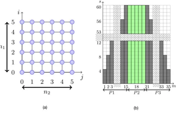
Let us consider a nanoparticle composed of 𝑛 × 𝑛 atoms on a 2D Cartesian grid as illustrated in the next figure.

In the following we consider both the geometry of the particle and the histogram which stores the densities of states 𝑧(𝑚, 𝑠, 𝑐).

Figure 2. (a) schematic 2D Cartesian particle grid. (b) Histogram for a 6x6 lattice.

In the particular case of a 𝑛 × 𝑛 grid, the operations of the above algorithm, can be scheduled by adding the atoms according to the topology of the grid, row by row. Then, at step (𝑖, 𝑗),

𝑖

rows are complete, and the

𝑖 +

st row contains 𝑗 atoms. The atoms to which further atoms will be attached are the 𝑛 atoms constituted by the 𝑗 atoms of the row currently

built, and the 𝑛 − 𝑗 last atoms of the previous row. Adding a new atom discards the atom below, to which no new node will be attached; this creates two new edges (except if 𝑗 = or 𝑖 = ) that can be balanced or not. 𝜎 can thus be coded as a vector of 𝑛 binary values (at most: for the first row, 𝜎 is incomplete).

With |𝐴| = 𝑛₁× 𝑛₂ , |𝐵| = (𝑛₁+ 𝑛₂− ) , |𝐿| = 𝑛₁(𝑛₂− ) + 𝑛₂(𝑛₁− ) , and 𝑙 = 𝑛2, the complexity of this algorithm is 𝛩((𝑛1𝑛2)3(𝑛1+ 𝑛2) 𝑛2) = 𝑂(𝑛

7

2 𝑛), taking

𝑛 = 𝑛₁𝑛₂ and choosing 𝑛 as the smallest dimension of the grid.

The algorithm below consists of loops over the geometry (𝑖, 𝑗) and histogram (𝑚, 𝑠, 𝑐) which are respectively illustrated in the two figures 2a and 2b.

We create three functions index_2D ( m, s, c ),

get_global_dependencies_2dCart_msc(k1D_deps, m, s, c), and

compute_2dCart_msc(z,k D-, z,k D_deps-, i, j, m, s, c). Those three functions are called in the inner loop c.

At each step it gets the data reference in histogram by calling index_2D(𝑚, 𝑠, 𝑐). It updates one line of index K1D, of the array 𝑧 considering the 8 dependencies. Indices of the dependencies are stored in the array K1D_deps and correspond to the triplet (𝑚, 𝑠 − , 𝑐), (𝑚, 𝑠 − , 𝑐), (𝑚 − , 𝑠, 𝑐), (𝑚 − , 𝑠 − , 𝑐), (𝑚 − , 𝑠 − , 𝑐), (𝑚 − , 𝑠 − , 𝑐 − ).

This array is updated at each step by calling the function get_global_dependencies_2dCart_msc(𝑘 𝐷_𝑑𝑒𝑝𝑠, 𝑚, 𝑠, 𝑐).

The update of the intermediate state is performed by

compute_2dCart_msc(𝑧,𝑘 𝐷-, 𝑧,𝑘 𝐷_𝑑𝑒𝑝𝑠-, 𝑖, 𝑗, 𝑚, 𝑠, 𝑐). It consists in a loop over 𝜎.

Algorithm: Dynamic programming for 2D cartesian grid

For = : ₁ For 𝑗 = : 𝑛₂ {𝑛 < 𝑛 } For 𝑚 = 𝑚𝑎𝑥𝑀: − : {(𝑖 + ) ∗ 𝑛 + 𝑗 + } For 𝑠 = 𝑠𝑚𝑎𝑥_𝑚: − : For 𝑐 = : 𝑐 <= 𝑚.and.𝑐 < 𝑛 + ∗ (𝑖 + ) 𝑘 𝐷 = 𝑖𝑛𝑑𝑒𝑥_ 𝐷(𝑚, 𝑠, 𝑐, 𝑛, 𝑠𝑖𝑧𝑒𝐶, 𝑠𝑚𝑎𝑥, 𝑠𝑖𝑧𝑒 𝐷) 𝑔𝑒𝑡_𝑔𝑙𝑜𝑏𝑎𝑙_𝑑𝑒𝑝𝑒𝑛𝑑𝑒𝑛𝑐𝑖𝑒𝑠_ 𝑑𝐶𝑎𝑟𝑡_𝑚𝑠𝑐(𝑘 𝐷_𝑑𝑒𝑝𝑠, 𝑚, 𝑠, 𝑐) 𝑐𝑜𝑚𝑝𝑢𝑡𝑒_ 𝑑𝐶𝑎𝑟𝑡_𝑚𝑠𝑐(𝑧,𝑘 𝐷-, 𝑧,𝑘 𝐷_𝑑𝑒𝑝𝑠-, 𝑖, 𝑗, 𝑚, 𝑠, 𝑐) EndFor EndFor EndFor EndFor EndFor

Complexity and experimental platform

In the t-loop of compute_2dCart_msc , the update consists in multiple reads in 𝑍,𝐾 𝐷_𝑑𝑒𝑝𝑠- array, and 𝑛 independent write in 𝑍,𝐾 𝐷-. We can exploit the later for a parallel loop implementation on a shared memory architecture.

The dynamic programming in the 2D case decreases dramatically the time complexity, but multiply the memory complexity by 𝑛 according to the study above. Nanoparticles of our interests corresponds to a range from 𝑛 = × to 𝑛 = × .

Let us assume that the frequency of a processor unit is about 2.6 GHz and a memory on a node is about 32 GB, we can illustrate this complexity given order of human perception.

The table below shows that, under those assumptions, we can now consider nanoparticle simulation from hours to days, and few weeks in the largest case with our approach.

The figure 3 shows the memory complexity function of the size of the problem for the dynamic programming approach. The complexity has increased and exhibit the needs of distributed memory architecture.

In this article simulation for grids of atoms up to × where performed on a single shared memory node with 16 cores.

Time complexity 𝑶 .𝒏72 𝒏/ for human perception

Problem size 6x6  14x14 15x15  17x17 18x18  19x19 20x20

Time order minutes hours days weeks

Figure 3. Memory complexity of the computation of the density of state for a 2D network; for

12

3. Numerical results and discussion

In a first stage, we look for the size effects on the thermal and the pressure behaviour of the HS fraction of a SCO nanoparticle. Next, we study the shape effects on the pressure behaviour of the thermal-dependence of the HS fraction. In each stage, we consider the two following alternatives: calculations with ligand-field 𝐿 and calculations without ligand-field.

In the present study, we will analyze the size and shape effects on the thermal and pressure dependence of the HS fraction for two typical spin-crossovers compounds characterized by a set of thermodynamic parameters (enthalpy and entropy changes). The first one (system 1) has /kB =1300K, ln(g) =6.01 leading to the transition temperature Teq=216 K and the second

one (system 2) is characterized by /kB =1978,6 K, ln(g) =6.9 (transition temperature

Teq=286 K).

3.1 2D size effects - The case L≠0

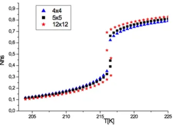
Figure 4 gives the temperature effect on the HS fraction for a given applied isotropic pressure when the interaction at the boundary of the SCO system with the surrounding medium cannot be neglected (𝐿 ≠ ). The analysis of the results obtained from 3

×

3, 4

×

4, 5

×

5 and 12

×

12 square lattices shows the presence of a thermal hysteresis with the smaller sizes, 3

×

3 and 4

×

4 squares compared to the larger 5

×

5, 12

×

12 which exhibit a gradual spin transition. In fact, when edge effects increase as a result of a higher perimeter to surface ratio, which is the case with the smaller squares compared to the larger ones, the transition temperature shifts to the reference edge temperature, 𝑇𝑒𝑞𝑠𝑢𝑟𝑓 = (𝛥 − 𝐿)/𝑘𝐵𝑙𝑛 𝑔. Because

hysteresis phenomenon is the fingerprint of first order transition, this result means that 𝑇_𝑒𝑞 must be lower than the critical temperature, 𝑇_𝐶, at which order-disorder transition of the corresponding Ising model occurs.

Parameter values are chosen from typical experimental data of standard SCO compounds and are fixed at: /kB =1300K, G/kB=172.2K, J/kB = 13.5 K, L/kB =130 K and ln(g) =6.01.

Using these values, we obtain for the curie temperature, TC = (2.269J +G)/kB=203 K, when

short range and long range interactions J and G are present and for the surface and bulk transition temperatures, 𝑇_𝑒𝑞𝑠𝑢𝑟𝑓= 7 K and 𝑇_𝑒𝑞𝑏𝑢𝑙𝑘= K, respectively. Compared to the curie temperature, the surface and bulk transition temperatures fulfill the following inequalities, 𝑇_𝑒𝑞𝑠𝑢𝑟𝑓< 𝑇_𝐶, whereas 𝑇_𝑒𝑞𝑏𝑢𝑙𝑘> 𝑇_𝐶. A gradual transition is obtained with the latter relation, while the former implies a thermal hysteresis for surface lattice. It means that decreasing the size of the nanoparticles favors the surface effects for which the conditions of appearance of a first-order transitions are fulfilled.

Figure 4. Thermal evolution of the HS fraction for different lattice sizes: 3x3 (green left

triangle), 4x4 (blue up triangle), 5x5 (black squares), 12x12 (red stars). The computational parameters are: Δ/kB = 1300 K, G/kB = 172.2 K, J/kB = 13.5 K, L/kB = 130 K, ln(g) = 6.01.

Concerning the effect of the pressure on the thermal properties of the SCO nanoparticules, we can see from Eq. (8) that the hydrostatic pressure appears as a conjugate parameter of temperature[41]. Increasing pressure stabilizes the LS state and it is equivalent to reducing the temperature.

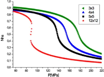
Figure 5 summarizes the pressure dependence of the HS fraction under isothermal conditions at T=300 K, for the several lattice sizes. It is noted, as expected, that strong (resp. weak) pressure values stabilize the LS (resp. HS) state. As a result, when hydrostatic pressure is increased the molecules changes from the HS to the LS state. Moreover, and in contrast with the thermal behaviors of Fig. 4, the increase of the system’s size leads to the increase of the width of the pressure hysteresis loop (12x12). It is observed that this isothermal transition depends on temperature, whose variation affects not only the width of the pressure hysteresis but also the character (first-order or gradual) of the transition.

Figure 5. Pressure-dependence of the HS fraction in isothermal conditions (T=300 K) for

different lattice sizes: 3x3 (green left triangle), 4x4 (blue up triangle), 5x5 (black squares), 12x12 (red stars). The computational parameters are: Δ/kB = 1978.6 K, G/kB = 172.2 K, J/kB =

48 K, L/kB = 130 K, ln(g) = 6.906, ΔV = 100 Å3.

- The case L=0

We now compare the thermal and pressure-dependences of the HS fraction when the interactions between the edges molecules and their surrounding environment are not taken

14

into account. First, we start with the case of thermal hysteresis of Fig. 4, for which we fix 𝐿 = . Hence, the effective ligand field becomes the same for surface and bulk atoms leading to a unique surface and bulk transition temperature, 𝑇 = K, as clearly depicted in Fig. 6.

Figure 6. Thermal evolution of the HS fraction for different lattice sizes: 4x4 (blue up

triangle), 5x5 (black squares), 12x12 (red stars). The computational parameters are: Δ/kB =

1300 K, G/kB = 172.2 K, J/kB = 16.8 K, L/kB = 0 K, ln(g) = 6.01.

The thermal behavior for the case L=0 is almost identical in the three numerical simulations: when the size increases the hysteresis width is increased and the equilibrium temperature is the same for the three cases. Indeed, according to Eqs. (7) and (8) the equilibrium temperature remains independent of the lattice size then L=0 (the system does not experience any surface effects). In contrast the order-disorder transition TOD increases with lattice size and then the

thermal hysteresis becomes wider (see Fig 3) when the lattice size increases.

When the surface effects are absent (L=0), when one applies an isotropic pressure, under isothermal conditions at T=300K, the results obtained of the pressure dependence of the HS fraction (see Fig. 7) are significantly different from those of Fig. 5. If one considers the lattices 5x5 and 12x12, we clearly see that their hysteresis widths are much wider than those of corresponding lattices of Fig. 5. For example, the lattice 12x12, exhibits in Fig. 7 a pressure hysteresis width given by ΔP ~ 13 MPa compared to 7 MPa for Fig. 5 and a pressure transition P1/2bulk = (kBTln(g)-Δ)/ΔV ~ 52 MPa, common to all other curves, which is smaller

Figure 7. Pressure-dependence of the HS fraction for T=300 K. for different lattice sizes: 4x4

(blue up triangle), 5x5 (black squares), 12x12 (red stars). The computational parameters are: Δ/kB = 1978.6 K, G/ kB = 172.2 K, J/ kB = 48, L/kB = 0 K and ln(g) = 6.906, ΔV = 100 Å3.

3.2 2D Shape effects under pressure

In a previous study, Guerroudj et al [35] analyzed the thermal-dependence of the HS fraction for different lattice shapes of SCO in nano configuration topology for a fixed total number of atoms (144). Here, we analyze the pressure-dependence of the HS fraction for different lattice shapes comprising 144 SCO molecules. We start with a 12x12 square lattice and through successive transformations from a square to a rectangle, one length is increased at the expense of the width sweeping all the different possible shapes until an elongated rectangular 2x72 lattice is obtained. For a × lattice, we define the aspect ratio parameter, = ( +

− )/ , as the ratio between surface and volume numbers of molecules. Thus, for a 12x12 square-shape, we calculate = . , while for rectangular-shaped lattices of size 9x16, 8x18, 6x24, 4x36, 3x48 and 2x72, we found the respective values, 0.32, 0.33, 0.39, 0.53, 0.68 and 1. Figure 8 shows two different shapes for a system of 144 molecules.

(a) (b)

Figure 8. (a) Square lattice with size 12x12 with a number core atoms 𝑁_𝐶 = and atoms at the edge, 𝑁_𝑒 = . (b) Rectangle-shaped lattice with size 4x36, containing 𝑁_𝐶= 8 core atoms and 𝑁𝑒= 7 edge sites. Black and red dots represent respectively the core (Nc) and the

edge (Ne) lattice sites.

- The case L≠0

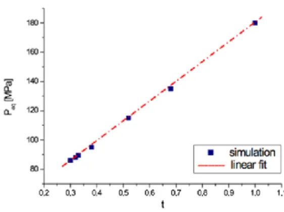
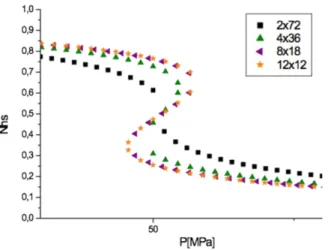
As shown in Fig. 9a, the 2x72 (t=1) and 3x48 (t=0.68) lattices exhibit a gradual thermal spin transition. A first-order transition with a hysteresis loop appears when the “t” value decreases. We note that the width of the loop increases when t decreases and seems to saturate for the lattices 8x18, 9x16 and 12x12. In addition, Fig. 9b reporting the behavior under pressure indicates that the transition pressure, defined as (Pup+Pdown)/2 which is approximately the

(a) (b)

Figure 9. (a) Evolution of the high spin versus the pressure for several shapes : 2x72 (black

square), 3x48 (red circle), 4x36 (green up triangle), 6x24 (blue down triangle), 8x18 (purple left triangle), 9x16 (dark yellow right triangle), 12x12 (orange star); the computational parameters are : Δ/kB = 1978.6 K, G/ kB = 172.2 K, J/kB = 49 K, L/kB = 120 K, T=300 K,

ln(g)=6.906, ΔV=100 Å3 ; (b) Zoom around the hysteresis-loop for the system shapes 8x18 (purple left triangle), 9x16 (dark yellow right triangle) and 12x12 (orange star).

Figure 10. The pressure transition 𝑃 versus the surface/volume parameter t.

- The case L=0

Figure 11 displays the pressure-dependence of the HS fraction for several lattice shapes in isothermal conditions (T=300 K). We observe that, except for the 2x72 (t=1) lattice which

exhibits a gradual spin transition between the HS and the LS state, all other systems present a hysteresis loop, typical of a first-order transition. The width of this hysteresis loop increases when t decreases. This behavior is in line with that of Fig. 9b, obtained for L=0. Moreover, one can also notice that the pressure transition, 𝑃 , in Fig.10 remains invariant (as in Fig. 10) whatever the shape of the material.

Figure 11. Evolution of the high spin versus the pressure for several shapes in isothermal

conditions (T=300 K) for, 2x72 (black square), 4x36 (green up triangle), 8x18 (purple left triangle), 12x12 (orange star) lattices. The computational parameters are : Δ/kB = 1978.6 K,

G/ kB = 172.2 K, J/kB = 49 K, L/kB = 120 K, ln(g)=6.906, ΔV = 100 Å3.

4. Summary and conclusion

In this paper, the computation of the Hamiltonian is based on the exact density of states, obtained by the algorithm presented in Section 2.2, and we analyze the behavior of 2D spin-crossover compounds under temperature and pressure. We focus on the effect of the interactions between nanoparticles at the edges and the matrix in their specific local environment, modelled with the coupling parameter, 𝐿. When 𝐿 = , the temperature and the pressure play as conjugate parameters, and both of them lead to thermal hysteresis as the size of the nanoparticle is increased. In contrast, when

𝐿 ≠

, opposite effects for the pressure and temperature are observed on the thermal hysteresis as function of the nanoparticle size. The main effect underlying these differences in the simulated behaviours is solely related to the relationship between the equilibrium temperature and the order-disorder temperature when 𝑔 = (unit degeneracy ratio) and 𝛥 = and 𝐿 =0 (absence of ligand field), i.e., mainly a temperature dependence. Indeed, the pressure effect is independent of L at all sizes except in the limit of very small lattices. This property is due to a concomitance of the unequal effect of pressure in the bulk and at the surface because of a weaker ligand field at the surface compared to that in the bulk and the surface/volume ratio effect which is parametrized by 𝑡. On the other hand, one can easily imagine that the effective short- and long-range interactions,J and 𝐺, which have an elastic origin, may depend on the applied pressure through the change of the lattice parameter and the bulk modulus under pressure. In addition, since the elastic and phonon properties of the surface and the bulk are different, additional

degrees of freedom may also emerge. For example, the effect of an expansion of the interaction parameters in terms of a reduced pressure parameter relative to a maximum pressure or in terms of a pressure law may be investigated in this respect for a deeper understanding of the SCO properties under various stimuli. This will benefit to the necessary reliability of new technological applications based on the switchable properties of these materials. Nevertheless, the results reported in this work are consistent with available experimental data as far as the effect of the internal interaction strength, the local environment at the surface or the system’s size on the thermal and pressure induced transitions are concerned.

Acknowledgments

The authors are grateful to Sallah E. Allal and Camille Harlé who did the preliminary simulations during their master internship. CHAIR Materials Simulation and Engineering of UVSQ-UPSAY, the French "Ministère de la Recherche", the Université de Versailles St. Quentin-en-Yvelines, Université Paris-Saclay, CNRS and ANR BISTA-MAT (ANR-12-BS07-0030-01) are warmly acknowledged for the financial support.

References

1. Coronado E., Nat. Rev. Mater (2019) doi:10.1038/s41578-019-0146-8

2. Gütlich P. and Goodwin H.A., Top. Curre. Chem. Spin Croosover in Transition Metal Compounds I-III, Springer, Heidelberg, Berin, 2004

3. Gütlich, P., Hauser, A. & Spiering, H.. Angew. Chem. Int. Ed. 33, 2024–2054 (1994).2

4. Köhler P.,Jakobi R., Meissner E., Wiehl L., Spiering H.and Gütlich P., J. Phys. and

Chem. of Solids, 1990, 51, 239-247].

5. Rotaru A., Dugay J., Tan R.P., Guralskiy I.A., Salmon L., Demont P., Carrey J., Molnar G., Respaud M., Bousseksou A., Adv. Mater. 2(, 1745-1749 (2013)

6. Peng, H.; Tricard, S.; Felix, G.; Molnar, G.; Nicolazzi, W.; Salmon, L.; Bousseksou, A. Angew. Chem. Int. Ed. Engl. 2014.

7. Jureschi C., Linares J., Boulmaali A., Dahoo P.R., Rotaru A. and Garcia Y., Sensors,16, 187, (2016)

8. Shepherd H.J., Gural’skiy I.A., Quintero C.M., Tricard S., Salmon L. Gabor G., Bousseksou A., Nat; Commun. 4, 2607 (2008)

9. Muraoka, A.; Boukheddaden, K.; Linares, J.; Varret, F, Phys. Rev. B 84, 054119 (2011)

10. Ahmed Slimani, Kamel Boukheddaden, François Varret, Hassane Oubouchou, Masamichi Nishino, and Seiji Miyashita, Phys. Rev. B 87, 014111, (2013)

11. Linares J, Jureschi C, Boukheddaden K, Magnetochemistry, 2, 24, (2016)

12. Boukheddaden K., Phys. Rev. B 88, 134105, (2013)

13. Nishino M. ,Boukheddaden K., and Miyashita S., Phys. Rev. B 79, 012409, (2009)

14. Klokishner S., Linares J., Varret F., Chemical. Physics, 255, 317-323, (2000)

15. Morscheidt W, Jeftic J, Codjovi E, Linares J, Bousseksou A, Constant-Machado H, Varret F, Meas. Sci.Techn., 9, 1311-1315, (1998)

16. Rotaru A, Varret F, Gîndulescu A, Linares J, Stancu A, Létard JF, Forestier T, Etrillard C, Eur. Phys. J. B 84, 439-449, (2011)

17. Jeftic J, Menéndez N, Wack A, Codjovi E, Linarès J, Goujon A, Hamel G, Klotz S, Syfosse G, Varret F , Meas. Sci. Techn., 10, 1059-1064, (1999)

18. Bousseksou, A.; Boukheddaden, K.; Goiran, M.; Consejo, C.; Boillot, M.L.; Tuchagues, J.P., Phys. Rev. B, 65 (2002)

19. Decurtins, S.; Gutlich, P.; Kohler, C.P.; Spiering, H.; Hauser, Chem. Phys. Lett. 1984, 105, 1–4

20. Coronado E., Galan-Mascaros J.R., Monrabal-Capilla M., Garcia-Martinez J., Pardo-Ibanez P., Adv. Mater. 19, 1359-1361 (2007)

21. Volatron F., Catala L., Riviere E., Gloter A., Stephan O., Mallah T., Inorg. Chem. 47, 6584-6586 (2008)

22. Catala L., Volatron F., Brinzei D., Mallah T., Inorg. Chem. 48, 3360-3370 (2009)

23. Wajnflasz J, Pick R, J. Phys.Colloques, 32, 91-92, (1971)

24. Bousseksou A, Nasser J, Linares J, Boukheddaden K, Varret F, J. Physique I 2 1381, (1992)

25. Linares J., Spiering H., Varret F., Eur. Phys. J. B, 10, 271-275 (1992).

26. Shteto I., Linares J., Varret F., Physical Review E 56, 5128-5137, (1997)

27. Nasser J., Boukheddaden,K. Linares J., Eur. Phys. J. B 39, 219 (2004).

28. Enachescu C., Nishino M., Miyashita S., Stoleriu L.,Stancu A., Physical Review B 86, 054114 (2012).

30. K. Affesa, A. Slimani, A. Maaleja, K. Boukheddaden, Chemical Physics Letters, 718 (2019) 46-53

31. D’Avino G. Painelli A., Boukheddaden K., Phys. Rev. B, 2011, 84, 104119 32. Biernacki S. W., Clerjaud B., Phys. Rev. B 2005, 72, 024406

33. Enachescu C., Stoleriu L., Nishino M., Miyashita S., Stancu A., Lorenc A., Bertoni R., Cailleau H., Collet E., Phys. Rev. B 95, 224107 (2017)

34. Linares J, Jureschi C, Boulmaali A, Boukheddaden K, Physica B, 486, 164–168, (2016)

35. Guerroudj S., Caballero R., De Zela F., Jureschi C.,Linares J.. Boukheddaden,K. J. Phys. : Conf. Ser.738 (2016) 012052.

31 Harlé C., Allal S. E., Sohier D., Dufaud T., Caballero R., de Zela F., Dahoo P.-R., Boukheddaden K., LinaresJ., Journal of Physics: Conference Series, IOP Publishing, 2017, 936, pp.012061. ⟨10.1088/1742-6596/936/1/012061⟩

32 Kim, S.Y, Journal of Physical and Mathematical Sciences 5(11), 1684-1689 (2011) 33 Bellman, R.: Dynamic Programming. Princeton University Press, Princeton, NJ,

USA, 1 edn. (1957)

34 Stosc B., Milosevic S. Stanley H.E.,Phys. Rev. B 41, 11466-11478 (Jun 1990) 35 Allal, S.E., Harle, C., Sohier, D., Dufaud, T., Dahoo, P.R., Linares, J, European

Journal of Inorganic Chemistry 2017(36), 4196{4201 (2017)

36 Boukheddaden K., Ritti M.H., Bouchez G., Sy M., Dirtu M.M., Parlier M., Linares J., Garcia Y., J. Phys. Chem. C 2018, 122, 7597−7604