HAL Id: hal-00496618
https://hal.archives-ouvertes.fr/hal-00496618
Submitted on 30 Jun 2010HAL is a multi-disciplinary open access
archive for the deposit and dissemination of sci-entific research documents, whether they are pub-lished or not. The documents may come from
L’archive ouverte pluridisciplinaire HAL, est destinée au dépôt et à la diffusion de documents scientifiques de niveau recherche, publiés ou non, émanant des établissements d’enseignement et de
Modelling fish population movements: from an
individual-based representation to an advection-diffusion
equation
Blaise Faugeras, Olivier Maury
To cite this version:
Blaise Faugeras, Olivier Maury. Modelling fish population movements: from an individual-based representation to an advection-diffusion equation. Journal of Theoretical Biology, Elsevier, 2007, 247, pp.837-848. �hal-00496618�
Modelling fish population movements:
from an individual-based representation to an
advection-diffusion equation
Blaise Faugeras ∗ and Olivier Maury
IRD, UR 109 THETIS,
CRH, Avenue Jean Monnet, B.P. 171, 34203, S`ete cedex, France
Abstract
In this paper we address the problem of modelling fish population movements. We first consider a description of movements at the level of individuals. An individual-based model is formulated as a biased random walk model in which the velocity of each fish has both a deterministic and a stochastic component. These compo-nents are function of a habitat suitability index, h, and its spatial gradient ∇h. We derive an advection-diffusion partial differential equation which approximates this individual-based model. The approximation process enables us to obtain a mecha-nistic representation of the advection and diffusion coefficients which improves the heuristic approaches of former studies. Advection and diffusion are linked and ex-hibit antagonistic behaviors: strong advection goes with weak diffusion leading to a directed movement of fish. On the contrary weak advection goes with strong dif-fusion corresponding to a searching behavior. Simulations are conducted for both models which are compared by computing spatial statistics. It is shown that the partial differential equation model is a good approximation to the individual-based model.
Key words: population dynamics, biased random walk, individual-based model, partial differential equation
1 Introduction
Population dynamics models are essential to help to understand marine ecosys-tems dynamics and to provide assessment of fish abundance and fishery
ex-∗ Corresponding author:
ploitation level. This is particularly true in the case of tuna fisheries, which are among the most valuable in the world and subject to increasing fishing pressure and to the effects of climate change. Although fish are mobile, models of population dynamics without any or with very crude representation of space are most of the time used for fisheries stock assessments. However, in order to understand the reasons and consequences of resource variability, many recent studies of ecological dynamics have emphasized the necessity to develop and use spatially explicit approaches.
Fish population dynamics can be represented with such partial differential equations (PDE). Spatial advection-diffusion models have a long history in ecology (e.g. Skellam, 1951; Okubo, 1980; Holmes et al., 1994), but their use in fishery science has grown recently, particularly for tuna population modelling purposes (Bertignac et al., 1998; Maury and Gascuel, 1999; Sibert et al., 1999; Lehodey et al., 2003; Faugeras and Maury, 2005). Among the difficulties which arise with such models an important one is the choice that has to be made to express the time and space dependent advection and diffusion coefficients.
A first approach, used by Sibert et al. (1999), is to set these parameters to be constant over large spatial regions and temporal seasons and to try to es-timate them by minimizing a cost function describing the distance between the outputs of the model and the available data. This is not completely satis-fying since the spatio-temporal variability of advection and diffusion terms is roughly represented.
A second approach followed for instance by Bertignac et al. (1998) and Faugeras and Maury (2005) is to parameterize advection and diffusion terms as func-tions of an habitat suitability index. This approach has the advantage to fully take into account the spatio-temporal variability of the habitat of a fish popu-lation with a small number of parameters. However its main drawback is that the expressions chosen to parameterize advection and diffusion coefficients are arbitrary. The advection field V is usually considered to be proportional to the spatial gradient of the habitat suitability index h : V = c∇h. The coeffi-cient c is the taxis coefficoeffi-cient. It determines the rate of movements of fish up gradients of the habitat suitability index. This coefficient can be a constant (Bertignac et al., 1998; Maury, 2000), or a simple and empirical function of h and ∇h (Faugeras and Maury, 2005). The diffusion matrix is always supposed to be diagonal. Its diagonal elements are either assumed to be constant or simple arbitrary functions of h.
In this paper we provide a mechanistic approach to derive an advection-diffusion fish population dynamics model from individual fish behavior. Our approach is based on a biased random walk model. This type of model can also be viewed as simple individual-based models (IBM). Such models are useful to describe movements at the level of individuals but cannot be easily
used to treat large populations. Instead some level of approximation has to be made to reduce the problem to a state equation in which the variable is the spatial density of individuals. Related works, concerning the transforma-tion of an individual-based or microscopic modelling into a populatransforma-tion-based or macroscopic modelling, are Alt (1980) and Gr¨unbaum (1999) in which the authors show that the solutions of an underlying differential-integral equation describing the movements of animals satisfy, under suitable assumptions, an advection diffusion equation. One can also be interested in Flierl et al. (1999) where the authors analyse the processes by which organisms form groups and discuss the transformation of IBM into continuum models. In the present study, an advection-diffusion equation is obtained as a truncated Kramers-Moyall cumulant expansion (Risken, 1996) of the spatial density function of individuals. The parameters of the IBM are used in the expressions of the ad-vection and diffusion terms. A consistent behavior is obtained concerning the dependence of these two terms on h and ∇h, and the balance between them. Advection and diffusion both are decreasing functions of the habitat index h. Moreover their dependence on ∇h implies that strong advection goes with weak diffusion leading to a directed movement of fish. On the contrary weak advection goes with strong diffusion corresponding to a searching behavior. This formalizes the heuristic approach of Faugeras and Maury (2005).
The paper is structured as follows. In Section 2 we describe the random walk model. It is viewed as a simple IBM and simulations are conducted in Section 4. In Section 3, starting from the random walk, a recursion equation is formulated for the spatial density of individuals. This equation is expanded with respect to two small parameters and finally approximated to give the advection-diffusion equation. Section 4 provides numerical simulations of both the IBM and PDE model. Spatial statistics are computed in order to compare the models. It is shown that the PDE model is a good approximation of the IBM despite of the simplifying assumptions that are made to derive the PDE model. The paper ends with a Conclusion section and two Annexes.
2 Individual-based model
In this Section we propose an individual-based model describing movements of n independent but identical fish. We assume that there is no interaction between individuals and that more than one individual can occupy a given position. Only horizontal movements are modelled and individuals evolve in a domain Ω ∈ R2 during a period of time [0, T ]. Oceanographic currents are not considered in this paper where flow effects are not taken into account. The modelling focusses on the biological processes which drive individual move-ments. It is assumed that individuals assess their environment and that the decisions they make concerning their movements depend on an habitat
suit-ability index function
h: R2
× [0, T ] → [0, 1]
The function h is supposed to synthesize all the informations (water temper-ature, forage concentration and dissolved oxygen concentration for example) that individuals take into account to adjust the direction and velocity of their displacements. Individuals are assumed to search for and stay in regions cor-responding to a high habitat suitability index. Therefore their movements are considered to be induced by their need to maximize h.
Each individual is characterized by its position x and has a velocity
v= vd
The norm, v, of the velocity is assumed to be deterministic whereas d is a stochastic unit-norm direction vector. An individual trajectory follows
dx dt = v
This equation is discretized using the explicit Euler method, assuming there exists a small mean time, τ , during which the velocity vector of an individual is constant. Therefore an individual positioned at x at time t will move to x+ v(x, t)τ at time t + τ .
The behavior of each individual is governed by the habitat suitability index h and its gradient ∇h. A simple linear relation is assumed between the norm of the velocity and the habitat suitability index
v(x, t) = v0(1 − h(x, t)) (1) where v0 is the maximum speed that a fish can reach. Hence fish located in regions where h is low have a higher velocity than those in regions where h is large.
The direction vector is given by
d= cos θ sin θ (2)
The angle θ is a realization of a random variable Θ which follows a von Mises distribution, g defined by
g(θ, κ, θ0) = 1
2πI0(κ)exp(κ cos(θ − θ0))
where I0 is the modified Bessel function of the first kind and of order 0 (see Appendix A). The distribution is centered around the mean angle θ0 = θ∇h ∈
] − π, π] given by the direction of the gradient ∇h (see Figure 1) and with a concentration parameter κ = α||∇h|| proportional to the norm of the gradient. Hence, at time t, the angle of displacement of a fish located at x is drawn from the probability density
f(θ, x, t) = g(θ, α||∇h(x, t)||, θ∇h(x, t))
= 1
2πI0(α||∇h(x, t)||)exp(α||∇h(x, t)|| cos(θ − θ∇h(x, t))
(3) ∇ h θ∇ h x y +π −π
Fig. 1. The unit circle, ∇h and θ∇h∈] − π, π].
Since the mean movement direction is given by the direction of the gradient ∇h, fish tend to maximize the habitat suitability index h. The concentration parameter is proportional to ||∇h|| and therefore high values of ||∇h|| induce direction vectors that strongly follow the direction of the gradient, correspond-ing to a directed movement behavior. On the contrary low values of ||∇h|| lead to less correlation between the direction vector and ||∇h||. This corresponds to a searching behavior.
3 Approximation of the IBM: advection-diffusion equation
In this Section, starting from the microscopic description of movements given by the IBM we formally derive a simplified macroscopic description in terms of an advection-diffusion partial differential equation.
In order to achieve this task we have to use approximating hypothesis. The first one is to consider in a first step that the norm v of the velocity vector for each individual is a constant, that is to say independent of time and space. As a consequence we can suppose that at each time step τ an individual moves a distance δ in a direction θ with a probability which depends on space and time through the density f (θ, x, t) of Eq. (3). The microscopic space and time
scale parameters, δ and τ , are considered to be small with respect to the macroscopic space and time scales defined by the dimensions of the spatial domain Ω and the time domain (0, T ).
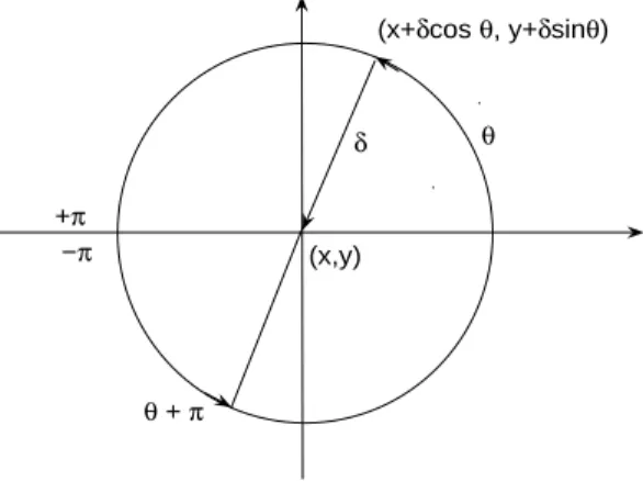
All individuals that can possibly reach position x = (x, y) at time t + τ lie at time t on a circle of radius δ centered on (x, y)(see Fig. 2). The density of individuals, p(x, y, t+τ ) at position (x, y) and time t+τ can thus be expressed with the following recursion:
p(x, y, t + τ ) =
Z π
−πp(x + δ cos θ, y + δ sin θ, t)f (θ + π, x + δ cos θ, y + δ sin θ, t)dθ =
Z π
−πp(x − δ cos θ, y − δ sin θ, t)f(θ, x − δ cos θ, y − δ sin θ, t)dθ
(4) θ (x,y) +π −π δ θ + π (x+δcos θ, y+δsinθ)
Fig. 2. All individuals that can possibly reach position (x, y) at time t + τ lie at time t on a circle of radius δ centered on (x, y).
The remaining part of the derivation of the desired advection-diffusion equa-tion from Eq. (4) relies on analytical computaequa-tions which are fully detailed in Appendix B. It is based first of all on second order Taylor expansions with re-spect to the space variables for the right hand side of Eq. (4) and with rere-spect to the time variable for the left hand side. Secondly the expansions are com-bined using recursive substitution and truncated neglecting high order terms. The results concerning the moments of the von Mises distribution given in Appendix A enable us to define a, b, c, d and e in the following way:
a = Z π −πf(θ, x, y, t) cos θdθ = I1(α||∇h(x, t)||) I0(α||∇h(x, t)||)cos θ∇h(x, t), b = Z π −πf(θ, x, y, t) sin θdθ = I1(α||∇h(x, t)||) I0(α||∇h(x, t)||)sin θ∇h(x, t),
c= Z π −πf(θ, x, y, t) cos 2 θdθ= 1 2(1 + I2(α||∇h(x, t)||) I0(α||∇h(x, t)||)cos 2θ∇h(x, t)), d= Z π −πf(θ, x, y, t) sin θ cos θdθ = 1 2 I2(α||∇h(x, t)||) I0(α||∇h(x, t)||)sin 2θ∇h(x, t), e= Z π −πf(θ, x, y, t) sin 2 θdθ= 1 2(1 − I2(α||∇h(x, t)||) I0(α||∇h(x, t)||)cos 2θ∇h(x, t)). Eventually this leads to approximate Eq. (4) by the following advection-diffusion PDE: ∂tp= −[∂x( δ τap) + ∂y( δ τbp)] +[∂x(δ 2 2τ(c − a 2 )∂xp) + ∂x(δ 2 2τ(d − ab)∂yp) +∂y(δ 2 2τ(d − ab)∂xp) + ∂y( δ2 2τ(e − b 2 )∂yp)] (5)
Now, as was the case in the IBM, we assume that δ is not a constant but satisfies
δ
τ = v0(1 − h) and hence we also have that
δ2 2τ =
τ
2(v0(1 − h)) 2
Finally defining the advection velocity
V = v0(1 − h) a b = v0(1 − h)I1(α||∇h||) I0(α||∇h||) cos θ∇h sin θ∇h (6)
and the diffusion matrix D = τ 2(v0(1 − h)) 2 c− a2 d − ab d− ab e − b2 = τ 2(v0(1 − h)) 2 × {12(1 − I2I0(α||∇h||) (α||∇h||)) 1 0 0 1 +[I2(α||∇h||) I0(α||∇h||) − ( I1(α||∇h||) I0(α||∇h||)) 2 ] cos2θ∇ h sin θ∇hcos θ∇h sin θ∇hcos θ∇h sin2θ∇h
}
(7)
we obtain the final advection-diffusion equation approximating the IBM:
∂tp= ∇ · (D∇p − Vp) (8) Note that the diffusion matrix, D has non zero off diagonal terms and its elements are the centered second order trigonometric moments of the von Mises distribution. D is also symetric positive.
The advection velocity V is of chemotaxis type. It is oriented in the direction of ∇h and its amplitude is modulated by I1I0(α||∇h||)
(α||∇h||) an increasing function of ||∇h||. At a given level of habitat suitability index h, the balance between advection and diffusion only depends on the gradient ||∇h||. Strong gradients impose strong advection and weak diffusion whereas weak gradients induce weak advection and strong diffusion.
4 Numerical simulations and comparisons of the models
The IBM proposed in Section 2 is approximated by an advection-diffusion equation derived in Section 3. In this section we conduct numerical simulations for both models and compute some spatial statistics in order to compare them.
An algorithm to simulate the IBM described in Section 2 is not difficult to program. We consider a rectangular spatial domain Ω = (0, Lx) × (0, Ly) large enough for individuals never to reach its boundaries during the period of the simulation of length T = Kτ . For the sake of simplification we consider a time independent habitat suitability index h defined on Ω. As initial condition a set of n = 104 individuals are positioned at the same location: x0
i = x0, i = 1...n. At each time step (denoted by k), of length τ , and for each point
xki, h(xk
i) and ∇h(xki) are computed, and an angle θik is drawn from the von Mises distribution. Each individual then moves according to
xk+1i = xki + v0(1 − h(xki))τ cos θk i sin θk i
All experiments were conducted with τ = 10−1 and v0 = 1. The IBM simu-lation algorithm was programmed with Matlab. In order to generate random numbers from a von Mises distribution we used a Matlab code developed by A. Bar-Guy and A. Podgaetsky available on Matlab central website. It imple-ments the method suggested in Yuan and Kalbleisch (2000) and described in Devroye (2002).
In the approximation procedure of the PDE model a finite difference dis-cretization is used. Equation (8) is solved on a grid with a spatial resolution of ∆x = ∆y = 10−2
and a discrete time step ∆t = 10−2
is used. Since Ω is bounded, boundary conditions need to be added to Eq. (8). We have used Neumann boundary conditions. In order to be consistent with the simulation of the IBM we consider the following initial condition
p0 = n ∆x∆yδx0
The numerical scheme implemented is based on a splitting method (Strang, 1968; Marchuk, 1990). Diagonal diffusion terms are treated implicitly in time whereas off diagonal diffusion terms are treated explicitly. Concerning advec-tion terms, the MUSCL scheme (monotonic upstream centered scheme for con-servation laws (Van Leer, 1977)) is used. The choice of the advection scheme has an important part in the spatial statistics computed from the solution of the PDE model. The numerical diffusion introduced into the solution of the PDE by the use of a simple upwind or centered difference advection scheme leads to unreliable computed variances. The MUSCL scheme is more compli-cated to implement but far less diffusive.
In order to compare the population distributions generated by the IBM on the one hand and by the PDE approximating model on the other, we compute the first three centered spatial moments as functions of time For the PDE model the mean x position is computed as
mx,P DE(t) = Z Ωxp(x, y, t)dxdy Z Ωp(x, y, t)dxdy (9)
and for the IBM model it is computed as mx,IBM(t) = 1 n n X i=1 xi(t) (10)
The variance about the mean x position is
σx,P DE2 (t) = Z Ω(x − mx,P DE(t)) 2 p(x, y, t)dxdy Z Ωp(x, y, t)dxdy (11)
for the PDE and
σx,IBM2 (t) = 1 n− 1 n X i=1 (xi(t) − mx,IBM(t))2 (12) for the IBM. Finally the third standardized centered moment or skewness in x is computed as γx,P DE(t) = Z Ω(x − mx,P DE(t)) 3 p(x, y, t)dxdy σ3 x,P DE(t) Z Ωp(x, y, t)dxdy (13)
for the PDE and as
γx,IBM(t) =
q
n(n − 1) n− 2
√nPn
i=1(xi(t) − mx,IBM(t))3 (Pn
i=1(xi(t) − mx,IBM(t))2)3/2
(14)
Similar formulas are used to compute moments in the y direction.
4.1 Experiments 1 and 2
Both models are run on a time interval of length T = 2 and on a spatial domain Ω = (0, 2) × (0, 2). The initial position of all individuals is x0 = (0.6, 1). The habitat suitability index function is h(x, y, t) = x
2 and therefore the gradient is oriented along the x-axis. The only difference between both experiments is the value of the concentration parameter, α = 5 in experiment 1 and α = 1 in experiment 2.
Figures 3 and 7 show the solutions of both models at T = 2. Due to the different values of the concentration parameter individuals are more scattered in experiment 2 than in experiment 1. As a consequence, advection in the direction of the gradient ∇h is stronger in experiment 1 than in experiment 2.
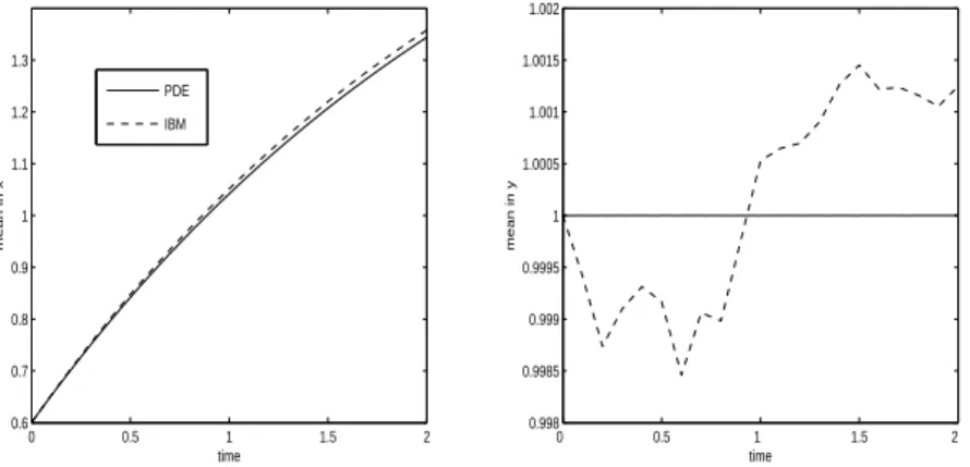
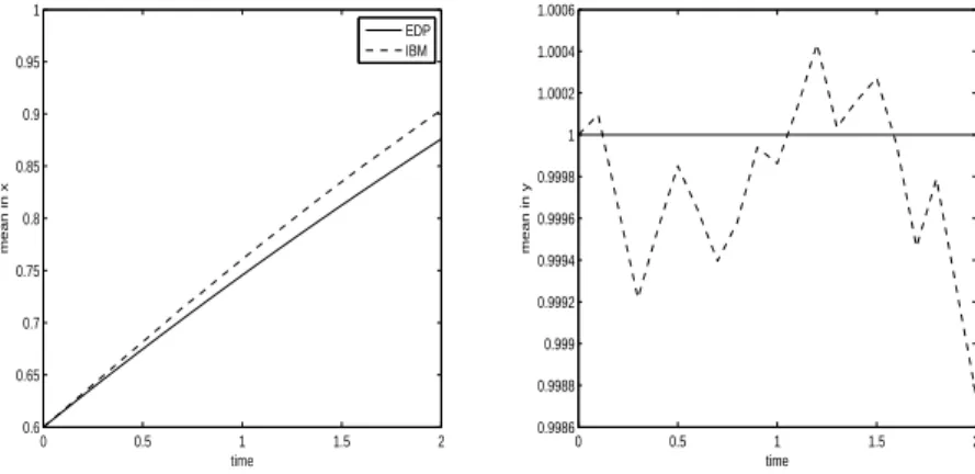
The mean positions, mx,P DE, mx,IBM and my,P DE, my,IBM are plotted on Figure 4 as functions of time for experiment 1. The solution of the PDE model appears to follow closely the solution of the IBM. This is also true for experiment 2 as shown on Figure 8 although, because of a strongest diffusion, the difference between mx,P DE, mx,IBM at final time is highest in experiment 2 than in experiment 1.
The same type of conclusion, that is to say the solution of the PDE model follows closely the solution of the IBM, remains true for the second order centered moments as shown in Figures 5 and 9. This is not surprising since in the PDE approximation of the IBM (described in Section 3) second order derivative terms are taken into account (although some of them are neglected).
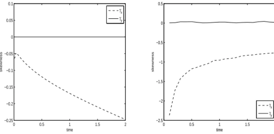
As could be expected the numerical results for the third order moments, or skewness, show much less correlation between the PDE model and the IBM (Figs. 6 and 10) than for the first two moments. Nethertheless some features of the IBM still appear in the PDE solution. In probability theory and statistics, skewness is a measure of the asymmetry of the probability distribution of a real-valued random variable. A distribution has positive skew (right-skewed) if the right (higher value) tail is longer or fatter and negative skew (left-skewed) if the left (lower value) tail is longer or fatter. In both experiments the skewness in the y direction, γy, is null for both the IBM and the PDE, indicating that the distribution is symmetrical about the x-axis. Although values are different the skewness in the x direction, γx, is negative for both the IBM and the PDE indicating that the distributions have a longer ”left” tail. This tail reflects the possibility for an individual not to move at each time step in the direction of the gradient with some probability depending on α. This probability is higher in experiment 2 than in experiment 1 and therefore the tail is bigger in experiment2 than in experiment 1.
4.2 Experiment 3
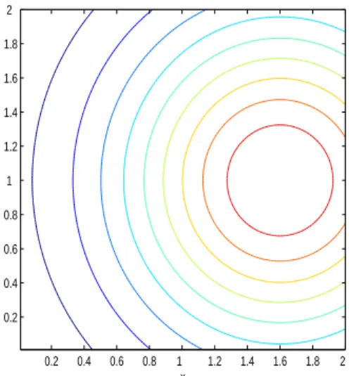
In this experiment the habitat suitability function is (see Fig. 11)
h(x, y, t) = exp(−((x − 1.6)2+ (y − 1)2))
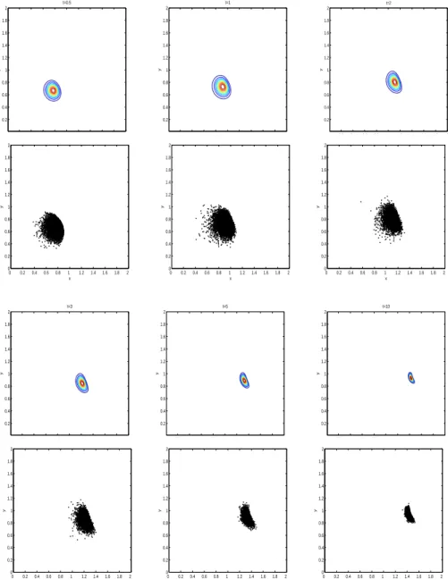
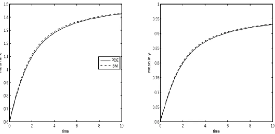
The initial position of all individuals is x0 = (0.6, 0.6) and the concentration parameter is α = 2. Figure 12 shows the time evolution of the solution for both the PDE model and the IBM. This experiment illustrates the effect of non-zero off-diagonal terms in the diffusion matrix. The solution of the PDE model is not symmetrical with respect to the x or y axis. Figures 13, 14 and 15 show the time evolution of the first three moments for both the PDE model and the IBM. As for experiments 1 and 2 the first two moments of the solution of the approximated PDE model closely follow those of the IBM. Differences
appear in the computation of the third moment. x y 0.2 0.4 0.6 0.8 1 1.2 1.4 1.6 1.8 2 0.2 0.4 0.6 0.8 1 1.2 1.4 1.6 1.8 2 0 0.2 0.4 0.6 0.8 1 1.2 1.4 1.6 1.8 2 0 0.2 0.4 0.6 0.8 1 1.2 1.4 1.6 1.8 2 x y
Fig. 3. Solution of the PDE model (left) and of the IBM (right) at final time T = 2 for experiment 1. The spatial domain is defined by Ω = (0, 2) × (0, 2). The habitat suitability index function is h(x, y, t) = x
2. The initial position of all individuals is x0= (0.6, 1). The concentration parameter is α = 5.
0 0.5 1 1.5 2 0.6 0.7 0.8 0.9 1 1.1 1.2 1.3 time mean in x PDE IBM 0 0.5 1 1.5 2 0.998 0.9985 0.999 0.9995 1 1.0005 1.001 1.0015 1.002 time mean in y
Fig. 4. Experiment 1. Mean position in x, mx,P DE(t) for the PDE model and
mx,IBM(t) for the IBM (left) and mean position in y, my,P DE(t) for the PDE and
0 0.5 1 1.5 2 0 0.5 1 1.5 2 2.5 3x 10 −3 time variance in x 0 0.5 1 1.5 2 0 0.002 0.004 0.006 0.008 0.01 0.012 0.014 0.016 time variance in y
Fig. 5. Experiment 1. Variance in x, σ2
x,P DE(t) for the PDE model and σ2x,IBM(t)
for the IBM (left) and variance in y, σ2
y,P DE(t) for the PDE and σ 2
y,IBM(t) for the
IBM (right). 0 0.5 1 1.5 2 −0.25 −0.2 −0.15 −0.1 −0.05 0 0.05 0.1 time skewness γx γy 0 0.5 1 1.5 2 −2.5 −2 −1.5 −1 −0.5 0 0.5 time skewness γx γy
Fig. 6. Experiment 1. Skewness in x and y for the PDE model (left) and for the IBM (right). x y 0.2 0.4 0.6 0.8 1 1.2 1.4 1.6 1.8 2 0.2 0.4 0.6 0.8 1 1.2 1.4 1.6 1.8 2 0 0.2 0.4 0.6 0.8 1 1.2 1.4 1.6 1.8 2 0 0.2 0.4 0.6 0.8 1 1.2 1.4 1.6 1.8 2 x y
Fig. 7. Solution of the PDE model (left) and of the IBM (right) at final time T = 2 for experiment 2. The spatial domain is defined by Ω = (0, 2) × (0, 2). The habitat suitability index function is h(x, y, t) = x
2. The initial position of all individuals is x0= (0.6, 1). The concentration parameter is α = 1.
0 0.5 1 1.5 2 0.6 0.65 0.7 0.75 0.8 0.85 0.9 0.95 1 time mean in x EDP IBM 0 0.5 1 1.5 2 0.9986 0.9988 0.999 0.9992 0.9994 0.9996 0.9998 1 1.0002 1.0004 1.0006 time mean in y
Fig. 8. Experiment 2. Mean position in x, mx,P DE(t) for the PDE model and
mx,IBM(t) for the IBM (left) and mean position in y, my,P DE(t) for the PDE and
my,IBM(t) for the IBM (right).
0 0.5 1 1.5 2 0 0.005 0.01 0.015 0.02 0.025 0.03 time variance in x 0 0.5 1 1.5 2 0 0.005 0.01 0.015 0.02 0.025 0.03 0.035 0.04 time variance in y
Fig. 9. Experiment 2. Variance in x, σ2
x,P DE(t) for the PDE model and σ2x,IBM(t)
for the IBM (left) and variance in y, σ2
y,P DE(t) for the PDE and σy,IBM2 (t) for the
IBM (right). 0 0.5 1 1.5 2 −0.5 −0.4 −0.3 −0.2 −0.1 0 0.1 0.2 time skewness γx γy 0 0.5 1 1.5 2 −0.6 −0.5 −0.4 −0.3 −0.2 −0.1 0 0.1 time skewness γx γy
Fig. 10. Experiment 2. Skewness in x and y for the PDE model (left) and for the IBM (right).
x y 0.2 0.4 0.6 0.8 1 1.2 1.4 1.6 1.8 2 0.2 0.4 0.6 0.8 1 1.2 1.4 1.6 1.8 2
Fig. 11. Experiment 3. Contour plot of the habitat suitability index function h(x, y) = exp(−((x − 1.6)2+ (y − 1)2)).
x y t=0.5 0.2 0.4 0.6 0.8 1 1.2 1.4 1.6 1.8 2 0.2 0.4 0.6 0.8 1 1.2 1.4 1.6 1.8 2 x y t=1 0.2 0.4 0.6 0.8 1 1.2 1.4 1.6 1.8 2 0.2 0.4 0.6 0.8 1 1.2 1.4 1.6 1.8 2 x y t=2 0.2 0.4 0.6 0.8 1 1.2 1.4 1.6 1.8 2 0.2 0.4 0.6 0.8 1 1.2 1.4 1.6 1.8 2 0 0.2 0.4 0.6 0.8 1 1.2 1.4 1.6 1.8 2 0 0.2 0.4 0.6 0.8 1 1.2 1.4 1.6 1.8 2 x y 0 0.2 0.4 0.6 0.8 1 1.2 1.4 1.6 1.8 2 0 0.2 0.4 0.6 0.8 1 1.2 1.4 1.6 1.8 2 x y 0 0.2 0.4 0.6 0.8 1 1.2 1.4 1.6 1.8 2 0 0.2 0.4 0.6 0.8 1 1.2 1.4 1.6 1.8 2 x y x y t=3 0.2 0.4 0.6 0.8 1 1.2 1.4 1.6 1.8 2 0.2 0.4 0.6 0.8 1 1.2 1.4 1.6 1.8 2 x y t=5 0.2 0.4 0.6 0.8 1 1.2 1.4 1.6 1.8 2 0.2 0.4 0.6 0.8 1 1.2 1.4 1.6 1.8 2 x y t=10 0.2 0.4 0.6 0.8 1 1.2 1.4 1.6 1.8 2 0.2 0.4 0.6 0.8 1 1.2 1.4 1.6 1.8 2 0 0.2 0.4 0.6 0.8 1 1.2 1.4 1.6 1.8 2 0 0.2 0.4 0.6 0.8 1 1.2 1.4 1.6 1.8 2 x y 0 0.2 0.4 0.6 0.8 1 1.2 1.4 1.6 1.8 2 0 0.2 0.4 0.6 0.8 1 1.2 1.4 1.6 1.8 2 x y 0 0.2 0.4 0.6 0.8 1 1.2 1.4 1.6 1.8 2 0 0.2 0.4 0.6 0.8 1 1.2 1.4 1.6 1.8 2 x y
Fig. 12. Solution of the PDE model (row 1 and 3) and of the IBM (row 2 and 4) at time t = 0.5, t = 1, t = 2, t = 3, t = 5 and final time T = 10 for experiment 3. The spatial domain is defined by Ω = (0, 2) × (0, 2). The habitat suitability index function is h(x, y, t) = exp(−((x−1.6)2
+(y −1)2)) (see Fig. 11). The initial position
0 2 4 6 8 10 0.6 0.7 0.8 0.9 1 1.1 1.2 1.3 1.4 1.5 time mean in x PDE IBM 0 2 4 6 8 10 0.6 0.65 0.7 0.75 0.8 0.85 0.9 0.95 1 time mean in y
Fig. 13. Experiment 3. Mean position in x, mx,P DE(t) for the PDE model and
mx,IBM(t) for the IBM (left) and mean position in y, my,P DE(t) for the PDE and
my,IBM(t) for the IBM (right).
0 2 4 6 8 10 0 1 2 3 4 5 6 7x 10 −3 time variance in x 0 2 4 6 8 10 0 1 2 3 4 5 6 7 8 9x 10 −3 time variance in y
Fig. 14. Experiment 3. Variance in x, σ2
x,P DE(t) for the PDE model and σ2x,IBM(t)
for the IBM (left) and variance in y, σ2
y,P DE(t) for the PDE and σy,IBM2 (t) for the
IBM (right). 0 2 4 6 8 10 −0.6 −0.5 −0.4 −0.3 −0.2 −0.1 0 0.1 0.2 0.3 time skewness γx γy 0 2 4 6 8 10 −1.4 −1.2 −1 −0.8 −0.6 −0.4 −0.2 0 0.2 0.4 time skewness γx γy
Fig. 15. Experiment 3. Skewness in x and y for the PDE model (left) and for the IBM (right).
5 Conclusion
In this paper we provide a mechanistic approach to derive an advection-diffusion partial differential equation modelling fish population movements. This PDE, Eqs. (6), (7) and (8), describes the time and space evolution of the density of individuals. This study formalizes and improves the heuristic approaches of former papers dedicated to fish dynamics population modelling (Bertignac et al., 1998; Maury and Gascuel, 1999; Maury, 2000; Maury et al., 2001; Sibert et al., 1999; Lehodey et al., 2003; Faugeras and Maury, 2005). The obtained formulation of advection and diffusion terms arises from a simple IBM, or biased random walk model, including hypotheses on individual fish movements. This formulation induces a balance between a directed movement behavior (strong advection and weak diffusion) and a searching behavior (weak advection and strong diffusion). We show through numerical experiments that the PDE model is a good approximation of the IBM.
We think that such a model, particularly thanks to the full diffusion matrix, will be able to improve the representation of the anisotropy of fish popula-tion movements in an inhomogeneous and variable environment. This will be tested in an ongoing work in which a more complete version of the model, including oceanographic currents and a size structure of the population, will be confronted to fishing and tag-recapture data for tuna populations in the Indian ocean.
A The von Mises distribution
The von Mises distribution or circular normal distribution is a continuous probability distribution describing the distribution of a random variable with period 2π. A reference for directional statistics is for example Mardia and Jupp (1999)
Its expression for an angle θ is
g(θ, a, θ0) = 1
2πI0(a)exp(a cos(θ − θ0))
where I0 denotes the modified Bessel function of the first kind and order 0. In the modified Bessel function of the first kind and order n ≥ 0 is defined by
In(a) = 1 2π
Z π
−πe
a cos θcos nθdθ
The parameter θ0 is the mean angle and the parameter a ≥ 0 is the concentra-tion parameter. The distribuconcentra-tion is unimodal and is symmetrical about θ = θ0. The mode is at θ = θ0. When a = 0 the von Mises distribution equals the uniform distribution and as a → ∞ the distribution becomes sharply peaked about the mean angle θ0.
The moments of the von Mises distribution are usually computed as the mo-ments of z = eiθ rather than the angle θ itself. These moments are referred to as circular moments and read
< zn>= Z π −πz ng(θ, a, θ0)dθ = In(a) I0(a)e nθ0
B Full derivation of the advection-diffusion equation
The density of individuals at position x = (x, y) and time t + τ satisfies:
p(x, y, t + τ )
=
Z π
−πp(x + δ cos θ, y + δ sin θ, t)f (θ + π, x + δ cos θ, y + δ sin θ, t)dθ =
Z π
−πp(x − δ cos θ, y − δ sin θ, t)f(θ, x − δ cos θ, y − δ sin θ, t)dθ
A second order Taylor expansion of the integrand in Eq. (B.1) leads to
p(x − δ cos θ, y − δ sin θ, t)f(θ, x − δ cos θ, y − δ sin θ, t) = p(x, y, t)f (θ, x, y, t)
−δ[∂x(p(x, y, t)f (θ, x, y, t)) cos θ + ∂y(p(x, y, t)f (θ, x, y, t)) sin θ] +δ 2 2[∂ 2 x(p(x, y, t)f (θ, x, y, t)) cos 2 θ
+2∂x∂y(p(x, y, t)f (θ, x, y, t)) sin θ cos θ
+∂2
y(p(x, y, t)f (θ, x, y, t)) sin 2
θ] + O(δ3)
(B.2)
The evolution equation (B.1) becomes integrating Eq. (B.2) over (−π, π): p(x, y, t + τ ) = p(x, y, t) − δ[∂x(ap)(x, y, t) + ∂y(bp)(x, y, t)] +δ 2 2[∂ 2 x(cp)(x, y, t) + 2∂x∂y(dp)(x, y, t) +∂2 y(ep)(x, y, t)] + O(δ 3 ) (B.3)
Equation (B.3) is a Kramers-Moyall expansion. Its left hand side can also be expanded to p(x, y, t + τ ) = p(x, y, t) + τ ∂tp(x, y, t) +τ 2 2 ∂ 2 tp(x, y, t) + O(τ 3 ) (B.4)
From Eq. (B.4) and (B.3) we obtain
∂tp(x, y, t) = − δ τ[∂x(ap)(x, y, t) + ∂y(bp)(x, y, t)] +δ 2 2τ[∂ 2 x(cp)(x, y, t) + 2∂x∂y(dp)(x, y, t) + ∂y2(ep)(x, y, t)] +O(δ 3 τ ) + O(τ) (B.5)
and ∂tp(x, y, t) = − δ τ[∂x(ap)(x, y, t) + ∂y(bp)(x, y, t)] +δ 2 2τ[∂ 2 x(cp)(x, y, t) + 2∂x∂y(dp)(x, y, t) + ∂ 2 y(ep)(x, y, t)] −τ2∂t2f(x, y, t) + O(δ 3 τ ) + O(τ 2 ) (B.6)
We now use a recursive substitution method in the Kramers-Moyall expansion in order to rewrite the last term of Eq. (B.6). Differencing Eq. (B.5) with respect to t and multiplying by τ
2 leads to τ 2∂ 2 tp(x, y, t) = − δ 2[∂x∂t(ap)(x, y, t) + ∂y∂t(bp)(x, y, t)] +O(δ2) + O(τ2) (B.7)
Using identities such as ∂t(uf ) = u∂tf + f ∂tu, we can reinject Eq. (B.5) into Eq. (B.7) and obtain
τ 2∂ 2 tp= − δ 2τ[∂ 2 x(a 2 p) + 2∂x∂y(abp) + ∂y2(b 2 p)] −δ 2
2τ[∂x((∂xa)ap) + ∂x((∂ya)bp) + ∂y((∂xb)ap) + ∂y((∂yb)bp)] −δ2[∂x(p(∂ta)) + ∂y(p(∂tb))] +O(δ 3 τ ) + O(δτ) + O(δ 2 ) + O(τ2) (B.8)
Reinjecting Eq. (B.8) into Eq. (B.6) leads to
∂tp= −δ τ[∂x(ap) + ∂y(bp)] +δ 2 2τ[∂ 2 x((c − a2
)p) + 2∂x∂y((d − ab)p) + ∂y2((e − b 2
)p)]
+δ 2
2τ[∂x((∂xa)ap) + ∂x((∂ya)bp) + ∂y((∂xb)ap) + ∂y((∂yb)bp)] +δ 2[∂x(p(∂ta)) + ∂y(p(∂tb))] +O(δ 3 τ ) + O(δτ) + O(δ 2 ) + O(τ2) (B.9)
and finally to ∂tp= −δ τ[∂x(ap) + ∂y(bp)] +δ 2 2τ[∂x((c − a 2 )∂xp) + ∂x((d − ab)∂yp) +∂y((d − ab)∂xp) + ∂y((e − b2)∂yp)] +δ
2
2τ[∂x((∂xc− a∂xa)p) + ∂x((∂ye− a∂yb)p) +∂y((∂xe− b∂xa)p) + ∂y((∂yd− b∂yb)p)] +δ 2[∂x(p(∂ta)) + ∂y(p(∂tb))] +O(δ 3 τ ) + O(δτ) + O(δ 2 ) + O(τ2) (B.10)
At this stage we use two approximations. The first one concerns the terms of lines 4 to 6 in Eq. (B.10) which are advection terms. In the following we neglect them assuming that the derivatives ∂xa, ∂yb, ∂xc, ∂yd, ∂xe, ∂ye, ∂ta and ∂tb are small. As is seen from the dependence of a, b, c, d and e on ∇h, this is possible if we consider that the function h is smooth with small second order derivatives.
The second approximation is to neglect the O(δ 3
τ ), O(δτ), O(δ 2
) and O(τ2 ) terms in Eq. (B.10). This leads to
∂tp= −[∂x( δ τap) + ∂y( δ τbp)] +[∂x( δ2 2τ(c − a 2 )∂xp) + ∂x( δ2 2τ(d − ab)∂yp) +∂y(δ 2 2τ(d − ab)∂xp) + ∂y( δ2 2τ(e − b 2 )∂yp)] (B.11)
References
Alt, W., 1980. Biased random walk models for chemotaxis and related diffusion approximations. J. Math. Biol. 9, 147–177.
Bertignac, M., Lehodey, P., Hampton, J., 1998. A spatial population dynamics simulation model of tropical tunas using a habitat index based on environ-mental parameters. Fish. Oceanogr. 7 (3/4), 326–334.
Devroye, L., 2002. Simulating bessel random variables. Statistics and Proba-bility Letters 57, 249–257.
Faugeras, B., Maury, O., 2005. An advection-diffusion-reaction size-structured fish population dynamics model combined with a statistical parameter es-timation procedure: Application to the Indian Ocean skipjack tuna fishery. Math. Biosciences and Engineering 2 (4), 719–741.
Flierl, G., Gr¨unbaum, D., Levin, S., Olson, D., 1999. From individuals to aggregations: the interplay between behavior and physics. J. Theor. Biol. 196, 397–454.
Gr¨unbaum, D., 1999. Advection-diffusion equations for generalized tactic searching behaviors. J. Math. Biol. 38, 169–194.
Holmes, E. E., Lewis, M. A., Banks, J. E., Veit, R. R., 1994. Partial differential equations in ecology: Spatial interactions and population dynamics. Ecology 75 (1), 17–29.
Lehodey, P., Chai, F., Hampton, J., 2003. Modelling climate-related variabil-ity of tuna populations from a coupled ocean-biogeochemical-populations dynamics model. Fish. Oceanogr. 12 (4/5), 483–494.
Marchuk, G. I., 1990. Splitting and alternating direction methods. In: Hand-book of numerical analysis. Vol. I. North-Holland, Amsterdam, pp. 197–462. Mardia, K., Jupp, P., 1999. Directional Statistics. New York, Wiley.
Maury, O., 29-30 September 2000. A habitat-based simulation framework to design tag-recapture experiments for tunas in the indian ocean. applica-tion to the skipjack (Katsuwonus pelamis) populaapplica-tion. Working party on tagging, Indian Ocean Tuna Commission, Victoria, Seychelles.
Maury, O., Gascuel, D., 1999. SHADIS (Simulateur HAlieutique de DY-namiques Spatiales), a GIS based numerical model of fisheries. example application : The study of a marine protected area. Aquat. Living Resour. 12 (2), 77–88.
Maury, O., Gascuel, D., Fonteneau, A., 2001. Spatial modeling of Atlantic yellowfin tuna population dynamics: a habitat based advection-diffusion-reaction approach with application to the local overfishing study. In: Dorn, M. (Ed.), 17th Lowell Wakefield Symposium on Spatial Processes and Man-agement of Fish Populations. Alaska Sea Grant College Program, Anchor-age, 27-30 oct. 1999.
Okubo, A., 1980. Diffusion and Ecological Problems: Mathematical Models. Vol. 10 of Biomathematics. Springer-Verlag.
Risken, H., 1996. The Fokker-Planck Equation: Methods of Solutions and Ap-plications, 2nd Edition. Springer Series in Synergetics. Springer.
Sibert, J. R., Hampton, J., Fournier, D. A., Bills, P. J., 1999. An advection-diffusion-reaction model for the estimation of fish movement parameters from tagging data, with application to skipjack tuna (Katsuwonus pelamis). Can. J. Fish. Aquat. Sci. 56, 925–938.
Skellam, J. G., 1951. Random dispersal in theoritical populations. Biometrika 38, 196–218.
Strang, G., 1968. On the construction and comparison of difference schemes. SIAM J. Numer. Anal. 5, 506–517.
Van Leer, B., 1977. Towards the Ultimate Conservative Difference Scheme. IV. A New Approach to Numerical Convection. J. Comput. Phys. 23, 276–299. Yuan, L., Kalbleisch, J., 2000. On the bessel distribution and related problems.
![Fig. 1. The unit circle, ∇ h and θ ∇ h ∈ ] − π, π].](https://thumb-eu.123doks.com/thumbv2/123doknet/13571787.421210/6.892.279.581.320.547/fig-unit-circle-h-θ-h-π-π.webp)