Deducing trace gas emissions using an inverse method in three-dimensional chemical transport models

DEDUCING TRACE GAS EMISSIONS

USING AN INVERSE METHOD IN THREE-DIMENSIONAL CHEMICAL TRANSPORT MODELS

by

Dana Elizabeth Hartley B.S., Chemistry, UCLA

(1988)

Submitted to the Department of Earth, Atmospheric and Planetary Sciences

in partial fulfillment of the requirements for the degree of DOCTOR OF PHILOSOPHY

IN ATMOSPHERIC CHEMISTRY at the

MASSACHUSETI'S INSTITUTE OF TECHNOLOGY February 1993

©Massachusetts Institute of Technology 1993 ghts resed

Signature of Author .1, ,,, f ,I1%

- ntfr -M orology and Physical Oceanography

*f l _{February, 1993}

Certified by

Ronald G. Prinn Professor of Atmospheric Chemistry

/Y _. Thesis Supervisor

Accepted by .

/ Thomas H. Jordan

g ;Chairman, Department of Earth, Atmospheric, and Planetary Sciences

DEDUCING TRACE GAS EMISSIONS USING AN INVERSE METHOD IN THREE-DIMENSIONAL

CHEMICAL TRANSPORT MODELS by

Dana Elizabeth Hartley

Submitted to the Department of Earth, Atmospheric and Planetary Sciences on October 13, 1992 in partial fulfillment of the requirements for the degree of

Doctor of Philosophy in Atmospheric Chemistry

Abstract

We investigate the feasibility of using an inverse method based on a linear Kalman filter to determine regional surface fluxes through comparisons between observations and predictions in a 3-D atmospheric transport model. The ability of the present ALE/GAGE observation sites to quantify the regional fluxes of anthropogenic trace gases is also studied. These investigations are done using CFC13 as the test tracer since its sources are relatively well known. The first of these investigations is done in the low resolution spectral model of Golombek and Prinn (1986) to enable many feasibility tests to be affordably run. Once convinced that the Kalman filter can deduce regional sources, we test the resolving capabilities of a higher resolution model which would be more promising for actually deducing unknown surface fluxes. For this purpose we used the National Center for Atmospheric Research's (NCAR) Community Climate Model (CCM2).

The tests in the low resolution model are first done with the transport model being perfect in the sense that the "observations" were produced by running the model with the CFC13 emissions derived from industry data. The inverse method used is capable in this case of accurately determining regional surface fluxes using the present ALE/GAGE sites and to converge to the correct solution within a year or two even using initial emission guesses very different from the final solution. We also investigate how well the Kalman filter approach works with a less than perfect chemistry-circulation model by using the ALE/GAGE observations of CFCl3 for the inversion. The success of this inversion

depends largely on the ability of the model circulation to predict observed concentrations of CFC13 since its chemistry is reasonably well understood. The larger the difference

between the model and the observed values using the real (industry) emissions then the larger the bias will be in the estimated emissions. Such studies can help to understand the inherent biases in the model when used in an inverse scheme before trying to use the model to estimate unknown surface fluxes such as those for methane, nitrous oxide and carbon dioxide. We also investigate where additional observational stations could be placed to enhance the capability of the present ALE/GAGE network for determining regional net fluxes. It appears that Hateruma (24N,123E) and to a lesser extent Kamchatka (51N,156E) are very promising locations for new stations and that Hateruma is superior to the ALE/GAGE Oregon station in providing information about Asian sources. This type of analysis can aid the process of choosing observation sites by addressing how well each site contributes to the different goals for use of the data.

These tests have shown the Kalman filter can deduce regional sources provided the model is accurate enough. We have chosen NCAR's CCM2 as a promising candidate. The ability of this model to simulate atmospheric CFCl3 at the ALE/GAGE observing

sites is tested. The model resolves the high frequency events seen in the data in most cases. However, the phasing is not always correct. Next we perform a series of test

inversions using CFC13 in the CCM2. We find that due to the high resolution and non-linearities of the CCM2 there are new considerations for posing inverse problems in such models. Despite the needed changes for the posing of the Kalman filter the results do suggest that the regional source strengths cannot be constrained using the ALE/GAGE observations in this high resolution transport model using calculated dynamics. This may put into question the use of transport models using calculated dynamics to deduce unknowns from observations of tracers. For such questions, a transport model based on observed dynamics may be better suited. Furthermore, it is also apparent that more and better located observation sites could improve our resolving capabilities.

Thesis Supervisor: Dr. Ronald G. Prinn Title: Professor of Atmospheric Chemistry

Acknowledgements

There are many people to thank for their efforts and support over the last few years. Most of all I would like to thank my advisor, Ron Prinn, for his advice and encouragement on my research, for teaching me a philosophy of science and an independence in my work, and finally for his friendship.

I would like to thank Alan Plumb for enlightening discussions of inverse problems, and Kerry Emanuel for raising interesting questions about my thesis project I thank Amram Golombek for teaching me the basics of his model and letting me utilize the model for my research.

I also appreciate the help of many people at NCAR. I especially owe a great deal to Dave Williamson and Jerry Olson, who both worked with me in setting up the CCM2 with CFC-11 and continue to be very helpful with information about the CCM2. I also thank Dave and Jerry as well as Phil Rasch and Guy Brasseur for thoughtful conversations and making my visits to NCAR quite enjoyable. I thank Stacy Walters and Linda Bath for helping me with many computer troubles. I also would like to

acknowledge SCD at NCAR and especially Sally Haerer for the use of the Cray Y-MP and their help getting my job through as quickly as possible.

During my trips to NCAR there are many other people who also made my trips enjoyable. I would like to thank Gloria Williamson for fun conversations and noon time workouts; Beth Holland and Dave Schimel for sharing their home with me and for their continued hospitality; Donna Sanerib for arranging my trips; Dave Erickson for afternoon coffee breaks. Recently several of my friends from MIT have relocated to Boulder. I want to thank Peter, Lyn, and Cameron Neilley for sharing their home with me and for their friendship. Josh Wurman and Chris Davis both both helped to make visiting Boulder a lot of fun.

Many people at MIT and in Boston have made living in Boston fun. I want to thank my friend Monique Gaffney for much needed lunch breaks. I also want to thank my friend and weight lifting partner Jeannie Sullivan. My officemates Michele Sprengnether and Bob Boldi kept life entertaining on the 13th floor. I thank both of them for their company and Bob for all his computer advice and assistance. Natalie Mahowald, Anne Slinn, Debbie Sykes, Chun-Cheih Wu, Michael Morgan, Dan Reilly, and many more of the meteorology students added a lot to my stay at MIT.

I would like to dedicate this thesis to my family. To my father, Dan Hartley, who has always been my mentor and role model. To my mother, Barbara White, who always encouraged me to be myself and to do my best. To my step-mother, Linda Hartley, who taught me to appreciate art, good food, good books, and to maintain a balanced life. To my sister, Robyn Davis, for being one of my best friends. To my great-grandmother, who immigrated to the United States from Wales since women were not allowed to get an education in Wales. She went on to get her degree in science and started a legacy of belief in education and the sciences.

And most of all, to my husband, Rob Black who makes everyday of my life special, and who has been my day to day support while finishing this thesis. To all of my family for believing in me more than I did at times.

Table of Contents

Chapter 1: Introduction 7

Chapter 2: The Inverse Method 13

2.1 General Theory 13

2.2 Time Averages 19

2.3 The Partial Derivative Matrix 20

2.4 Implementing the Kalman Filter 23

Chapter 3: The Emissions 25

Chapter 4: Inversion Studies in a Low Resolution Chemical Transport Model 29

4.1 The Model 29

4.2 The Sources 30

4.3 The Results 30

4.4 Summary 48

Chapter 5: Using the CCM2 for Inverse Studies 51

5.1 The Model 51 5.2 Initialization 52 5.3 Comparison to Data 55 5.4 Inverse Studies ₇₁ 5.5 Summary ₁₀₇ Chapter 6: Conclusions 109 References 113

Chapter 1.: Introduction:

Several long-lived trace gases in the atmosphere are growing in concentration and have very significant radiative and chemical effects. The direct greenhouse forcing by these gases has become an important issue for society as well as science since our climate through this forcing could change in a detrimental way (Dickinson and Cicerone(1986), Ramanathan et al.(1985), Wang et al.(1976), Hansen et al.(1989), Cicerone(1988)). To address this issue we need to determine much more definitively why the levels of these gases are increasing and how much their radiative effects will change regional and global climate. Indeed, current uncertainties in the science have produced much debate about the need for societal action (Mathews(1987), Lindzen(1990), Schlesinger and Jiang(1991), and Risbey et al.(1991)). The trace gases of particular interest for greenhouse forcing are carbon dioxide, methane, nitrous oxide, ozone, and chlorofluorocarbons. The chlorofluorocarbons (CFCs) are also involved in stratospheric ozone depletion (Molina and Rowland(1974), Solomon(1988), Molina(1988)). Scientific understanding of the ways in which the chlorofluorocarbons can destroy ozone, thus, allowing more ultra-violet light to reach the earth's surface, is sufficiently good to have led already to major policies to restrict and phase out these compounds.

The positive temporal trends for the trace gases listed above have been documented by a combination of in situ measurements, flask sampling and satellite remote sensing over the globe (Keeling et al.(1989), Steele et al.(1987), Blake and Rowland(1988), Weiss(1981), Prinn et al.(1990, 1992), Cunnold et al.(1986), Penkett (1988)). But just knowing these gases are increasing in the atmosphere is of course not enough. It is also necessary to know the processes governing their production, circulation, and removal. The surface sources and sinks are often the biggest unknown as well as the relative roles of natural and human (and thus to various extents controllable) activity in these processes.

Currently, the methods for determining surface sources and sinks can be placed in the following two general categories. The first category involves in situ flux measurements with examples for methane being reported by Cicerone et al.(1981,1983), Crutzen et al.(1986), and Seiler et al.(1984a,b). The flux measurements are usually taken at a specific site and then extrapolated to larger scales for example by knowing the area of rice paddies, natural wetlands and ruminant populations in the case of methane. There are attempts to use flux measurements from better understood sources to estimate those from areas not as extensively studied (Bingeman and Crutzen(1987), Kvenvolden(1988)).

These measurements for methane have been compiled in this and other ways to produce high-resolution global data sets for methane emissions (Lerner et al. (1988), Matthews and Fung (1987)).

The second category involves using atmospheric chemical transport models which are supposed to simulate the transport and destruction of the gas and then comparing the predicted concentrations to the observed ones to determine which distribution of the sources and sinks (or more specifically the net surface flux) best simulates the observations. This can be done simply by trial and error, synthesis methods (Fung et al.(1991)) or, more objectively, by inverse methods (Cunnold et al.(1983,1986), Prinn et al.(1990), Enting and Mansbridge(1989)). So far the inverse methods have been applied using 2-dimensional models for the atmosphere. They determine emissions as a function of latitude but provide no insight into the variation of the sources with longitude which for most of the gases of interest is substantial. The inverse method in a 3-dimensional model could, if feasible, obviously be a powerful tool for objectively determining the net surface flux of trace gases as a function of both latitude and longitude.

Three-dimensional atmospheric transport models have been developed in recent years to help understand the behavior of trace chemicals in the atmosphere and to determine their sources, transformations, and sinks. There are currently several different models in use for this purpose. The MPI Hamburg Global Atmospheric Tracer Model (Heimann (1992), Heimann et al (1989)) runs using 12 hour average windfields from ECMWF analyses on a 80 latitude by 100 longitude grid. This model has been used mostly for studies of the cycles of carbon dioxide. The advantage of using observed winds is that events seen in observations can be seen in the model. However, the low resolution weakens some of the events that can occur in tracer transport. There are higher resolution models available. However, they currently use model calculated wind fields. The GISS/Harvard model (Prather(1992)) which has a resolution twice that of the MPI Hamburg model has been used for several different studies including the distributions and cycles of carbon dioxide (Fung et al. (1987)), chlorofluorocarbons (Prather et al. (1987)), and methane (Fung et al. (1991)). Other models have since been developed with an even higher resolution. The Lawrence Livermore National Laboratory GRANTOUR model (Penner (1992)) is a Lagrangian transport model with around 50,000

parcels. This gives a resolution of approximately 30 by 30. This model has been used to study the sources and distributions of tropospheric odd nitrogen (Penner (1991)). There is also the GFDL model which was one of the first three-dimensional tropospheric chemical transport model (Levy et al.(1979)) and now has a resolution of approximately

________________________1_01_______ IIM , IMIIIE

2.40 in each direction. This model has also been used to study the odd nitrogen distribution (Levy and Moxim (1989)). Recently, the National Center for Atmospheric Research (NCAR) has developed the latest version of their Community Climate Model (CCM2) (Williamson (1992)) which includes tracer transport. The transport is semi-Lagrangian and on a grid of approximately 2.80 in each direction. At a recent World Climate Research Programme (WCRP) workshop on long-range transport of trace gases all the chemical transport models mentioned above ran a CFC13 (CFC-11) experiment

designed to try to compare the transport processes in each of the models. It was at this workshop that it was apparent that the CCM2 possessed a favorable combination of transport climatology and resolution sufficient to provide perhaps the best predictions for CFCl3 in comparison with observations. This fact and the availability of the model made

it an attractive candidate for using to attempt inverse problems.

Some of the first work in inverse modeling for atmospheric chemistry was done in two-dimensional models. ALE/GAGE was the first group to start applying inverse methods by using their data along with a simple 9-box zonal transport model to deduce lifetimes and sources of the various gases they measured (Cunnold et al. (1983, 1986), Prinn et al. (1990, 1992)). ALE/GAGE used the linear Kalman filter as their inverse method which gave an objectively estimated source/sink and uncertainty. Other two dimensional studies that have been done have focused on carbon dioxide surface fluxes. Enting and Mansbridge (1989) used what has become know in atmospheric chemistry as "The Green's Function Method". This method as been extensively analyzed by Newsam and Enting (1990). In this method the basic assumption is that the observations can be explained by a series of basis functions of the source distribution. The coefficients of the series are determined in the model and then the fluxes are determined which minimize the difference between the series and the observations. This method is based on the assumption that both the concentration and surface flux fields are periodic which is not always realistic. Tans et al. (1989) did a trial and error analysis to deduce latitudinal distributions of carbon dioxide surface fluxes. They concluded among other things that the longitudinal variations of the surface fluxes in this case are large enough that in order to get credible source distributions it is necessary to deduce these fluxes in a three-dimensional model.

Newsam and Enting (1988) studied the feasibility of a three-dimensional inversion by looking at the error amplification of applying the "Green's Function Method" to a purely diffusive 3-D model. They find the error to cause damping of information from observations. However, it is difficult to extend their results to the real atmosphere where advection plays a much more important role in transport. Fung et al

-(1991) have done a synthesis study for methane. In this work they find linear combinations of different source distributions that give the best fit to the observations. However, in this study they do not find a unique solution.

To summarize to date, the methods that have been applied specifically in atmospheric chemistry are trial and error (Tans et al(1989)), synthesis (Fung et al(1991)), Green's Functions (Enting and Mansbridge(1989)), and the Kalman filter (Cunnold et al (1983)). There is also an approach for inverse problems known as the "Adjoint Equation" method which is more general than the Kalman filter. In atmospheric chemistry, when applying this method to source determinations it becomes essentially a weighted least squared fit between the model and the observations. If the error in the emissions estimate is also minimized and the problem linearized, we then arrive at the

Kalman Filter.

We will utilize the linear Kalman filter method in this thesis (see Gelb(1988) for a detailed discussion of the Kalman filter). The Kalman filter does not require any explicit assumptions about the periodicity of fields as is required for the Green's function method utilized by Enting and Mansbridge (1989). The Kalman filter properly applied deduces sources objectively and uniquely (uniqueness was found to be a problem with the trial and error and synthesis methods). Also, it utilizes all available a priori information on emission and emission errors and being linear its implementation is not difficult. For this work the linear Kalman filter is applied for the first time in a 3-dimensional model. This enables us to study net surface fluxes with arbitrary distributions and to utilize a sparse (non-periodic) network of observations. Similar to Newsam and Enting (1988) and Enting and Newsam(1990), we are limited by the number of observing sites. However, since we can define the size and number of regions for net flux determination we can choose the number of regions to coincide with the number of observations to help ensure uniqueness.

The goal of this thesis was a study of the feasibility of resolving a 2-dimensional surface regional net flux distribution using a sparse network of observation sites. We first use a low-resolution spectral 3-dimensional transport model (Golombek and Prinn(1986)) which although insufficient to resolve synoptic events is computationally very efficient. This enables us to run many different feasibility tests which do not depend on the model circulation accurately simulating the observed. Next we use a more realistic high-resolution model (NCAR's CCM2) to see if it has an accurate enough circulation to be used to deduce the (known) emissions of the industrial compound CFC13 and thus be applicable to determining unknown emissions for compounds such as methane and nitrous oxide.

In Chapter Two the Kalman filter is derived and discussed in detail. Chapter Three describes the emission proxy that was set up for CFC13. This proxy defines what we believe to be the true emissions of CFCl3. We use this as the test of the inversion and

also to test the model's transport. Chapter Four discusses inverse tests in a low-resolution chemical transport model, and Chapter Five discusses the results for the higher resolution model (CCM2).

Chapter 2. The Inverse Method:

The inverse method we use in this study is the optimal estimation scheme known as the linear Kalman filter (Gelb(1988), Cunnold et al. (1983)). This method estimates the surface fluxes from different regions by making use of measurements of the tracer in the atmosphere and a priori knowledge about the fluxes and their distributions (for example, in situ flux studies could be used to constrain the geographical distribution and provide a first guess of their strengths). The goal is to use a model to determine the flux strengths in defined regions that best reproduces the tracer distribution within the error allowed (measurement and a priori emission uncertainty).

This method works by assuming a piece-wise in time linear relationship between the observed tracer mixing ratios (Xobs) and the true emission scenario (E).

otbs - oIbs = PEt + Yobs (2.1) Where gobs = the error in the measurement

()t = _{value for time t}

()0o = initial value

tobs = vector of observed mixing ratios where each element represents a different observation site.

Et = vector of emissions where each element is the source strength from defined

regions emitted over time t.

In most cases the mixing ratio measured at some site and the emissions at various locations around the globe are not linearly related. Changes in circulation means that P will change with time. Also, even if averaged over time scales long compared to the circulation, P can still change as sources and sinks change. For example, consider methane, whose main sink is the hydroxyl radical (OH). If we assume OH is produced at a set rate, then the more methane emitted, the more OH is consumed, and thus the less there is to destroy methane. So, the methane ends up increasing at a higher rate due to a reduction of its sink. This is, of course, a simplified example, but it illustrates one way that as the emissions change so can P. However, for CFC-11 the feedback between emissions and loss is weak (involving ozone loss affecting CFC-11 photodissociation), and for many other long-lived compounds including methane the relation between concentrations and emissions can be considered linear over short periods. In equation

- ~-YIYIYIY IIIIYIIIIYllliUI

2.1, X and E are arrays of values, and P, therefore, is a matrix relating each of the sources to each of the observations. By the assumed linearity in equation (2.1), P is the following time dependent function :

(Pt)ik = _tobs)

(E) k

where i is the observation site and k is the source region.

However, we do not know P for the true atmosphere. It is calculated by using a model that simulates the atmosphere. In this study this means that P is calculated using a three-dimensional chemical transport model. This is further discussed in section 2.3. The main tool in the inverse method is a transport model of the atmosphere with the known chemistry of the tracer of interest. If in our model we make a guess at the emissions, we can assume

E = E* + (E (2.2)

where E = the vector of estimated emissions E* = the vector of true emissions

YE is the error in the guess

Furthermore, we would want our next guess to be related to our previous one as well as to the observations. This can be expressed as follows:

Et+1 = G'Et + G(Xtobso--Xbs) (2.3)

where G and G' are matrix operators to be defined later. Extending equation (2.2) gives

Et+1 = E* + (E+ (2.4a)

Et = E* + YE- (2.4b)

where YE+ = error in estimated emissions at time t+1

E . = error in estimated emissions at time t

We can now substitute equations (2.1),(2.4a) and (2.4b) into equation (2.3) to get the following relation for the error.

aE+ = (G'+GP-I)E + G'OE- + GGobs (2.5a)

where I is the identity matrix. If the error is random (i.e., gaussian), the expectation values (E[]) of the errors are as follows:

E[OE+] = E[GE-] = E[Gobs ] = 0.

Therefore, by taking the expectation value of equation (2.5a), we find it is necessary that G'+GP-I =0,

so

G' = I-GP. (2.5b)

Substituting this in for G' in equation (2.3), we have our update equation for our emission estimate.

Et+₁ = Et + Gt(Xtobs - 0Xobs - PEt) (2.6)

Finally, using the relation in equation (2.1), we assume the model calculated tracers are related to the emission estimates just as in the real atmosphere, so PEt is XtmodeL-X10model.

This implies the transport model represents the true atmospheric transport, which is a major underlying assumption of the Kalman Filter. So, the update equation becomes

Et+1 = Et + Gt((Xtobs - Xobs) - (X tmodel - Xe0model))

However, in this study the model is initialized to agree with the observations, so Zoobs and

XOmode

Et+1 = Et + Gt(Xtobs - Xtmodel) (2.7)

It can be seen in (2.7) that what the inverse method strives to do is to continually update E until the residual between the observations and the model calculations reaches an "optimal level". This "optimal level" is defined as being the estimate of the emissions vector for which the estimated emission least square error is minimized. This is the

objective when defining G.

In order to determine G, the emission error needs to be further defined. We will use the relation in (2.5b) and substitute this into equation (2.5a). This gives

aE+ = (I - GP)YE- + GYobs . (2.8)

We can define a covariance matrix (C).

Ct+x = E[aE+aE+T] (2.9)

Where T represents the transpose of the vector. Using (8) and the following definitions:

E[G(E-E-T] Ct -- the covariance matrix

E[aobsaobsT] = N -- the noise matrix

E[YE-YobsT] = E[aobsEE-T] = 0 -- emission and observational errors uncorrelated we find

Ct+1 = (I-GP)Ct(I-GP)T + GNGT (2.10)

Now, we can explicitly define G. We want to optimize G such that we minimize the trace of C. (that is we obtain the least squared error). We first define

J = trace[Ct+11]. We want to find G so that

aJ

= 0 (2.11)

DG

Using (2.10) and solving (2.11) for G, we find Gt = CtPTt[PtCtPTt + Nt]-1 (2.12)

where G is the so-called Kalman Gain Matrix. From here on it will be referred to simply as the Gain Matrix. Now equation (2.7) is complete, and the emissions can be continually updated. With equation (2.10) the error matrix can be updated as well. However, using equation (2.12), equation (2.10) can be further simplified. Rearranging (2.10) we get

Ct+1= Ct -GtPtCt-CtPTGtT + Gt(PtCtPtT+Nt)G

Making use of (2.12), the last two terms cancel, and we are left with the simpler form

Ct+1 = Ct - GtPtCt (2.13)

as our update equation for the emission error.

The Kalman filter can also be derived by adjoint equations which minimize both the weighted least squares of the residuals between model and observations and the emissions update. This involves minimizing the cost function J

J = (Xto b s _{- F(Et+))TN-1(xobs- F(Et+}

1)) + (Et+1 - Et)TCo-1(Et+I - Et)

where the 0 subscript refers to the initial value and F(Et+1) is Xmodel as a function of E (as

before we initialize X0model = Xobs). If we linearize F(Et+1) about Et (expand in taylor

series and only keep linear terms) then F(Et+1) = xt+Pt(Et+1-Et). Now by minimizing J

with respect to the emissions we can derive the Kalman filter (Malchow and Whitney(1977) and Daley(1990)). Thus, the adjoint method for the source determination in atmospheric chemistry can with certain assumptions be reduced to the Kalman filter.

If we wanted to express the "Green's Function Method" in terms of the Kalman filter notation, we would define the cost function

J = _{At(_k(PikEk - Xiobs))dt'}

where k refers to the source region and i to the observation site (Enting (1985)). J is minimized with respect to the emissions. The minimization is done once for all time so it does not require running the model through again after generating the P values. However, this version does not give an estimate of the error in the emissions. That would require further error analysis. Also in this form the equation is not weighted by errors in the data.

The equations used in the Kalman filter for the inversion are (2.7),(2.12), and (2.13). These are the update equations for the emissions, Gain Matrix, and covariance matrix respectively. The way these equations work is not transparent. In order to get a

more intuitive feel for what these equations do, it is helpful to consider a simplified case. Consider a situation where there is no error in the measurements. This means that Yobs = 0, and, therefore, the noise matrix, N, is also zero. Equation (2.12), the update equation for the Gain matrix, becomes

Gt = Pt-1 = aE/aXmodel

Substituting this into equation (2.7), the update equation for the emissions simplifies to the following:

Et+1 -Et = E/(etobs-xtmodel)

or

AE = DE/aX(AX)

This is now a much more intuitive relationship. It becomes apparent when simplifying the problem, that the inverse method is a very simple relation with flexibility added to account for errors in the data. Furthermore, equation (2.13) now becomes

Ct+1 = Ct - Ct = 0

So, with no error in the measurements the estimated emissions will have no error.

To see how noise enters the solution, consider the case where the noise matrix is very large (i.e., lots of error in the data). From equation (2.12), the Gain matrix is now very small. Assuming G - 0, we find

AE=O 0 and

Ct+1 = Ct

So, the inverse method now does nothing to improve on the emissions estimate. For large errors in the observations, the emissions are changed very little. Basically, the inverse method is operating on the fact that there is not useful information in the observations when the error is very large.

Another important aspect of the Kalman Filter is that it assumes formally that the model circulation and chemistry are perfect. This is obviously not a characteristic of any atmospheric circulation model available today (not even those based on observed winds). However, what this means is that the model used for an inversion will have to be very carefully tested using a tracer like CFCl3 (whose emissions and chemistry are known) to

determine to what extent a less than perfect circulation degrades the ability to obtain the correct solution. It may require that the magnitude of the elements in the Noise Matrix (N) be increased to account at least qualitatively for the difference between model and observed circulation. These increased magnitudes will tend to slow the convergence of

the inverse method, but without it the inversion could prove unstable or erroneous. Obviously, high resolution transport models based on high frequency observed wind fields are potentially the best type of model to be used with inverse methods to determine surface fluxes using trace species observations. In this study we specifically use model generated concentrations as our "pseudo-data" to run our tests, so that the perfect model circulation condition is met. We also however, use real data to explore the effects of a much less than perfect circulation on the inversion process.

2.2 Time Averages

The Kalman filter works by comparing the model calculated mixing ratios to the observed values. In order to do this correctly, it must be decided over what time scales these values are comparable. If the model exactly simulated the atmospheric circulation, then conceivably, the comparison to observations could take place at each time there is data available. In the case of ALE/GAGE, this would mean every two hours. However, most models do not accurately simulate the observed circulation. Thus, we must consider over what time scales the statistics of the model and the observed could be comparable. Furthermore, even with the absolute perfect model, inverting every two hours would not be productive, since even nearby observation sites will not feel the effect of a previous update of sources over that period of time. However, you do not want to

average over too long of a time period or the importance of the nearby observation sites diminishes. Thus, there needs to be a balance between a time period in which effects of updates of emissions are felt, a time period over which statistics are comparable between the model and observations, and a time period that is short enough so that the sensitive emissions information from nearby observation sites is not lost.

In the first inverse study for this thesis, we use a low-resolution transport model. For this model, due to the low resolution and spectral nature, it is best to analyze on monthly or longer time scales. Furthermore, we wanted to consider a time frame adequate for air parcels to be transported around the hemisphere. This process requires the order of weeks. So we chose to use one month as our time period for defining concentration averages and updating emissions estimates.

In the higher resolution CCM2 model, we could justify looking at model results at higher frequency. However, when comparing to observations this is inappropriate since the synoptic situations do not occur at the same time in both the model and the real atmosphere. Thus we want to look over at least a full synoptic period (e.g. 7-10 days). Again the patterns are different enough in the model and observations to suggest that at

least a couple of synoptic periods are needed. We, therefore, chose again to look at monthly averages. From the studies, it appears that this may not be long enough of an

average for a high-resolution climate mean dynamical model such as the CCM2. 2.3 Partial derivative matrix:

The partial derivative is calculated to relate the mixing ratio at sites to sources over the decided time scale (in this thesis as noted above is one month). The Kalman filter assumes that the mixing ratio at an observing site is linearly (or nearly-linearly) related to the emissions. This would imply that the elements '/aEk in matrix P are constant. To address this assumption consider the continuity equation for a one box model

dyX/dt = E/M- X/t (2.14)

where r is the chemical lifetime, and M is the global integrated number density [M]. For constant t and E, this can be solved analytically for X. If we then differentiate X with respect to the emissions E to determine the scalar P=dy/dE we get

P = t(1-e-t )/M (2.15).

In this study t is only a few years whereas c is approximately 40 years for CFCl3. This

means t/T is very small and therefore e-_'/ _{can be expanded to 1-t/t giving}

P = t/M (2.16).

Therefore, P is linearly increasing with time. However, when actually using the matrix P in the Kalman filter the time (t) of interest in (2.16) is the time At from the last change in emissions. Thus t in our case is a constant as well since the update of the emissions (however small) always occurs once a month.

To implement this method into a 3-D transport model of the atmosphere there are, however, some special considerations. In the real atmosphere and in our a 3-D model the transport changes with time, so P will vary in time as well. Also, since one purpose of using a 3-D as opposed to a 2-D model is to resolve regions in the same latitude belt it is best to invert on time scales similar to the time (days to weeks) for newly injected tracers to go from sources to the nearest observational sites. While this allows air from sources

- ~ ~ ~ ~ uInuuummIYIIYYI IYIYIYIIIuIIIYmiIIrn imu i 1

to reach nearby observation sites during one inversion iteration, more distant observational sites (for example those in the other hemisphere) do not see the newly injected tracers from those sources until much later. For this reason it is necessary to determine the time lag between tracer injection and first appearance at a remote site and not let Xobs from the distant observation sites contribute to the updating of the distant

sources until this time lag has been exceeded.

In order to determine the time lag, each element of the P matrix must be calculated in time. This is done by running the model for a few years once for each source plus a control run. For the control case all sources are at some set value. Then one source is increased by a finite amount AEk and the differences AXi between the mixing ratios from these two model runs at the observation sites of interest are used to calculate a column of P. Figure 2.1 shows as examples the time dependence of the P matrix elements for the Ireland and Tasmania observing sites corresponding to changes in the emissions from Europe. Each element Pik of P is then fit to a linearly piece-wise function. The first is a horizontal line (Pik = 0), and the second is a line with a constant slope (dPik/dt) starting from the end of the first line. The point of intersection of the two lines is the time lag. Figure 2.1 shows examples of these fits. For the Ireland station which is right next to the European source, there is no time lag. However, for the Tasmania station which is in the southern hemisphere the best fit is found with a time lag of 2.8 months; that is the piece-wise fit for Tasmania has Pik = 0 for 2.8 months and then Pik increases linearly with time.

Note that the time lag is only of the order of a few months for sources and sites in different hemispheres. We emphasize that these time lags are not the e-folding times used in defining inter-hemispheric transport. Rather these are times that define how long it takes for the first signal of a tracer injected from a distant source to reach a station. In the 2-D model inverse method used by ALE/GAGE (Cunnold et al(1983)) they compared 12-month running means from the model with observations so this time lag was less of an issue.

P is calculated for the At from which the last change in emissions took place. To deal with this requirement we calculate the monthly residuals Pi'(m) for each month m for the sloping line fit discussed above to account for month-to-month variations in transport. Then as the model progresses the desired Pik(m) can be calculated as

Pik(m) = Pik'(m) + (dPik/dt)At (2.17)

aX(Ireland)/aE(Europe)

W.7I

_I

1

X(Tasmania)/E(Europe)

July

Jan/1988

Figure 2.1: Time series of the partial derivatives for two ALE/GAGE stations representing different hemispheres based on the emissions from Europe for (a) Ireland and (b) Tasmania

Calculated monthly average P values (Grey), piece wise fit (Black)

(b)

P.

P

Jan/1987

_July

(a)

For stations with time lags from the source of interest, At is the difference between the actual time and the time lag once this difference exceeds zero. For example, consider the case shown in Figure 2.lb. Since inversions occur once a month then 3 months time would have had to pass in order for Tasmania's time lag to be exceeded. At that time At would be 3-2.8 or 0.2 months.

2.4 Implementing the Kalman Filter

Once a time scale is specified and the partial derivatives are calculated the Kalman filter can be implemented into the transport model. The first step of the inversion model run is to initialize the model mixing ratios to agree with available observations. Next it is necessary to initialize the runs using a priori estimated emissions from the identified geographic regions. We will also need to define how good the a prior guess is in order to initialize the covariance matrix. This is where the in situ measurements extrapolated to regional scales are very helpful. They not only give a reasonable first guess, but the uncertainty in the measurements and extrapolation methods can be used to assess uncertainty in the first guess. In our test studies where we use the Kalman filter to deduce sources of CFC-11, we simply initialize all the sources as equal and make the initial error the same size as the source. Thus, we make a deliberately very poor first guess.

After the initial mixing ratios and emissions are put in the model, it is run for the one month period. At the end of this month the model calls the filter routine. In the filter routine, the average over the one month period of model mixing ratios from the various observation site locations are subtracted from the observed mixing ratios averaged over the same time period to obtain the residuals. Also at this time, the Gain matrix is calculated. The partial derivative for the month is used along with the latest estimate of the emission errors (covariance matrix) and the variance in the observations (noise matrix, specifically the standard deviation in the monthly mean is used as 00b). The Gain matrix is multiplied by the residuals to give the necessary change in emissions to improve the emission estimate. This change in emissions is fed back into the transport model which alters the emissions at the surface accordingly and then runs another month with the new emissions and the process repeats itself.

Chapter 3: The Emissions

There are two primary reasons that a compound with known emissions is needed for this study. The first is to evaluate global 3-D chemical transport models on their ability to represent the real transports of the atmosphere. This is done by using a tracer that can be compared to observations. In order to simulate the tracer, it must have a well known distribution of emissions to input into the model. Secondly, for our studies of the inverse method, using a compound with known sources allows an evaluation of how well the inversion worked. For this purpose, CFCs work very well (Golombek and Prinn (1986), Prather et al.(1987)). Not only are there now 12 years of atmospheric measurements through ALE/GAGE, but the CFCs are simpler than other species for determining emissions. That is, we know they are purely anthropogenic. Biogenic sources are much more difficult to pin down (which is the motivation for doing the inverse problem). Furthermore, the only known loss for CFCl3 and CF2Cl2 is UV

dissociation in the stratosphere. This means there are less unknowns in the problem since other chemicals (i.e. tropospheric constituents whose distribution and concentrations are not well known) do not have to be explicitly inputted. For this test we have chosen to work with CFC13 rather than CF2C12 since there is less coming from the Eastern Block,

so presumably less error in the values we do have for global CFC13 releases (CMA(1992), Cunnold et al. (1986)).

The only known sources for CFCl3 are anthropogenic and technologically based.

The Chemical Manufacturers Association (CMA) puts out an annual report on the global production and release of CFC13 by reporting countries. This gives a global total

(excluding the releases from what used to be the eastern block), but what is needed is a breakdown of this emission to a surface grid. We chose the basic emissions grid to be that compatible with a trapezoidal 42-wave spectral model (T42); approximately 2.80 by 2.80. This can then be easily integrated to larger grid scales where necessary. Others have already estimated emissions from larger grids (Golombek and Prinn(1986), Prather et al. (1987), Cunnold et al.(1983)).

There is a lack of industry information regarding detailed regional releases which requires that the emissions at each grid point be based instead on a justifiable proxy. Since CFCl3 is generally a "high" technology related chemical, electricity consumption is

most often used to represent a measure of how much CFC13 a country might use relative

by country is reported in the Britannica Book of The Year (1989). The use of electricity for aluminum production (Metal Statistics, 1988) is subtracted off each relevant country's consumption since this process, while in some places a large user of electricity, does not fit our definition of a "high" technology industry. This changes most countries relatively little, with the exception of places like New Zealand and Norway which are using > 10% of their electricity for the production of aluminum. For our purposes, consumptions by China and the USSR were multiplied by a factor of 0.4 based on a statistical analysis of GNP per capita versus electricity usage for all countries. This is also consistent with Cunnold et al.(1986) who found the eastern block not to be a significant source of CFC13.

After these adjustments, the percentage of world electricity use Fk is calculated for each country. This is used as each country's percentage of world emissions of CFCl3. Only

countries with more than 0.1% of the global emissions are considered. Since our proxy implies non-zero emissions from the USSR and China, the implied emissions from these countries are added to the CMA global release numbers. The modified total global emissions are given in Table 3.1 for 1985 to 1988.

Table 3.1 Global emissions of CFC1

. Units are 10

kg/year.

Year

Global Emissions

CMA

(this paper)

1985

280.8

311.9

1986

295.1

327.8

1987

310.6

345.0

1988

314.5

349.3

Within each country, these emissions are divided among land grid points based on the population fj occupying the grid square as determined from The Whole Earth Atlas

(1986). The percent of global emissions at each grid point Sjk is calculated as

Fk = f _{Sjk (2)}

1jA

where the summation is over the grid points within the country of interest. This then gives the high resolution (T42) percentage emission map shown in Figure 3.1.

% EMISSION PER GRID POINT

Figure 3.1: CFC13 emissions on a T42 grid based on electrical usage proxy

(see text). Shades denote the log(% global emissions at grid point).

1%

.1%

.01% .001%

Chapter 4. Inversion Studies in a Low Resolution

Chemical Transport Model

4.1 The Model:

To determine the ability to resolve regional sources using a 3-D spectral atmospheric model we chose to work with a computationally fast but low resolution model since it suffices for the required feasibility tests and also enables multiple runs of several years duration. This model (Golombek and Prinn (1986)) has a horizontal resolution of 11.5 degrees latitude by 22.5 degrees longitude. In the vertical there are 26 levels from the surface to approximately 72 km but only the first 40 km are relevant here. CFCl3 is used as the tracer of interest since its sources are known probably better than

any other trace gas. The prediction equation for a CFCl3 is

ax/at = -(kxVy)-V -Wa<x>/Z -J[M]X -k[O(1D)][M]X + E

+ (1/H2P)a(KPa%/aZ)/aZ -(1/P)a(P<WX>)/aZ (4.1)

where X = volume mixing ratio of CFC13 ([CFCl3]/[M])

[M] = total molecular number density S= horizontal stream function W = vertical velocity (dZ/dt)

Z = -InP

P = ratio of pressure to surface pressure (1000 mb) H = standard atmospheric scale height (= 7 km)

J = photodissociation rate constant calculated in the model

k = unit vector in the vertical

k = rate constant for reaction of CFC13 with O(ID)

K = vertical eddy-diffusion coefficient < > = horizontal average

E = X tendency due to surface source in lowest layers

The photodissociation reaction is the most significant loss process for CFCl3; however,

loss due to reaction with O(ID) is also included in equation (4.1) but it is < 2% of the CFC13 loss. In Golombek and Prinn (1986) the model and its strengths and limitations

for tropospheric studies are described in detail. They illustrate in that paper that the large scale circulation in the model is sufficiently accurate to reproduce long-term variations of

the observed mixing ratios of CFC13 and CF2C12 at clean-air sites over the globe. As

expected the model is insufficient for study of synoptic-scale phenomena such as pollution events. Because synoptic events are not resolved we will use it to look at averages over time no shorter than a few weeks (specifically monthly averages will be used in this study). Unlike Golombek and Prinn(1986) we use model-output from the nearest grid to each ALE/GAGE observing station rather than a spectral transformation to the exact station location. This model can be integrated for one species for one year in approximately eight minutes on the NASA/GSFC Cray Y-MP.

The model is initialized for CFCl3 for January 1987 with a zonal distribution.

The latitudinal gradient is based on a fit to the ALE/GAGE observations for that month. The vertical profile is from a previously spun-up run (Golombek and Prinn(1986)) renormalized to the January 1987 surface values. Thus, at the start of our runs there is close agreement between the model and the observations. Any differences as time proceeds will be assumed to be due to emission (not chemical loss) differences. It can be shown simply using a one box model of the atmosphere that the inverse procedure is quite sensitive to the initial difference between the model and the observations since these differences reflect an accumulated error in model emissions prior to the time of

available observations. 4.2 The Sources

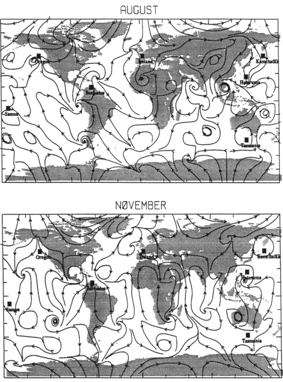
For use in the low resolution Golombek and Prinn (1986) model the emissions discussed in Chapter 3 are integrated onto the larger grid (Figure 4.1a). For the purposes of our study we define five geographical source regions (figure 4.1b). When estimating emissions from these five regions the distribution of emissions within each region is maintained as shown in Figure 4.1a. In Figure 4.1b the locations of the nearest model grid point to each of the five ALE/GAGE observation sites are marked by X's. The five stations are Macehead, Ireland (51N,10W), Cape Meares, Oregon (45N,124W), Ragged Point, Barbados (13N,59W), Point Matatula, American Samoa (14S, 171W), and Cape Grim, Tasmania (41S, 145E).

4.3 The Results:

We first ran the model forward for several years using the emissions for CFC13 derived from industry data (Figure 4.1 la). The output from this run at the five

100%

80%

60%

40%

20%

Figure 4.1: a) The pattern of the percent of global emissions from each grid point within the source regions based on an integration of the emissions shown

in Figure 3.1 b) the five source regions(shaded) and ALE/GAGE observation sites(X)

(b)

North America

Euox

Xi~ ii!iliili!

All 3 Southern Hemisphere

ALE/GAGE observation sites is defined as our "pseudo-data" and used to define the Xobs vector in equation (2.7).

The problem is then approached as if the magnitudes of the sources in the five regions in Figure 4. l b are not known. To begin the inverse runs the emissions from the five regions are initially set equal (which is deliberately a very poor guess) and the global total emission is initially set to be the same as used for the "pseudo-data". However, we do not subsequently constrain the global total emission during the inversion. The a priori emission error (in matrix C) is set equal to the emission strengths themselves thus giving a factor of two a priori uncertainty. Although this is overly pessimistic for CFCl3, it is

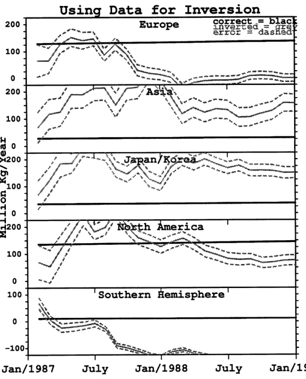
appropriate for the more biogenic trace gases such as methane and nitrous oxide. The inversion is then done once a month (of model integrated time) using the monthly averages of both Xobs and Xmodel. After each inversion the emissions E are updated as well as the estimated error (in C). Figure 4.2 shows the progression of the predicted source strengths and their uncertainties through a two year integration. As can be seen the derived source strengths converge rather rapidly to the true emissions used to generate Xobs despite the poor first guesses used for these emissions. The dashed lines corresponding to the error in the estimated emissions also converge as the inversion proceeds with convergence being greatest for Europe and the Southern Hemisphere. For example, the European source which started out at 65 ± 65 ends up 133 ± 20.

It is of interest to note that the North American region converges least rapidly toward the true solution. This may seem surprising considering there is an observing site (Oregon) on the west coast of this source region. Europe in contrast converges quickly despite the fact that it also has an observing site on its western margin (Ireland). The differences are due to a combination of station location and circulation. Both observing sites are climatologically upwind of these source regions but the Oregon station is a significant distance from the maximum North American source grid points (see Figure 4.1) whereas the Ireland station in this model is located at one of the maximum European source grid points. Figure 4.3 shows the 667 mb monthly mean streamlines in the 3-D model for February, May, August, and November. The locations of the nearest grid points to the ALE/GAGE stations are shown as black squares in this Figure. The winds consistently lack a strong easterly component at the Oregon observation site. However, at the Ireland station there are times (e.g. August) when the flow has an easterly component thereby carrying European air over this station. The effect of this circulation is in fact more dramatic for the true location of the Ireland station. To illustrate this further, Figure 4.4 shows the time series of aX).IEk for Ireland and Oregon for a changing North American source. The evidence of the change in the North American source is

Using Pseudo-Data for Inversion

200

Europe

correct

error' das

100

Asia

GII

200

North

"erica

200

'Southern Aemisphere'

0-Jan/1987

July

Jan/1988

July

Jan/1989

Figure 4.2: Time progression of the estimated source strengths at each source during an inversion run. The dark solid line represents the industry based

emissions used to generate the "pseudo-data". The solid grey line is the estimated source strengths from the inversion process initalized with all

the sources equal. The dashed grey lines are the estimated range of error in the estimated emissions

FEBRUARY

MAY

Figure 4.3: Streamlines for 667 mb from the Golombek and Prinn(1986) low-resolution spectral model for (a) February and (b) May. The black squares are the grid point locations nearest to the five ALE/GAGE observing stations and the two possible new

RUGUST

•f

NOVEMBER

-- -- --- -- -- -

-Figure 4.3 continued: Streamlines for 667 mb from the Golombek and Prinn(1986) low-resolution spectral model for (c) August and (d) November. The black squares are the

grid point locations nearest to the five ALE/GAGE observing stations and the two possible new stations (refer to text).

Figure 4.4: Time series of the partial derivatives for two ALE/GAGE stations in the northern hemisphere related to the North American emissions (a) Ireland and (b) Oregon

Calculated monthly average P values (Grey), piece wise fit (Black)

Pseudo-Data run Residuals at Observation Sites

Figure 4.5: Time progression of the residuals corresponding to the estimated emission time series in Figure 4.2. Also shown (vertical axis on the right) is the corresponding partial derivative relating the model calculated

value to the source(s) shown in the right hand corner of each frame.

first seen at Ireland. In this model the Oregon station does not see air from the major Eastern North American source until it has circled back around the hemisphere. This shows up in Figure 4.4 since the effect of the North American source on Oregon is nearly zero after the first month. In Figure 2.1 it was clear that the Ireland station does not have this time lag for the European source.

Besides North America, it is evident from Figure 4.2 that convergence for the Asian and Japanese/Korean source regions is somewhat slower than for the other regions. Of course, the fact that they do eventually converge onto the true values in the two years is very promising. Figure 4.5 illustrates some of the key variables in the inversion process. The lighter grey line is the residual between the pseudo-data and the calculated mixing ratio using the estimated emissions. These values are shown for each observation site. The dashed lines bracket the standard deviation of the pseudo-data. The darker lines are some of the partial derviatives (defined in the upper right hand corner). In considering the Japanese and Asian sources, Oregon is the largest affected in the model of the five observation sites. We show the partial derivatives for Oregon due to both Japan and Asia in Figure 4.5. Looking at this graph, it is evident that the influence from Japan is greater (the partial derviative from Japan is the darker line). Thus, although the convergence is slower for both Japan and Asia than the other sources, we would expect Japan to converge faster of the two, and this is what we see. Furthermore, in Figure 4.1 it is apparent that the sensitivity of the ALE/GAGE network is expected to be less for these regions since there is not an observation site near them. Since the Asian and Japanese/Korean regions have substantial emissions of many trace gases (e.g. CH4 from

rice agriculture) it is therefore of considerable interest to ask where a station should be located to resolve sources in these regions.

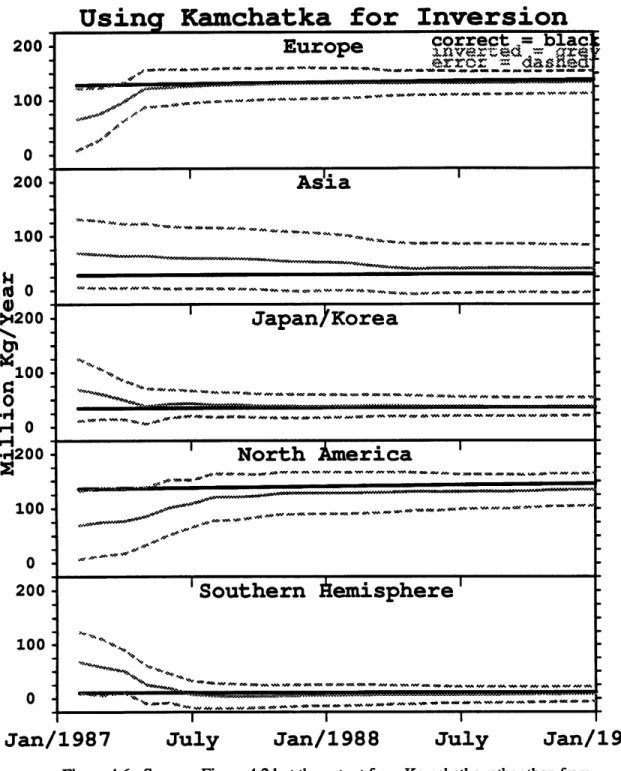
For this purpose we chose first to move the Oregon station (which is in fact no longer in operation) to Kamchatka (51N,156E) which is a peninsula off Russia just Northeast of Japan. The nearest grid point to this location is shown in Figure 4.3. We ran the same inversion procedure as above, only this time rather than using the grid point closest to the Oregon station we used the output from the grid point closest to Kamchatka to define Xobs using the true sources, to determine aX/DEk values, and to define Xmodel during the inverse procedure. The results from this inversion are shown in Figure 4.6. Comparing these results with Figure 4.2 it is apparent that the predicted Japanese source strength now converges much faster to the true value. This is expected due to the proximity of Kamchatka to Japan. Furthermore, Figure 4.3 illustrates that there is occasionally direct flow from Japan to the Kamchatka grid point. This is especially evident in February. However, the predicted Asian source strength converges even

Using Kamchatka for Inversion

200 Europe correct = blac

200 ',.''-vt" nver-ed -= ,r errot - dasd 100. . . . . . 0 200

Asia

Japan/Korea

o

A200

North merica

100 0 200

'Southern Aemisphere

Jan/1987

July

Jan/1988

July

Jan/1989

Figure 4.6: Same as Figure 4.2 but the output from Kamchatka rather than from Uregon is used as 'pseudo-data".

Using Hateruma for Inversion

200

Europe

uropenver ea = r 100 0 200-

Asia

200 -

Japan Korea

0

-

North America

200

Southern Aemisphere'

Jan/1987

July

Jan/1988

July

Jan/1989

Figure 4.7: Same as Figure 4.2 but the output from Hateruma rather than from

slower to the true value than when the station was located in Oregon. Looking at the streamlines in Figure 4.3, it is evident that there is not generally a transport of Asian air masses in this model to Kamchatka. So the air from Asia must travel around the hemisphere to reach Kamchatka, whereas it reaches the Oregon station after only travelling over the Pacific. Also note that the North American region now converges to the solution more rapidly than it did when using the Oregon location. This follows from the previous discussion of the North American source. Kamchatka is west of Oregon and therefore sees the effect of the Eastern North American source sooner than Oregon (but later than Ireland).

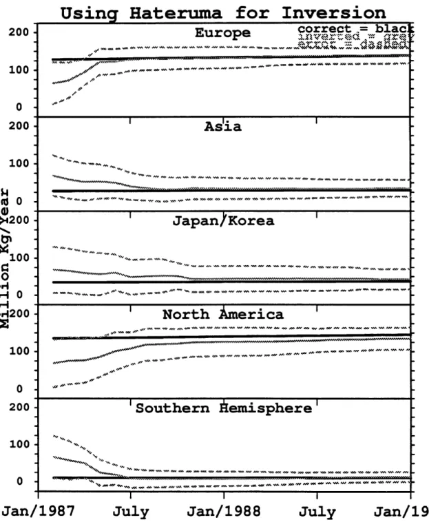
As seen above, Kamchatka helps resolve the Japanese/Korean source but it does not help with Asian sources. Recently the Japanese government has proposed opening a baseline station in Hateruma (24N, 123E) an island just east of Taiwan. To investigate this site we next replaced the Oregon station with Hateruma and repeated the inversion process to give the results shown in Figure 4.7. Now all of the sources converge rather well. Both Asia and Japan are resolved by the Hateruma location. This is also presumably a very promising location for deducing methane emissions since it is in some months located downwind from the most concentrated Asian region of rice paddies.

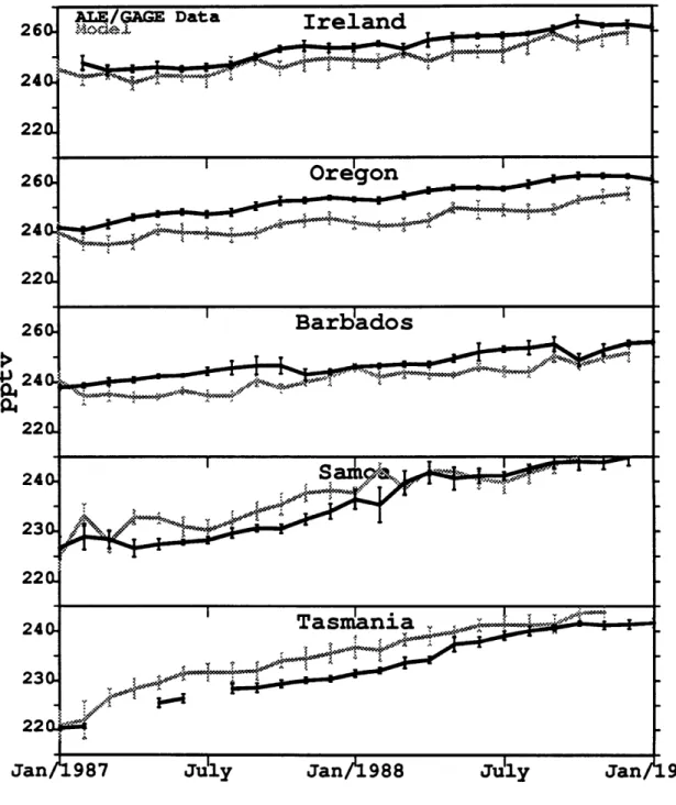
The above results show that a sparse (specifically ALE/GAGE) observational network can be used with the linear Kalman filter and a 3-D atmospheric chemistry-transport model to determine regional source strengths when the circulation is exact. However, when inverting using real observational data to determine sources the model circulation will no longer exactly match the real circulation that produced the observational data. An important question is how realistic does the model circulation need to be in order to obtain useful results? We address this question using our low resolution model with its imperfect circulation and the actual ALE/GAGE CFC13 observations. Figure 4.8 shows a time series of the model monthly averages obtained for CFC13 at the five ALE/GAGE stations using the emissions derived from industry data. Also shown are actual ALE/GAGE monthly average observations (with pollution episodes removed) at those locations and the standard deviations for both time series. There is a tendency for the model to underpredict concentrations in the northern hemisphere and overpredict them in the southern hemisphere due to a somewhat too rapid model interhemispheric circulation. Note that the model initiation process ensures that the model and observations both agree in January, 1987.

To address the effect of the differences in the above two time series on inversions, it is again assumed that the magnitudes of the emissions in the five source regions are unknown and as a first guess these magnitudes are set equal. Figure 4.9 shows the

220

2,4

Tas an

l.

,

240-23a

220.

Jan/1987 July Jan/1988 July

Figure 4.7: Monthly average concentrations and standard deviations from the model run(grey) with the industry based emissions and the

the ALE/GAGE data(black) with pollution removed for CFCl3.

Units are in parts per trillion by number (ppt).

Inversion

Jan/1987

July

Jan/1988

July

Jan/198 9

Figure 4.9: Same as Figure 4.2 only now the real ALE/GAGE data was used as the observations in the inversion process.