Computational regulatory genomics : motifs, networks, and dynamics

(1)

Computational Regulatory Genomics:

Motifs, Networks, and Dynamics

by

Pouya Kheradpour

B.S. Computer Science, University of Illinois at Urbana-Champaign (2005) M.S. Computer Science, University of Illinois at Urbana-Champaign (2005)

Submitted to the Department of Electrical Engineering and Computer Science in partial fulfillment of the requirements for the degree of

Doctor of Philosophy in Computer Science

at the

MASSACHUSETTS INSTITUTE OF TECHNOLOGY

February 2012

c

Pouya Kheradpour, MMXII. All rights reserved.

The author hereby grants to MIT permission to reproduce and

distribute publicly paper and electronic copies of this thesis

document in whole or in part.

Author . . . .

Department of Electrical Engineering and Computer Science

February 3, 2012

Certified by . . . .

Manolis Kellis

Associate Professor of Computer Science

Thesis Supervisor

Accepted by . . . .

Leslie A. Kolodziejski

Chair of the Committee on Graduate Students

(2)

(3)

Computational Regulatory Genomics: Motifs, Networks, and

Dynamics

by

Pouya Kheradpour

Submitted to the Department of Electrical Engineering and Computer Science on February 3, 2012, in partial fulfillment of the

requirements for the degree of Doctor of Philosophy in Computer Science

Abstract

Gene regulation, the process responsible for taking a static genome and producing the diversity and complexity of life, is largely mediated through the sequence specific binding of regulators. The short, degenerate nature of the recognized elements and the unknown rules through which they interact makes deciphering gene regulation a significant challenge.

In this thesis, we utilize comparative genomics and other approaches to exploit large-scale experimental datasets and better understand the sequence elements and regulators responsible for regulatory programs. In particular, we develop new computational approaches to (1) predict the binding sites of regulators using the genomes of many, closely related species; (2) understand the sequence motifs associated with transcription factors; (3) discover and characterize microRNAs, an important class of regulators; (4) use static predictions for binding sites in conjunction with chromatin modifications to better understand the dynamics of regulation; and (5) systematically validate the predicted motif instances using a massively parallel reporter assay.

We find that the predictions made by our algorithms are of high quality and are comparable to those made by leading experimental approaches. Moreover, we find that experimental and computational approaches are often complemen-tary. Regions experimentally identified to be bound by a factor can be species and cell line specific, but they lack the resolution and unbiased nature of our predictions. Experimentally identified miRNAs have unmistakable signs of being processed, but cannot provide the same insights our machine learning framework does. Further emphasizing the importance of integration, combining chromatin mark annotations and gene expression from multiple cell types with our static motif instances allows for increasing our power and making additional biologi-cally relevant insights.

We successfully apply the algorithms in this thesis to 29 mammals and 12 flies and expect them to be applicable to other clades of eukaryotic species. Moreover,

(4)

we find that our performance has not yet plateaued and believe these methods will continue to be relevant as sequencing becomes increasingly commonplace and thousands of genomes become available.

Thesis Supervisor: Manolis Kellis

(5)

Acknowledgments

First and foremost, I am deeply indebted to my supervisor Manolis Kellis for his guidance throughout my doctoral work and his consistent encouragement as I explored various aspects of regulatory genomics. Much of this thesis would never had completed had it not been for his sustained enthusiasm and direction. I would also like to thank David Gifford and Martha Bulyk for graciously agree-ing to be my committee members and for their advice toward completagree-ing my dissertation and regarding my future career.

Science frequently benefits from collaboration and this work is no exception; many members of the Kellis Lab have undeniably influenced this thesis, partic-ularly Alexander Stark, Leopold Parts, and Jason Ernst. Further, many of the results presented within this thesis were possible only because of data and ex-perimental work from the labs of Bradley Bernstein, Tarjei Mikkelsen, Kerstin Lindblad-Toh and the ENCODE, modENCODE, 12 fly, and 29 mammal consortia. During the past six and a half years I have had numerous comments and sug-gestions during my presentations and as part of these consortia, much of which positively influenced this thesis and for that I am grateful.

People require social interaction in order to maintain happiness and sanity, a fact that has been particularly true for me during my longest and most un-structured stage of development: graduate school. For providing me with this necessity, I would like to thank Seb Neumayer, Matt Rasmussen, Chris Evans, John Kelleher, Mike Lin, and especially Tracy Tat.

I have been truly fortunate to have two aunts, Khalehs Simin and Monir, and their families in the Boston area. They have opened their homes to me and kept me well nourished on countless occasions. Finally, I have to thank my parents, Albert and Jacklin, and my siblings Saba and Nima, for their unconditional love and continued support in pursing my interests.

(6)

(7)

Chapter 1 Introduction

1.1 Motivations

While gene regulation is vital to all life, our understanding of the underlying players and their precise roles remains incomplete. This thesis presents the de-sign and application of algorithms seeking to increase our knowledge of this basic process. Interest in computational regulatory genomics has greatly increased in recent years due to rapid advances experimental techniques, particularly the ex-ponential drop in the cost of sequencing.

The rapid rate of this advancement is apparent when examining publications

in the field. In 2000, the first draft of the Drosophila genome was published (∼120

megabases; Adams et al., 2000). A year later a decade long project culminated

with the publication of the first draft of the human genome (∼3 gigabases; Lander

et al., 2001; Venter et al., 2001). Today we have the sequence of 12 flies (Stark et al., 2007b; Drosophila 12 Genomes Consortium, 2007), dozens of mammals (Lindblad-Toh et al., 2011), and hundreds of additional eukaryotes (Kersey et al., 2009). Further, sequencing is now applied to even individuals of a species with dozens already sequenced and hundreds planned (Kaiser, 2008).

We benefit from this new abundance of data throughout this thesis — from predicting regulators, the patterns they recognize, to their specific instances in the genome. We also use these technologies to predict regulators and test them

(12)

using a high throughput enhancer assay. This dramatic rate of technological ad-vancement has made it difficult to predict the potential scope and direction of research making it an exciting time to be involved in computational biology.

1.2 Relevant biology background

This section will provide an overview of the biological concepts necessary to un-derstand the work in this thesis. The interested reader is encouraged to consult a more thorough treatment of the relevant topics, which is available in text books on molecular biology (Alberts et al., 2002; Watson et al., 2007; Lodish et al., 2007), gene regulation (Latchman, 2010), and computational biology (Durbin et al., 1998; Jones and Pevzner, 2004) and through online resources (e.g., Wikipedia). This treatment will also ignore most exceptions (which exist for nearly every biologi-cal statement) unless they are necessary for understanding a concept in this thesis.

1.2.1 Basics of molecular biology

All life on earth is made up of building blocks called cells. Genetic material in the form of deoxyribonucleic acid (DNA) is found in nearly all of these cells and encodes the primary “blueprints” for the development and response of the cells to external stimuli. This thesis will focus on eukaryotes, a class of organisms which includes fungi, plants and animals and for which most of the DNA is found in the nucleus. The language of DNA has a 4 character system of adenine (A), cytosine (C), guanine (G) and thymine (T), which are referred to as bases (bp) or nucleotides (nt). DNA is structured as a double-helix with complementary base-pairing (A to T, G to C) to facilitate easy replication, a feature noted since its initial characterization (Watson and Crick, 1953).

DNA is organized into chromosomes which are essentially long strings of the 4 bases. Obtaining these strings is the desired result of sequencing, but sequenc-ing errors and repetitive regions can complicate the complete recovery of each

(13)

mRNA

Func�on

Protein

DNA

transla�on

microRNAs

various modiﬁca�ons

Regulated by:

folding

transcrip�on factors

transcrip�on

Figure 1-1: Central dogma of molecular biology and an incomplete list of the major regulators involved.

chromosome’s sequence. Chromosomes contain specific substrings that encode functional elements. These functions can overlap with the same base having mul-tiple roles. Finding the coordinates of specific classes of functional elements will be one of the primary focuses of this thesis.

Large areas of the genome (from tens to as many as millions of bases) are transcribed into ribonucleic acid (RNA) by RNA polymerase proteins and are re-ferred to as genes. The direction of RNA synthesis (like DNA synthesis) is always

the same: from 50 to 30 (these refer to specific atoms in the chemical backbone of

DNA and RNA) and starts from the transcription start site (TSS) and continues until the transcription end site (TES; also known as the poly(A) site). DNA/RNA sequences in this paper will always be indicated in this order. Compared to DNA, RNA has specific chemical differences, including the nucleotide uracil (U) instead of T and does not always exist in a double-stranded form. RNAs take on a num-ber of roles in the cell and for some viruses can even be the primary carrier of genetic information.

Messenger RNAs (mRNAs) and are one of the primary types of RNAs en-coded by the genome. They are transcribed (or expressed) and then are processed (‘spliced’) removing sections referred to as introns leaving the exons. These

(14)

ma-TF2

TF1

miRNA1

Figure 1-2: A simple model of gene regulation. Regulators (top) each have an associated motif to which they bind. Transcription factors (TFs) bind near the

TSSs of genes they regulate, while microRNAs (miRNAs) bind to the 30 UTRs of

mRNAs.

ture transcripts are then translated into proteins using a code based on sliding non-overlapping windows of length 3. Each of the 64 3-base sequences (or codons) specifies one of 20 amino acids. Translation always begins with an AUG and ends with a UAA, UAG, or UGA. The portion of the processed mRNA that is

un-translated before the coding portion is referred to as the 50 UTR and the portion

following it is the 30 UTR. The transcription of DNA to RNA and the subsequent

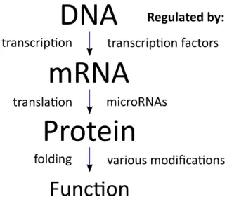
translation to proteins is referred to as the central dogma of molecular biology (Figure 1-1).

In eukaryotes chromosomes are wrapped around proteins called histones cre-ating nucleosomes. Both the DNA and histones can undergo semi-stably inher-ited covalent changes referred to as epigenetic modifications. Experimental tech-niques, such as ChIP-chip or ChIP-seq (Figure 1-4), are used to read the mod-ification state of each region of the genome (with resolution depending on the type of modification and the technique). Cataloging the modification state (or epigenome) is a substantial effort because many dozens of known modifications exist and must be annotated for each cell type (Bernstein et al., 2010; Celniker et al., 2009; Consortium, 2011b). These changes are correlated with various func-tional properties (Suzuki and Bird, 2008; Kouzarides, 2007; Ernst and Kellis, 2010), a fact that we will exploit in this thesis when predicting functional regions of the genome.

(15)

1.2.2 Gene regulation

While every cell in the body contains essentially the same DNA, cells themselves have dramatically different morphologies, behavior, and functions. This diversity is largely driven through the specific regulation of which genes are active in a cell. In turn, regulation occurs in every step between the DNA sequence and protein function (Figure 1-1). This section will briefly go through the mechanisms through which this occurs.

In vertebrates, some genes are responsive to DNA methylation near their up-stream of their TSS. DNA methylation can effectively turn off a gene (Suzuki and Bird, 2008) and can be stably inherited across cell devisions. In mammals most cytosines (C) that are followed by a guanine (G) are methylated. Because of the specific chemistry involved, methylated cytosines have a propensity to be mutated to thymine (T). Consequently the genome as a whole is depleted of CG dinucleotides. CpG islands are particularly common near housekeeping genes where DNA is not methylated in the germline and consequently CGs are not depleted.

Transcription itself is a five step process: pre-initiation, initiation, clearance, elongation and termination. The primarily regulators involved in this process are proteins called transcription factors (TFs). Each TF recognizes a specific pattern to which it binds. This sequence, called a motif, can be of variable length (5-20+ bases) and can be degenerate (e.g., recognizing either an A or a G at a specific position). Further, TFs can bind a variable distance from the gene: while there is a clear enrichment of TF binding sites near the genes they target, there are also examples of distal binding sites, called enhancers, many thousands of bases away from a TSS. The various steps of transcription can be individually regulated as well: for example, polymerase can pause at a promoter and fail to produce full length transcripts (Core and Lis, 2008).

The product of transcription is a precursor mRNA (pre-mRNA). The subse-quent splicing is regulated through the binding of factors called exonic/intronic

(16)

splicing enhancers/silencers (reviewed in Wang and Burge, 2008). Alternative splicing, along with alternative transcription start and end sites, can lead differ-ent isoforms of the same gene. Currdiffer-ent evidence suggests that more than two-thirds of human genes and two-fifths of Drosophila genes undergo some form of alternative splicing (Benjamin J., 2006), making it an important source of diver-sity for multicellular organisms. Although not explicitly discussed in this thesis, many of the approaches utilized here are also applicable to predict instances of splicing-related regulators.

After splicing the mature mRNA is exported from the nucleus into the cy-toplasm where it is ready for translation. Several regulators including pumilio proteins (Wharton et al., 1998) and microRNAs (miRNAs) can bind to the RNA through sequence specificity and influence degradation or translation of the tran-script.

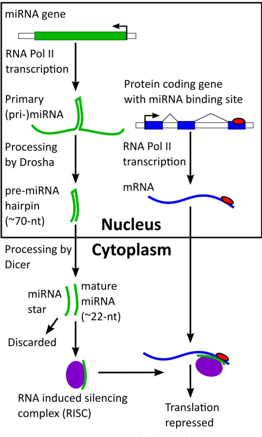
MicroRNAs are one of the most important regulators (reviewed in Winter et al., 2009; Bartel, 2004) and are of particular interest to this thesis. MicroRNA genes, which can be over 1 kb in length, are transcribed from the genome and

fold into ∼80-nt hairpin (Figure 1-3). These are then processed first in the

nu-cleus and then in the cytoplasm to create a short (∼22-nt) mature miRNA. These

short RNAs bind to the 30 UTR and sometimes coding region (Stark et al., 2007b;

Schnall-Levin et al., 2010) of a gene. Recognition of bases 2-7 of the miRNA (the seed) through canonical base pairing (A-U, G-C, not G-U) is largely responsible for the specificity of a miRNA in animals. Additional strength is added by a match to the 8th base, and having a match that is followed by an A and base pairing to the remaining portion of the miRNA (Lewis et al., 2005). Recognition by a miRNA leads to repression of the target mRNA effectively reducing the expression of a gene.

(17)

Protein coding gene

with miRNA binding site

mRNA

RNA Pol II

transcrip�on

Processing by

Dicer

Processing

by Drosha

RNA Pol II

transcrip�on

pre‐miRNA

hairpin

(~70‐nt)

Primary

(pri‐)miRNA

miRNA gene

Cytoplasm

Nucleus

Discarded

miRNA

star

RNA induced silencing

complex (RISC)

mature

miRNA

(~22‐nt)

Transla�on

repressed

Figure 1-3: Biogenesis and function of miRNAs.

(18)

1.3 Comparative genomics

Species on earth can be placed into a tree or phylogeny indicating their relation-ships (incomplete lineage sorting and horizontal gene transfer make this only roughly true, however we will ignore it in this thesis as it is relatively rare in the species we consider). When species have experienced sufficiently little diver-gence, genomes can be aligned to predict orthologous bases and identify specific mutations. A number of procedures exist for this problem and whole genome alignment is an active area of research. We use alignments provided by the UCSC genome browser which are generated using MULTIZ (Blanchette et al., 2004).

Comparative genomics is the technique of taking advantage of this evolution-ary history to better understand the genome. It can be difficult to predict even well specified genomic elements such as protein coding genes because we do not know all the rules that govern them. A popular and long successful strategy is essentially identify places that have a conspicuous reduction of mutations (Rubin et al., 2000; Kellis et al., 2003). Of course the cell cannot see the evolutionary his-tory of a segment of DNA. However, a lack of mutations suggests that a segment is important and thus undergoing purifying selection. Beyond a lack of muta-tions, for some elements such as genes the specific pattern of mutations that do occur can be suggestive of this specific function (evaluated in Lin et al., 2008).

This thesis will make extensive use of comparative genomics to predict func-tional elements. As we will show, we have sufficient power now to discover regulatory motifs with the number of species available. However, in most cases we still do not have sufficient signal to find short, poorly specified motif instances with high specificity. As more genomes are sequenced, the specific mutational pattern can be examined to determine the likelihood of a position evolving like a motif match. Consequently, comparative algorithms will continue to be of interest and will have to be designed to deal with additional genomes.

(19)

1.4 Relevant experimental techniques

This section will give an overview the large-scale experimental techniques utilized in this thesis (with the exception of MPRA, which will be described in Chapter 6). Understanding these techniques and their potential drawbacks is important for interpreting the results of this thesis and understanding the conclusions drawn.

1.4.1 DNA Sequencing

DNA sequencing refers to the process of obtaining the order of bases in a DNA molecule — data that is absolutely necessary for essentially all the analysis found in this thesis. Substantial efforts over the past few decades have led to a dra-matic reduction in the cost of sequencing (Schuster, 2008), which has had marked changes to how many molecular biology experiments are carried out.

Sanger sequencing, originally described in the mid-1970s (Sanger et al., 1977), was one of the first sequencing techniques and also the primary method used to sequence all the genomes utilized in this thesis. The basic protocol involves using labeled dideoxynucleotide triphosphates as DNA chain terminators. By running on a gel the product of the reaction of a sample with each of the four dideoxynucleotides (and the deoxynucleotides), one can read the bases in order by comparing the relative sizes of the resulting synthesized DNA. While the ini-tial technique was a labor intensive process, alterations to the original chemistry and automation procedures led to the feasibility of sequencing large mammalian genomes (reviewed in Alterovitz et al., 2009).

Because this technology was only able to produce contiguous sequences of length no greater than a few hundred bases, additional techniques were neces-sary for decoding larger genomic regions (e.g., entire chromosomes). The whole-genome shotgun approach is presently the dominant strategy for this purpose and was first applied to an animal genome to sequence Drosophila melanogaster (Adams et al., 2000). This approach fragments the genome into smaller pieces which are selected at random for sequencing. Subsequent computational

(20)

tech-niques are then used to assemble these fragments by utilizing their overlapping base pairs (Batzoglou et al., 2002; Huang et al., 2003). Because of this random selection procedure, regions of the genome can be missed by chance requiring a high coverage of sequencing in order to ensure each base is likely to be sequenced at least once.

Significant pressure to further reduce the price of sequencing led to the de-velopment of sequencing techniques that were highly parallelized and able to decode many more bases at a given cost (Shendure and Ji, 2008). Two commercial sequencing platforms based on a cyclic-array procedure (Shendure et al., 2005; Margulies et al., 2005) that produced data used in this thesis include 454 Genome Sequencers (Roche Applied Science) and the Illumina Genome Analyzer. These produce shorter contiguous segments, but with a vastly higher total amount of sequence. This made these technologies particularly suitable for sequencing miR-NAs (used in Chapter 4) and for ChIP-seq (used in Chapters 2, 3, 5), although genome assembly using these short reads has also been investigated (Zerbino and Birney, 2008).

Sequencing and the subsequent assembly can suffer from a number of prob-lems that can lead to missing or inaccurate sequence (Pop et al., 2002). The algo-rithms presented in this thesis, particularly that of Chapter 2, are designed to be robust against these errors by only minimally penalizing them. Moreover, many of the results presented in this thesis are statistical in nature and consequently are not strongly effected by the relatively few errors that occur due to sequencing.

1.4.2 mRNA expression analysis

While all cells have essentially the same DNA, a different complement of genes is expressed in each cell type. Consequently, determining the specific genes that are active in a given sample of cells is of great interest to understanding the under-lying biology. While it is generally desired to identify the specific proteins that are active in a cell type, this is technically difficult (Garbis et al., 2005).

(21)

How-ever, assaying nucleic acids is considerably simpler and very frequently used as a surrogate for the protein levels.

One popular approach for measuring the level of mRNAs in a sample is the DNA microarray (Schena et al., 1995). Microarrays contain tens to millions spots each with many copies of a single stranded DNA probe. Because the location of these probes is known, by placing a sample of nucleic acid (usually DNA com-plementary to an mRNA sample) and identifying the level to which the spots hybridize to the sample, a quantitative measure of the amount of RNA can be ob-tained. DNA microarrays can be made either using cDNA probes corresponding to fragments of mRNAs (Cheung et al., 1999; Duggan et al., 1999; DeRisi et al., 1996) or using synthesized oligonucleotide arrays (Irizarry et al., 2003).

cDNA microarrays are generated from a library of mRNAs and have probes that can be hundreds of base pairs long. However, because it is difficult to deposit consistent amounts of probe in each spot, generally two samples are hybridized to each array, using a separate florescent label for each. By comparing the rela-tive ratio of the two colors for each spot, an estimate of the abundance of each transcript across multiple samples can be made.

In contrast, oligonucleotide arrays have probes that are arbitrarily synthesized sequences of relatively short length (10-200 bp). Because these sequences may not uniquely identify a transcript and in order to reduce noise, typically many such probes are designed for each mRNA and the expression level of each transcript is estimated by combining these values (Irizarry et al., 2003). In Chapter 6, we exploit this synthesis procedure not for expression analysis but rather to produce a large library of arbitrary sequences.

Both DNA microarray technologies suffer from what can be very high noise levels (Reis-Filho et al., 2006). Moreover, due to the design assumptions, microar-ray manufacturers advise against the comparison of expression between genes and cross-hybridization between similar sequences can make it difficult to inter-pret results. Consequently, as sequencing has become cheaper RNA-seq tech-nologies (Mortazavi et al., 2008; Wang et al., 2009) are starting to replace DNA

(22)

microarrays.

1.4.3 Chromatin immunoprecipitation

Beyond the static genome lies a dynamic collection of proteins and modifications that decorate the genome. As described above, in this thesis we will want to know where TFs bind to the genome and what chromatin modifications exist in each genomic region. Chromatin immunoprecipitation (ChIP; Solomon et al., 1988) followed by the application to a microarray (ChIP-chip; Ren et al., 2000; Iyer et al., 2001) or sequencing (ChIP-seq; Robertson et al., 2007) permit the assaying of these genomic features in a dynamic manner (Figure 1-4). The same type of arrays can be used for ChIP-chip as are used for expression analysis. However, because there are many more genomic features that are candidates for protein binding compared to the number of mRNAs, producing arrays for ChIP-chip can be a much more challenging problem and require trade-offs in terms of coverage and cost.

A number of potential issues exist with both ChIP-chip and ChIP-seq. First, they inherit the problems with their underlying technology and can have a sig-nificant error rate (Buck and Lieb, 2004). For ChIP-seq, repetitive regions and sequencing errors make mapping the reads to the genome can be a significant challenge (Park, 2009).

Beyond technical issues, ChIP techniques, when applied to TFs, are inherently only able to find regions bound in the specific sample and are unable to find other potential binding sites for a factor. Further, the high rate of turnover be-tween species (Odom et al., 2007) suggests that many binding sites may not be selectively functional making the results of ChIP experiments difficult to put in context. Finally, they are unable to distinguish between sequence specific binding and non-specific binding due to highly accessible regions, which may constitute a large number of the bound regions (Li et al., 2008).

(23)

Use whole‐cell

extract

to measure

background

Reverse crosslinks

and purify DNA

Use an�body to select

only DNA with desired

proteins bound

Isolate and fragment

DNA with proteins

a�ached

Cells with proteins

cross‐linked to DNA

Sequence and

match to genome

ChIP‐seq

Apply to �ling

microarray

ChIP‐chip

ACGTAATACGATACAGAGATACA GTTGGACATGGACACG GTCCCAACAGGTACACAGTAC GTACATTAAT TTAACACACAGAA CCCAAATTATAGGGAA

Figure 1-4: Diagram of chromatin immunoprecipitation (ChIP) followed by as-sessment with microarray (chip) or sequencing (seq).

(24)

1.5 Common data used

1.5.1 Comprehensive collection of known motifs

Known motifs were collected primarily from large scale datasets or databases, but with significant manual annotation. For human, we collected human, mouse, and rat motifs from Transfac (version 11.3; Matys et al., 2003), vertebrate motifs from Jaspar (version 2008; Sandelin et al., 2004), and large scale systematic motifs generated by Protein Binding Microarrays (Berger et al., 2006; Badis et al., 2009; Berger et al., 2008). For Drosophila we used fly motifs from Transfac and Jaspar in addition to motifs collected from various literature sources (Sen et al., 2010; Reed et al., 2008; Noyes et al., 2008a,b; MacArthur et al., 2009; Down et al., 2007; Ivan et al., 2008; Wasserman and Sandelin, 2004). Names for the motifs were standardized by factor name (in human some families were collapsed if their motifs were similar enough; fly motifs were named by their fly base symbol). Hierarchical clustering of mammalian motifs is performed using centroid linkage and a cutoff of 0.95. This cutoff is high enough where the motifs essentially match the same genomic locations and is used only for identifying redundancy. For each cluster only the motif closest to the centroid is retained.

1.5.2 Genome annotations

Because the work in this thesis is centered around model organisms, we are able to exploit available annotations. When performing motif instance prediction, it is important to exclude regions that may have other sources of evolutionary con-straint (e.g., coding sequence) and regions that are difficult to align (e.g., repeats).

Consequently, all simple repeats, repeat masked regions, coding regions, 30UTRs,

exons from non-coding genes, and chromosomes Y and M are excluded unless otherwise specified. Simple repeats and repeat masked regions are taken from UCSC for the appropriate assembly (Kent et al., 2002). Fly gene annotations for dm3 were taken from Flybase v5.28 (Tweedie et al., 2009) and miRBase v15

(25)

(Griffiths-Jones et al., 2008). Human hg18 annotations (used in Chapters 2 and 5) are taken from GENCODE v2b (Harrow et al., 2006); hg19 annotations (used in Chapter 3) are taken from Gencode v4.

1.6 Thesis overview

This thesis deals with using computational approaches to better understand gene regulation. The contributions include:

• A novel, practical algorithm for predicting comparative motif instances (Chapter 2). We analyze the performance of the algorithm in recovering motifs in the context of experimental and functional datasets and for differ-ing numbers of species. We conclude that additional species will allow us to predict additional instances at the same confidence. To make this analysis possible, we develop a number of high-performance computational tools. • The systematic annotation of motifs for hundreds of human ChIP-seq

datasets (Chapter 3), appropriate for use with the method developed in

Chapter 2. We use statistical corrections for enrichment and carefully

chosen controls to correct for various issues and are able to find: (1) the most accurate motif for a TF; (2) a handful of unvalidated, novel motifs; (3) cooperating and antagonizing factors; and (4) meaningful differences in binding of the same factor between cell types. We do a thorough anal-ysis of the results and find many factor relationships that are confirmed in the literature and make several additional predictions appropriate for follow-up.

• Methods for computationally predicting microRNA (miRNA) hairpins and

their corresponding 50 cleavage sites using comparative and structural

in-formation (Chapter 4). To predict these regulators we use a customized random forest algorithm and achieve over 4,500-fold enrichment for real hairpins over random hairpins in the genome. We find that our

(26)

perfor-mance is better than a competing algorithm that was run on the same data. Predicting the mature miRNA produces additional motifs for use with our motif instance algorithm; we use an SVM and update several previously made predictions, leading to a significant update in the target spectra. • The annotation of cell line specific factors in human and fly using chromatin

modifications (Chapter 5). We find: (1) our comparative motif instances can be reliably used to predict key regulators of cell types; (2) these regulators can be classified as activators or repressors by how their enrichment signa-tures correlated with the expression of the regulators in the same cell types; and (3) the enrichments of activator motifs and their correlation with expres-sion can be used to classify chromatin marks or states in terms of activator potential.

• The systematic testing of the predictions made in Chapters 2 and 5 (Chapter 6). We apply a massively parallel reporter assay (MPRA) to measure the en-hancer activity of thousands of sequences centered on motif instances and their engineered manipulations. In doing so, we significantly increase the number of experimentally validated enhancers and careful statistical analy-sis leads to a number of insights: (1) 145-bp is often sufficient to capture the enhancer activity when centered on motif instances; (2) enhancers centered

on comparative motif instances are ∼2 times more likely to be functional

as those centered on random motif matches; (3) several other properties are correlated with sequences that have strong enhancer activity, including chro-matin mark dip scores (an indication of nucleosome exclusion), motif match strength, and the enrichment of motifs for other factors; (4) manipulating the motif match affects expression consistent with the specificity indicated by the PWM: disruptive mutations that would prevent TF binding eliminate enhancer activity, whereas mutations permitted by the PWM do not affect enhancer activity; (5) disrupting the binding sites for repressors can lead to an increase in expression in the cell type where the repressor in active; and

(27)

(6) together these results validate our motif instances and our factor/cell-line predictions.

(28)

(29)

Chapter 2 Regulatory motif instance prediction

This chapter will describe and evaluate an algorithm for predicting functional motif instances using multiple, closely related species. We define functional motif instances as those that would result in a reduction of fitness of an organism if disrupted, although we also expect them to be more likely to be biochemically active than a simple motif match. The comparative motif instances produced here will be used in Chapter 5 to examine the relationship between motif instances and chromatin modifications and then systematically experimentally validated in Chapter 6. While I was responsible for almost all aspects of the implementation and analysis, some of this work, particularly the initial algorithmic design and the Drosophila results, were done as part of a collaboration with Alexander Stark. This chapter is based on results previously published in Kheradpour et al. (2007), Stark et al. (2007b), and Lindblad-Toh et al. (2011) with notable additions.

2.1 Introduction

Once the motif for a regulator has been determined, a natural desire is to pre-dict its functional locations. However, a consequence of short nature of most metazoan motifs (5-15 bp) is that they will frequently match the genome just by chance — a fully specified 6-mer will match a uniformly random genome once

(30)

Mouse Rat Dog Human

b

c

a

Figure 2-1: Challenges associated with motif instance identification using many aligned genomes (hypothetical motif matches are indicated in red). (a) The sim-ple, straightforward case is when an instance is found fully conserved in the orthologous position near a given gene. (b) Motif turn-around or alignment er-rors can lead to a motif match being found in a location proximal to one in the target genome, but not directly aligned. (c) Motif matches can be missing due to turn-over or sequencing errors. The motif instances can also be found far from a gene, making them difficult to assign.

of thousands of matches for such a motif, far more than the number of regions bound in an experimental assay (tens of thousands at most). The source of this discrepancy is not completely clear, but chromatin structure, lack of necessary co-factors or motif multiplicity, and incorrect models of binding have been proposed as possible explanations (Wasserman and Sandelin, 2004; Badis et al., 2009).

Consequently, the general approach toward motif instance prediction has been to increase power by looking for motif matches that are more likely to be associ-ated with functionality but less likely to occur just by chance. A popular way to do this is by finding regions of the genome that are enriched for a set of transcrip-tion factors known to act in concert (Berman et al., 2002; Schroeder et al., 2004; Philippakis et al., 2006). This has been successful because it requires only one genome but can predict sequences that have a high probability of functionality. However, these approaches are inherently require a set of motifs known to act together and are unable to find motif matches that occur in isolation.

An alternative approach that is able to find isolated binding sites is phyloge-netic footprinting, which exploits the preferential conservation of motif instances. Early work in this area mainly focused predicting motif instances that were per-fectly conserved in orthologous regions between two or more species (Sharan et al., 2003; Ettwiller et al., 2005; Lewis et al., 2005) whereas Ho Sui et al. (2005)

(31)

matched motifs to areas with conservation above some threshold. Conversely, Blanchette and Tompa (2002) used an alignment-free approach to find k-mers in orthologous promoters that were unusually well conserved and Moses et al. (2004) models binding using a strict phylogenetic model to find regions that evolve ac-cording to the motif and not the background. These methods were generally not designed to cope with large phylogenies of species containing sequencing and alignment errors.

In this chapter we present our own practical alignment-free phylogenetic foot-printing algorithm. We will then evaluate our method separately using 29 placen-tal mammals and 12 fruit flies. We expect this method to be generally applicable as long as whole genome alignments can be produced and there is sufficient total branch length.

2.2 Producing robust comparative motif instances

The complexity of large phylogenies leads to a number of issues that prevent sim-ple matching of motifs to conserved genomic regions. Sequence properties, such as dinucleotide biases, must be considered because they greatly influence the abundance of a motif and its observed mutation rate. Consequently, we produce control motifs specific to each motif we scan that are diverse and have similar properties to our original motif (Figure 2-2). Further, the low coverage genomes used for some studies (e.g., the 29 mammals) will lead to large gaps in the as-semblies for some species necessitating a scoring scheme that does not strongly penalize for a missing species in a dense species tree. Even with complete data, unannotated functional elements may match a motif and produce an apparently conserved instance, requiring the measuring of background level of conserva-tion. Because alignment algorithms are imperfect and motif turnover may lead to motifs appearing to have moved (Odom et al., 2007), we support shifts in the placement of motif instances in the alignment. These motif turn-over events represent conservation of function, not a phylogenetic relationship between the

(32)

4 Randomly select up to 10 motifs but only permit_{at most one motif per cluster} 1

Produce 100 shuffles of our original motif while roughly preserving the overall information content structure

Original motif

2 Filter motifs, requiring they match the genome

about as often (+/‐ 20%) as the original motif Genome sequence

3 Cluster the remaining potential control_{motifs at a correlation cutoff of 0.8}

Figure 2-2: Procedure for generating shuffled motifs.

corresponding bases. Consequently, our motif instances are produced using an alignment-free approach that has been used by others for similar purposes (Ward and Bussemaker, 2008).

For each motif in our database (see Section 1.5.1), 100 putative control motifs are generated by randomly shuffling the columns of each PFM (Figure 2-2). Be-cause the particular way the information content of a motif is ordered may affect the background level of conservation (e.g., a group of specified bases surrounded by unspecified bases may be more likely to be conserved by chance), we create three bins of information content and shuffle only within each bin. Each of the 100 shuffled motifs is then matched to the genome (as described in Section 2.3) and

only those that have ±20% the number of matches of the original motif are

(33)

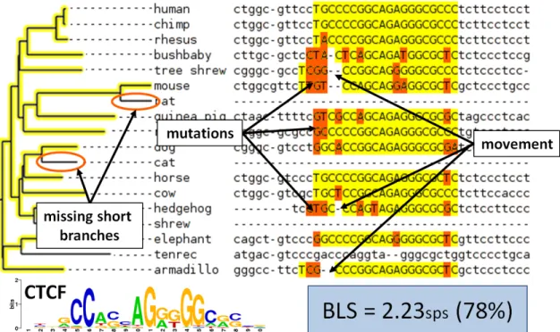
Figure 2-3: Example motif match to CTCF and corresponding computation of BLS. BLS is equal to the size of the smallest subtree that contains all the species with a motif match. The advantages of this approach over a simple measure of conservation are indicated. This example is illustrative and not all species used for 29 mammals study are included. BLS is measured here in substitutions per site (sps).

at a 0.8 correlation cutoff and up to 10 control motifs are chosen in random order, allowing only one motif per cluster. We find that the cutoff of 0.8 results in mo-tifs that are sufficiently dissimilar as to not frequently match the same sequences disrupting our statistics which assume independence.

Because we require identical base-composition and similar number of overall matches, for some motifs no control motifs can be generated and thus are not

amenable to our algorithm (this generally occurs for < 1% of motifs). The

algo-rithm does not permit lower quality controls and thus does not compromise the quality of motif instances.

Our analysis is centered around the same species as an input whole genome alignment, which is typically a model organism such as human, mouse, or Drosophila melanogaster. All the other species in the alignment are used as in-formants. For each motif match (Section 2.3) in the target genome, we compute

(34)

a branch length score (BLS; Figure 2-3)). This is done by using whole-genome alignments to identify the other species that have a motif match in the aligned position (expanding this to allow motif movement is described below). The BLS is then defined as the branch length of smallest subtree containing all species with a motif match.

We then produce a mapping between BLS and confidence (intended to ap-proximate 1 - false discovery rate; Figure 2-4) for each BLS (at 100 evenly spaced values from 0 to the total branch length of the tree) by computing the number of instances that reach that BLS score and comparing that to the number we would

expect to be according to the control motifs. Let ¯rb be the fraction of instances

for control motifs that have BLS score ≥ b, and let rb = nnb0 where nb indicates

the number of motif matches to our motif that have BLS ≥ b. We define the

confidence cb: cb = nb−¯rb×n0 nb = 1− ¯rb rb

notice that while cb will be negative if the control motifs are more conserved than

the original motif, because c0 = 0 and will always have the most instances, we

never report motif instances with less than 0 confidence.

This measure of alignment-free conservation does not use a fully specified model of evolution. However, because it empirically corrects for phenomena that would otherwise be difficult to model (e.g., conservation due to non-coding RNAs), we have found it to be useful in practice, which we will show in the remainder of this thesis.

Wilson score interval (Wilson, 1927) with z = 1 is applied to both r

(correct-ing downward) and rc (correcting upward) in order to produce a conservative

estimate of confidence in situations with few instances. This is essentially the same computation we use for evaluating enrichments (see Section 5.2). We also permit motif movement by repeating the procedure for each of the 32 windows

(35)

Matches to control mo�fs

Con

ﬁde

nc

e

N

umber

of

ma

tc

hes (i

n t

housa

nds)

Branch length score (BLS)

Matches to real mo�f

Conﬁdence 0.5 1.0 1.5 2.0 2.5 0.0 0 3 6 0.0 0.2 0.4 0.6 0.8 1.0 9

Figure 2-4: Computation of confidence score for motif instances of CTCF in mam-mals. The number of instances for the motif that reach each branch length is computed (dark blue). Control motifs are used to compute an expected back-ground level (light blue), correcting for alignment-free conservation by chance or due to overlap with unannotated elements. The fraction of the dark to light blue above results in the confidence score (red).

(36)

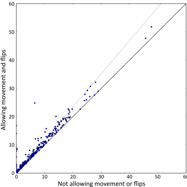
w =0, 5, 10, 20, . . . , 100, 120, . . . , 500 allowing both the motif and the control motifs to move w bases in the informant genomes relative to the position aligned to our target species. Consequently, for each confidence cutoff from 0.1, 0.2, . . . , 0.9 the BLS and w combination that results in the highest sensitivity is chosen. However,

permitting movement only modestly increases the number of instances (∼17% in

human) and consequently our method is still largely alignment driven (Figure 2-5).

In human, confidence prediction is done on only autosomes (non-X/Y/M chromosomes), and then instances are produced on the chromosome X using the mapping produced on the autosomes but with a tree produced on chromosome X. This is important to correct for the higher background level of conservation of chromosome X (Vicoso and Charlesworth, 2006). Chromosome Y is ignored because data in other species is incomplete (not all sequenced mammals were male) . Scaling and motif movement analysis shown below ignores instances on chromosome X (Figures 2-5, 2-10, 2-14 and 2-15).

2.3 Techniques for matching motifs

Typically, motifs are available as 4xN matrices indicating for each position the fre-quency of each base (position frefre-quency matrix; PFM). Before matching, PFMs are typically converted to PWMs by incorporating a background model and putting them into log space. In this thesis we use a pseudo count of 0.001 (to prevent undefined values) and a uniform background. In this chapter, we will generally

use a threshold corresponding to 4−8 as determined by TFM-Pvalue (Touzet and

Varre, 2007). Matching a single PWM to one genome is a straightforward com-putational task involving summing floats across each position and comparing to a cutoff. A number of tools are available for this task, including MAST (Bailey and Gribskov, 1998), storm (Schones et al., 2005), and AffinityProfile (Foat et al., 2006). For our purposes we needed a tool that could: (1) match motifs to multiple species, (2) scan in a window in the other species while avoiding the same match

(37)

0 10 20 30 40 50 60

Not allowing movement or ﬂips

All

o

wi

ng mo

veme

n

t

and

ﬂi

p

s

0 10 20 30 40 50 60

Figure 2-5: Number of motif instances (in thousands) for each human motif at 40% confidence when allow motif movement and flips or not. Solid line indicates no change whereas dotted line is a 17% increase (the overall proportion of additional instances).

(38)

being assigned to multiple matches in the target, while being (3) fast enough to feasibly match thousands of motifs to mammalian scale genomes. Here we de-scribe technical details of our motif matching software (written in C) that fulfills these requirements.

For each motif, all fully specified 8-mers that could begin a motif match are computed (recursively; motifs less than length 8 are padded with Ns). These are

put into a 48 entry lookup table so that while scanning the target species genome

a single lookup can produce a list of all potentially matching motifs. We found that this heuristic dramatically increases the speed of matching (about 10 times, for our typical mammalian runs).

Once we have found a motif match in the target species, we must determine which informant genomes also match. For this purpose, we compute the flanking matches to our motif in the target genome. These are used to eliminate the aligned regions in the informant species that are closer to some other motif match in the target species. This is an important step to avoid a single match in an informant species from making multiple target species matches appear conserved. Once the informant species with motif matches are determined, we compute the BLS using a parent tree representation of the phylogenetic tree.

Finally, many analyzes require computing enrichments by counting the num-ber of instances in each type of region. Because the resulting match files can be as large as 200 gigabytes compressed, most software to produce overlaps would fail when trying to load them into memory. To deal with this challenge we pro-duced software to determine overlapping regions for files sorted by chromosome then start position. Overlaps are then produced using the following algorithm (which is the same as the “chromsweep” algorithm independently implemented by BEDtools; Quinlan and Hall, 2010):

1 s t o r e d _ l i n e s = {}

2 w h i l e n e w _ l i n e = r e a d _ l i n e ( f i l e _ 1 ):

3 // when c o m p a r i n g p o s i t i o n s , also c o m p a r e c h r o m o s o m e s

(39)

5 // scan t h r o u g h list of s t o r e d e l e m e n t s and r e m o v e ones

6 // we will n e v e r o v e r l a p in a n o t h e r read in f i l e _ 1 line

7 for line in s t o r e d _ l i n e s in o r d e r : 8 if line . end < n e w _ l i n e . s t a r t : 9 d e l e t e s t o r e d _ l i n e s [ line ] 10 else if line . s t a r t >= n e w _ l i n e . s t a r t : 11 b r e a k // s h o r t c i r c u i t 12 13 // read in new l i n e s

14 w h i l e not ( eof ( f i l e _ 2 )) and

15 ( 16 i s e m p t y ( s t o r e d _ l i n e s ) or 17 s t o r e d _ l i n e s . last . s t a r t <= n e w _ l i n e . end 18 ): 19 line = r e a d _ l i n e ( f i l e _ 2 ) 20 if line . end >= n e w _ l i n e . s t a r t : 21 s t o r e d _ l i n e s . push ( line ) 22 23 // p r i n t out m a t c h i n g e l e m e n t s 24 for line in s t o r e d _ l i n e s in o r d e r : 25 if line . s t a r t <= n e w _ l i n e . end : 26 p r i n t new_line , line 27 else : 28 b r e a k // s h o r t c i r c u i t

The running time of this algorithm is O(f1+ f2+o) where f1 and f2 are the

number of lines in each file and o is the number of overlaps (we only examine a constant number of stored_lines more than we print or read in each iteration).

More importantly, memory usage is only O(omax) where omax is the maximum

number of elements a region in f1 overlaps in f2. Sorted motif matches are

au-tomatically produced by scanning chromosomes in alphanumeric sort order and sorted regions are produced by unix sort (which, depending on implementation,

(40)

Conf-idence No. motifs reaching confidence Total No. instances % examined bases covered No. TFs with a motif reaching confidence Total No. instances (best motif per TF) 0.0 630 55,021,406 80.6 335 35,366,716 0.1 540 15,817,545 45.3 294 11,181,918 0.2 492 8,385,913 26.0 270 6,068,955 0.3 435 4,697,272 14.3 252 3,495,271 0.4 375 2,675,802 7.7 225 2,050,302 0.5 293 1,449,752 3.9 188 1,175,237 0.6 216 707,141 1.7 151 595,984 0.7 129 269,944 0.6 101 240,849 0.8 56 90,464 0.2 45 80,138 0.9 16 33,822 0.1 14 29,080

Table 2-1: Basic statistics on the predicted human motif instances.

uses disk cache as necessary). Together these tools permit us to match hundreds of motifs to entire mammalian genomes with relative ease (on an appropriately sized cluster).

2.4 Validating the predicted mammalian regulatory

network

Of the 688 motifs initially in our database, 630 (representing 335 factors) were able to be matched at the required stringency and have at least one shuffle motif. The number of instances found at various cutoffs are indicated in Table 2-1.

ChIP-chip/seq is a popular experimental technique for determining the bind-ing sites of a factor in vivo (Section 1.4.3). However, because ChIP inherently does not capture binding events that occur in all cell types, and not all binding events are conserved, we do not expect perfect concordance between ChIP re-gions and comparative motif instances. Regardless, an enrichment in one relative to the other would suggest the validity of the motif instances because we expect functional motif instances to be more likely to be bound in vivo.

(41)

Factor Cell type Technology Num peaks Motif used Citation

CTCF CD4+ T_{ES (mouse)} Sequencing 21,544_{8,546 (+mouse)} Jaspar MA0139.1 Barski et al. (2007)_{Mouse: Goren et al. (2010)} ER MCF-7 Paired-end Tags 1,229 7 Transfac M00191 Lin et al. (2007a) Fos K562 CML Sequencing 18,963 7 Transfac M00926 Raha et al. (2010) FOXA2 Liver Promoter array 143

19 (+mouse) Jaspar MA0047.2 Odom et al. (2007) HNF1 Liver Promoter array 246_{23 (+mouse)} Jaspar MA0046.1 Odom et al. (2007) HNF4 Liver Promoter array 1,231_{99 (+mouse)} Transfac M01036 Odom et al. (2007) HNF6 Liver Promoter array 149_{20 (+mouse)} Transfac M00639 Odom et al. (2007) Myc K562_{ES (mouse)} Sequencing_{Promoter array (mouse)} 15,749_{2,399 (+mouse)} Transfac M00187 Raha et al. (2010)_{Mouse: Kim et al. (2008)} NF-κB GM12878 Sequencing 38,559 Jaspar MA0061.1 Kasowski et al. (2010) NRSF Jurkat T Sequencing 1,931 Transfac M00325 Johnson et al. (2007) p53 HCT116 Paired-end Tags 62,939 Transfac M00034 Wei et al. (2006) STAT1 HeLa-S3 Sequencing 41,530 Transfac M00224 Robertson et al. (2007) YY1 NT2/D1 Sequencing 11,018 Transfac M00651 Consortium (2011a)

Table 2-2: Listing of datasets and motifs used in human analysis. Datasets were identified from the literature and the peaks identified in the study were used after mapping to the appropriate assembly (if necessary) using liftOver (Kent et al., 2002). For factors that also had a dataset available in mouse, we show the number of peaks found in human that were bound in the orthologous mouse positions. When multiple motifs were available for a factor, we chose the one with the highest enrichment in the human dataset (ignoring conservation).

(42)

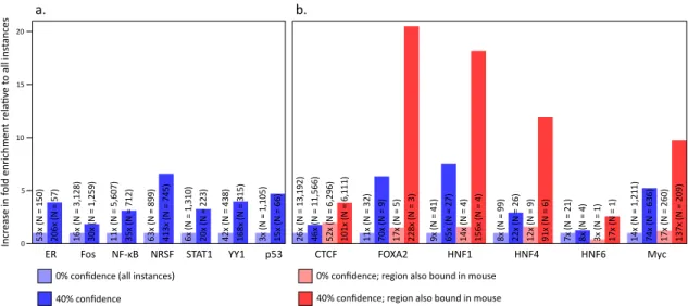
0% conﬁdence (all instances) 40% conﬁdence

0% conﬁdence; region also bound in mouse 40% conﬁdence; region also bound in mouse

Inc re ase in f ol d enr ic hme n t r el a� ve t o al l i ns ta nc es a.

ER Fos NF‐κB NRSF STAT1 YY1 p53

b. CTCF FOXA2 HNF1 HNF4 HNF6 Myc 0 5 10 15 20 5 3 x (N = 1 5 0 ) 2 0 6 x (N = 5 7 ) 1 6 x (N = 3 ,1 2 8 ) 3 0 x (N = 1 ,2 5 9 ) 1 1 x (N = 5 ,6 0 7 ) 3 5 x (N = 7 1 2 ) 6 3 x (N = 8 9 9 ) 4 1 3 x (N = 7 4 5 ) 6 x (N = 1 ,3 1 0 ) 2 0 x (N = 2 2 3 ) 4 2 x (N = 4 3 8 ) 1 6 8 x (N = 3 1 5 ) 3 x (N = 1 ,1 0 5 ) 1 5 x (N = 6 6 ) 2 6 x (N = 1 3 ,1 9 2 ) 4 6 x (N = 1 1 ,5 6 6 ) 5 2 x (N = 6 ,2 9 6 ) 1 0 1 x (N = 6 ,1 1 1 ) 1 1 x (N = 3 2 ) 7 0 x (N = 9 ) 1 7 x (N = 5 ) 2 2 8 x (N = 3 ) 9 x (N = 4 1 ) 6 5 x (N = 2 7 ) 1 4 x (N = 4 ) 1 5 6 x (N = 4 ) 8 x (N = 9 9 ) 2 2 x (N = 2 6 ) 1 2 x (N = 9 ) 9 1 x (N = 6 ) 7 x (N = 2 1 ) 8 x (N = 4 ) 3 x (N = 1 ) 1 7 x (N = 1 ) 1 4 x (N = 1 ,2 1 1 ) 7 4 x (N = 6 3 6 ) 1 7 x (N = 2 6 0 ) 1 3 7 x (N = 2 0 9 )

Figure 2-6: Enrichment of motifs in published experimental datasets. (a,b) Known motifs for each factor show an enrichment in experimental datasets which in-creases with alignment-free conservation. (b) Enrichment dramatically inin-creases for regions that are bound in both human and in the orthologous positions in mouse.

datasets (Table 2-2) and we do, indeed, observe increased enrichment of our

comparative motif instances (Figure 2-6). Enrichments are computed as the

ratio of the fraction of motif instances inside a region to the fraction of bases inside that region. For example, if 20% of a motif’s instances are bound by a given factor, but only 1% of the genome is bound, then we would report an enrichment of 20-fold. Moreover, this enrichment increases, often substantially, with increasing confidence (Figure 2-7) and is also seen for fly datasets (Figure 2-8), demonstrating the generality of this method.

In many cases, a larger proportion of the predicted motif instances do not overlap experimentally bound sites than is expected given the precision indicated by the confidence level. These may result from (1) an inaccurate confidence pre-diction, (2) false negatives in the experimental procedure, (3) the existence of a regulator with similar binding affinity, (4) regions bound in cell types not as-sayed, or a combination therein. It is, therefore, interesting to note that for CTCF, which has fairly consistent binding across cell types (Kim et al., 2007; Cuddapah et al., 2009) and whose binding specificity is not similar to that of any other factor

(43)

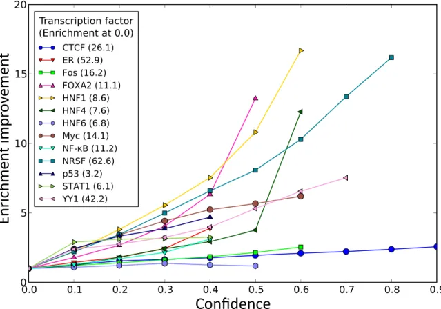
0.0 0.1 0.2 0.3 0.4 0.5 0.6 0.7 0.8 0 5 10 15 20 0.9 Transcription factor (Enrichment at 0.0) CTCF (26.1) ER (52.9) Fos (16.2) FOXA2 (11.1) HNF1 (8.6) HNF4 (7.6) HNF6 (6.8) Myc (14.1) NF-κB (11.2) NRSF (62.6) p53 (3.2) STAT1 (6.1) YY1 (42.2)

Conﬁdence

Enr

ic

hmen

t i

mpr

o

ve

men

t

Figure 2-7: Enrichment of corresponding motifs in bound regions. Most factors show consistent and substantial increases in enrichment with increasing confi-dence. Motif enrichments divided by enrichment at 0.0 confidence (i.e. all motif instances).

(44)

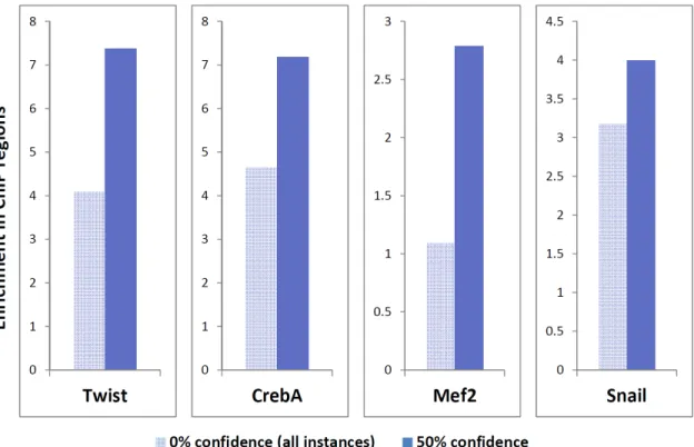
Figure 2-8: Increase in enrichment is also seen for fly factors with experimental data taken from literature (Abrams and Andrew, 2005; Zeitlinger et al., 2007; Sandmann et al., 2006, 2007).

(45)

0.1 0.2 0.3 0.4 0.5 0.6 0.7 0.8 0.9 0.0

# C

TCF

ins

ta

nc

es

(

in

thous

ands

)

0 10 20 30 40 50 60 _1.0 0.0 0.2 0.4 0.6 0.8

Fr

ac

�on of i

ns

tanc

es bound

CTCF mo�f conﬁdence level

Figure 2-9: The CTCF motif in human has confidence levels roughly tracking the fraction of bound instances (blue; right) while maintaining tens of thousands of instances (red; left).

(maximum motif similarity to any factor lower than that of 92% of factors), has relatively strong agreement between the confidence score and the observed frac-tion of instances overlapping experimentally identified sites while maintaining a high enrichment (Figure 2-9). A similar trend is seen for NRSF.

There is a substantial difference in the enrichment levels seen for each factor, both for comparative instances and all motif matches. This may be due to a variety of reasons, including: (1) the quality of each experimental dataset and the corresponding known motif; (2) the specificity the factor has for its own motif, versus other contributors of binding; and (3) a variable range of motif turnover depending on the selective pressures on binding sites for a given factor. Despite this, we do consistency see significant enrichment of the motif matches which then increases as we apply conservation.

Because not all binding events are conserved across species (Borneman et al., 2007; Schmidt et al., 2010) and many are not functional (MacArthur et al., 2009), not all experimentally identified regions are expected to have a conserved motif instance. However, the conserved binding sites appear to be very important and indeed tend to be found near targets known to be developmentally important

(46)

0 1 2 3 4 5 0 5 0 0 1 0 0 0 1 5 0 0 2 0 0 0 2 5 0 0 3 0 0 0

Me

di

an

number

of

ins

ta

nc

es

a

t 4

0 %

con

ﬁdenc

e

Sequencing coverage:

All high All low Mix of high and low

Number of species: 2 29

Branch length

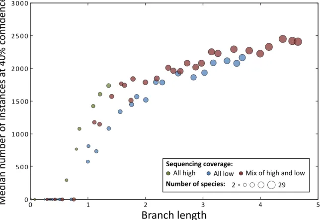
Figure 2-10: Scaling of motif instances using different species subsets. We reran our instance prediction procedure using varying number of species and found that it appears prediction power has not yet saturated. We note that we continued to use the same alignments, simply using only rows corresponding to the species of interest. Consequently, performance strictly on fewer species could be worse because the alignments would not benefit from the intermediate species. The

relative value of low coverage (∼2x) and high coverage (∼8x) is shown.

(Schmidt et al., 2010). When we consider only those binding sites that are also conserved in mouse, we find that the enrichment is dramatically higher (Figure 2-6b).

2.5 Scaling of motif instance prediction

Due to their short length and degeneracy, instance prediction greatly benefits from additional species. Indeed, for the mammals we find an increase in the number of predicted instances as the total branch length of the species considered is increased (Figure 2-10). Further, while for a given branch length using high

(47)

coverage genomes consistently leads to higher sensitivity than using low coverage genomes adding low coverage genomes still significantly improves performance. We also examined the extent to which adding additional species affected the quality of the motif instances in terms of predicting bound regions. We found that while we found many more instances at the same confidence level using more species, the enrichments in experimental datasets is comparable (Figure 2-11). This is consistent with our expectation that additional species gives us higher power for the prediction of motif instances that are likely to be functional, while our confidence measure accurately assesses their quality.

2.6 ChIP vs. motif instances

While there is a correlation between ChIP and comparative motif instances, there are also significant differences. This raises the question of which more accurately predicts motif instances that are likely to be functional. Consequently, we identi-fied regions independent from both ChIP and motif matches that we expect to be associated with likely functional regions bound by a given factor and use these to compare the two.

We expect instances of NF-κB, an important immune regulator, to be prefer-entially located in GM/HUVEC enhancers and in the upstream regions of im-mune response genes. Indeed, we see this trend for both NF-κB motif instances and ChIP bound regions (Figure 2-12). Further, we continue to have an enrich-ment (4.2-fold) for motif instances that do not intersect with the ChIP regions. Moreover, considerably higher enrichment is seen for motifs in the promoters of immune response genes. ChIP regions that have a motif instance are more than two-fold more enriched in these likely functional regions than either of the criteria alone, demonstrating the complementarity of motifs and experimental techniques. We see a similar trends for STAT1 and p53 in enhancers where we expect them to be active (Figure 2-12).

(48)

# instances

4

29 Enrich in bound

4 29 sps

CTCF

ER

Fos

FOXA2

HNF1

HNF4

HNF6

Myc

NF‐κB

NRSF

p53

STAT1

YY1

23,272

28,639

51.3

46.2 2,162

3,720

137.0

206.3 5,937

13,893

34.7

29.9 3,396

6,125

98.9

70.5 6,505

11,436

63.4

64.9 3,052

6,683

30.0

22.3 11,717

22,461

8.1

8.5 1,060

1,650

69.2

73.6 1,461

1,873

35.7

35.0 1,809

2,437

469.4

412.7

0

340

15.0

319

572

22.0

20.0

578

921

223.2

167.8

Figure 2-11: Comparison of motif instances at 40% confidence using only 4 mam-mals (human, mouse, rat, dog) to those found using all 29 mammam-mals. Bars show log ratio of indicated numbers.

(49)

TF Comparison region Targets Enrichment Number of insts

NF‐κB GM/HUVEC enhancers ChIP (GM12878) 28.3 27,873

Conserved mo�f instances 21.4 1,680

ChIP/Mo�f intersec�on 49.2 644

Mo�fs without ChIP 4.2 1,036

NF‐κB Immune response

genes (GO:0006955) ChIP (GM12878)_{Conserved mo�f instances} 3.0_6.3 27,873_1,680

Mo�fs without ChIP 3.1 1,036

STAT1 K562/GM enhancers ChIP (HeLaS3) 6.8 30,046

Conserved mo�f instances 5.8 422

Mo�fs without ChIP 0.0 269

p53 NHEK/HMEC enhancers ChIP (HCT116) 2.3 31,904

Conserved mo�f instances 12.7 193

Mo�fs without ChIP 12.7 154

Figure 2-12: Comparison of ChIP and comparative motif instances (at 40% confi-dence) for predicting regions and genes likely to be bound by a factor. Enhancer regions defined in Ernst et al. (2011). Regions within 2kb of a gene TSS are used as for assessing regulatory enrichment.

(50)

and Mef2) have comparable ability to find muscle genes (as defined in Tomancak et al., 2002), again with the intersection having considerably higher enrichment. Moreover, for the mesodermal repressor Snail, whose binding sites we expect to be avoided near mesodermal genes, we find that particularly true for comparative motif instances. Given that the motif instances have enrichments consistent with those of ChIP, a significant advantage beyond the low cost of the motif instances is their ability to suggest specific regulatory bases — a property we will take advantage of in Chapter 6.

While we see comparable enrichments for motifs and ChIP datasets in these functional defined regions, the sensitivity can differ dramatically between the two. For example, the factors shown in Figure 2-12 have many more peaks than the number of motif instances at 40% confidence. Consequently, when few compara-tive motif instances are available, ChIP may be more appropriate for identifying a broad range of the targets of a factor. However, these results suggest that com-parative motif instances would perform comparably to ChIP when only a small number of confident instances are necessary.

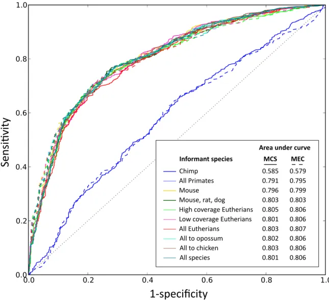
2.7 Comparison to motif discovery

While de novo comparative motif discovery (Cliften et al., 2003; Kellis et al., 2003; Xie et al., 2005; Stark et al., 2007b) and instance prediction are related problems, motif discovery does not generally benefit from additional species as much as mo-tif instance prediction does. Indeed, we have found that a small number of species appropriately placed is sufficient to statistically distinguish real motifs from fake ones (Figure 2-14). This is a consequence of motif discovery methods leveraging statistical over conservation across thousands of matches without needing to pre-dict any individual instances. Moreover, we find that genome-wide conservation scores are highly correlated when computed both when using four species and the entire eutherian tree (Figure 2-15).

Computational regulatory genomics : motifs, networks, and dynamics

Computational Regulatory Genomics:

Motifs, Networks, and Dynamics

by

Pouya Kheradpour

Doctor of Philosophy in Computer Science

at the

MASSACHUSETTS INSTITUTE OF TECHNOLOGY

February 2012

c

Pouya Kheradpour, MMXII. All rights reserved.

The author hereby grants to MIT permission to reproduce and

distribute publicly paper and electronic copies of this thesis

document in whole or in part.

Author . . . .

Department of Electrical Engineering and Computer Science

February 3, 2012

Certified by . . . .

Manolis Kellis

Associate Professor of Computer Science

Thesis Supervisor

Accepted by . . . .

Leslie A. Kolodziejski

Chair of the Committee on Graduate Students

Computational Regulatory Genomics: Motifs, Networks, and

Dynamics

by

Pouya Kheradpour

Abstract

Acknowledgments

Contents

Chapter 1

Introduction

1.1

Motivations

1.2

Relevant biology background

1.2.1

Basics of molecular biology

mRNA

Func�on

Protein

DNA

transla�on

microRNAs

various modiﬁca�ons

Regulated by:

folding

transcrip�on factors

transcrip�on

ma-TF2

TF1

miRNA1

1.2.2

Gene regulation

Protein coding gene

with miRNA binding site

mRNA

RNA Pol II

transcrip�on

Processing by

Dicer

Processing

by Drosha

RNA Pol II

transcrip�on

pre‐miRNA

hairpin

(~70‐nt)

Primary

(pri‐)miRNA

miRNA gene

Cytoplasm

Nucleus

Discarded

miRNA

star

RNA induced silencing

complex (RISC)

mature