Component-based car detection in street scene images

Component-based Car Detection

in Street Scene Images

by

Brian Leung

Submitted to the Department of Electrical Engineering and Computer

Science

in partial fulfillment of the requirements for the degree of

Master of Engineering in Computer Science and Electrical Engineering

at the

MASSACHUSETTS INSTITUTE OF TECHNOLOGY

May 2004

Ln

©

Brian Leung, MMIV. All rights reserved.

The author hereby grants to MIT permission to reproduce and

distribute publicly paper and electronic copies of this thesis and to

grant others the right to do s

Author...

Department of Electrical Engineering a

0. _{MASSACHU ETTS} INSTI E OF TECHNOLOGY

EJUL

20 2004

LIBRARIES

... ...

nd Computer Science

May 20, 2004

Certified by...

Tomaso Poggio

Eugene McDermott Professor

Uh,sis Supervisor

Accepted by ...

.

Arthur C. Smith

Chairman, Department Committee on Graduate Students

Component-based Car Detection

in Street Scene Images

by

Brian Leung

Submitted to the Department of Electrical Engineering and Computer Science on May 20, 2004, in partial fulfillment of the

requirements for the degree of

Master of Engineering in Computer Science and Electrical Engineering

Abstract

Recent studies in object detection have shown that a component-based approach is more resilient to partial occlusions of objects, and more robust to natural pose variations, than the traditional global holistic approach. In this thesis, we consider the task of building a component-based detector in a more difficult domain: cars in natural images of street scenes. We demonstrate reasonable results for two different component-based systems, despite the large inherent variability of cars in these scenes.

First, we present a car classification scheme based on learning similarities to fea-tures extracted by an interest operator. We then compare this system to traditional global approaches that use Support Vector Machines (SVMs). Finally, we present the design and implementation of a system to locate cars based on the detections of human-specified components.

Thesis Supervisor: Tomaso Poggio Title: Eugene McDermott Professor

Acknowledgments

First, I would like to thank Tommy for being such a patient and understanding thesis advisor. His foresight, intuition, and care were instrumental in shaping this work. I want to thank rif for his role as both a teacher and an advisor. He taught me how to dig deeper and provided me with the guidance I needed to get started. I thank: Stan, for his insights and intuition in the subject matter of this thesis. Lior, for his seemingly infinite supply of ideas and new avenues of research to pursue. I must thank Tommy again for letting me work with such great researchers. Lastly, I thank my family whose hard work and sacrifice made this thesis even possible.

If I may, I would also like to take this moment to thank the many great teachers, mentors, managers, advisors, and friends that I have had the pleasure to interact with over the past 5 years.

Much of the work in this thesis is joint work with various members of CBCL. The work in Chapter 3 of this thesis is joint work with Stanley Bileschi and Ryan Rifkin. The work in Chapter 4 is joint work with Lior Wolf.

Contents

1 Introduction

13

2.1.1 Statistical Learning Framework . . . . 20

2.1.2 Feature Spaces . . . . 23

2.1.3 Global Approaches . . . . 24

2.1.4 Component-based Approaches . . . . 24

2.2 Object Detection Framework . . . . 25

2.3 M iscellaneous . . . . 26

3 Hierarchical Car Classifier using an Interest Operator 29 3.1 Interest Operator and SIFT Feature Descriptor . . . . 30

3.2 Keypoint-based Car Detector . . . . 31

3.3 Experiments . . . . 32

3.3.1 D atabases . . . . 32

3.3.2 Global (Non-hierarchical) SVM Classifiers - A survey of feature spaces ... .... . . .. . ... . ... .. . .... . . 34

3.3.3 Keypoint-based Car Detector . . . . 37

4 Component-based Approach 4.1 System Architecture ... 4.1.1 Component Detection . 4.1.2 Component Combination 4.1.3 Car Detection . . . . 4.2 Experiments . . . . 4.2.1 Database . . . . 4.2.2 Component Detectors. . 4.2.3 Component Combination 4.2.4 Car Detection . . . . 4.3 Discussion . . . . Classifiers 5 Conclusion

5.1 Comparison with Prior Work in Car Detection

6 Future Work

6.1 Derivative Work . . . . 6.2 M ore Objects . . . .

6.3 Context and Segmentation . . . .

6.4 Object Identification and Categorization . . . .

43 43 44 47 48 49 49 50 50 51 56 59 60 63 63 64 64 65

. . . .

. . . .

. . . .

. . . .

List of Figures

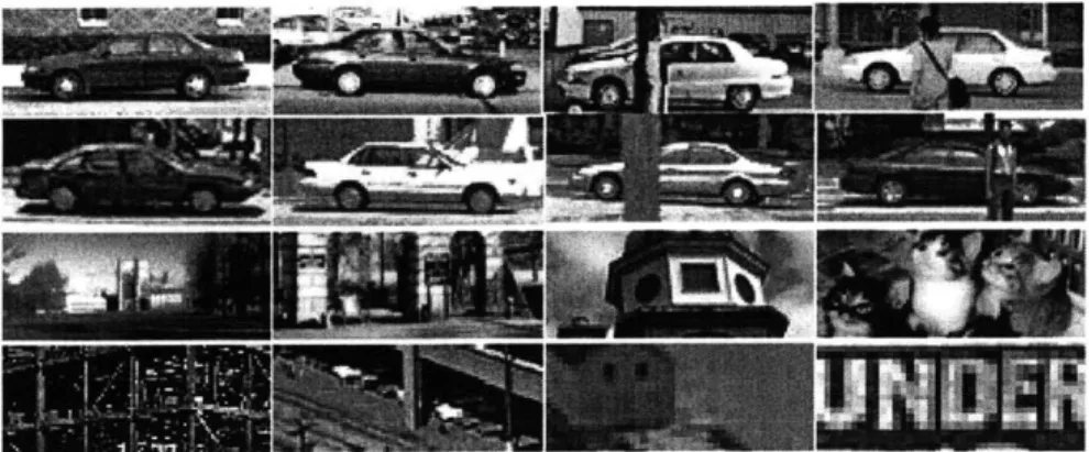
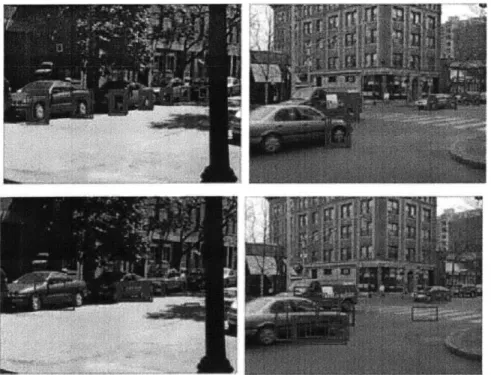
3-1 Examples of cars and non-cars from the training and test set in the Modified UIUC Image Database for Car Detection. All car images are side views of cars where the car is spatially localized in the image. The first and third row are examples of positive and negative training images. The second row contains the crops from the test images of the UIUC Image Database; these images were used as our positive test images. The last row contains examples of negative test images. . . . 33 3-2 Examples of cars and non-cars from the training and test set in the

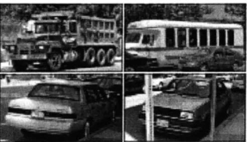
StreetScenes Subset Database. . . . . 33 3-3 Difficult car examples from the StreetScenes Subset database. .... 34 3-4 ROC plot comparing performance on the UIUC Image Database of

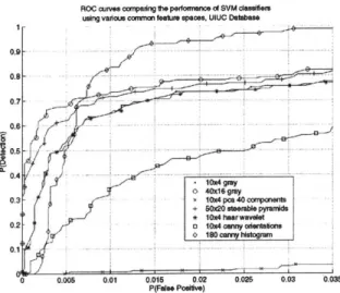
SVM classifiers using various common feature spaces. . . . . 35 3-5 ROC plot comparing performance on the StreetScenes Subset Database

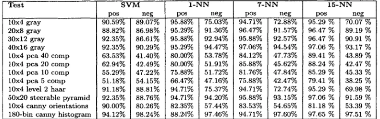
of SVM classifiers using various common feature spaces. . . . . 36 3-6 Error rates on the UIUC Database positive and negative test sets. 170

positive examples, 4183 negative examples in test set. . . . . 37 3-7 Comparison of the Keypoint-based Car Detector to Global SVM

Clas-sifiers on the UIUC Image Database. . . . . 38 3-8 Comparison of the Keypoint-based Car Detector to Global SVM

Clas-sifiers on the StreetScenes Subset Database. . . . . 38 3-9 Performance on the UIUC Image Database of the Keypoint-based Car

3-10 Performance on the StreetScenes Subset Database of the Keypoint-based Car Detector as we vary k, the number of cluster centroids used. 40

3-11 Positive training images from the UIUC database displaying the most expressive keypoints. The size of the keypoint represents the scale at which the keypoint was taken. A keypoint is displayed in red if it is a 'car keypoint'. A keypoint is colored green if it is a 'background keypoint'. . . . . 40

3-12 Comparison of the SIFT Descriptor with a Local Patch Descriptor for the keypoint-based car detector. The experiment was performed on the UIUC Image Database . . . . 41

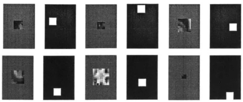
4-1 Examples of patches used as templates and their associated binary spatial mask indicating the region over which a feature is extracted. These regions are chosen to be a square of size 5x5 pixels. The size of the patches range from 3x3 pixels to 14x14 pixels. . . . . 44

4-2 Examples of part detections for wheels and the sidepanel. A threshold is chosen by setting the number of permissible false detections to one false positive for every 106 windows . . . . 47

4-3 Labelings of car images in the Street Scenes Labeled Subset. . . . . . 50

4-4 ROC curves from 4 component classifiers: wheels, roof, sidepanel, windshield. The components are in order with the curve for wheels in the upper left corner and the curve for the windshield in the lower right corner. . . . . 51

4-5 ROC curve comparing performance of three different component com-bination schemes. The worst performance is the system that just uses the maximum value of each component. The next worse curve is the ROC curve for the method that concatenates the maximum value of detection and the position of the maximum detection for each part into one feature vector. The curves on top use the maximum-value-in-subregion approach for varying number of maximum-value-in-subregions. ROC curves are generated from a dataset of cropped cars and non-cars. . . . . 52 4-6 ROC curves comparing system performance on a test set between our

component-based system (solid line) and the baseline global car detec-tor (dashed line). . . . . 53 4-7 Correct Detections . . . . 54 4-8 Difficult examples of cars that were detected correctly. The left side

image has a truck with many wheels that was correctly detected. The right has pictures of the front and back views of cars. These views are not represented well by the three components used in the component detection system. Specifically, the wheels and the sidepanel do not show up in these cars. . . . . 54 4-9 False Detections: found in trees, on walls, on the windshield of a car,

and parts of a store front. . . . . 55 4-10 Interesting Examples of Incorrect Detections: grouping multiple cars

together, a bridge between two cars in a row, off-center detection due to occlusion, multiple partitioned detections for one object. . . . . 56

Chapter 1

Introduction

Our day-to-day lives are abound with instances of object detection. Crossing the street after first checking for cars, recognizing a familiar face, identifying sushi, and finding Waldo in those childhood "Where's Waldo?" picture books are all examples of object detection. We as humans are surprisingly good at it. Unfortunately, building a system that can perform object detection reliably is a dauntingly complicated and difficult computational task. When compared to existing computer vision systems, each one of us can more accurately and more quickly identify instances from many more different classes of objects. More importantly, we can more quickly learn to identify new instances of objects, and new classes of objects. Although a great deal of research has already been performed to advance the field and improve the capability and robustness of object detection systems, we are still many years from closing the performance gap between the human visual system and engineered object detection systems.

The difficulty in object detection is compounded by the high variability in ap-pearance between objects of the same class and the additional variability between instances of the same object due to differences in viewing conditions. Specifically, an object detection system must be able to detect the presence or absence of an object, such as a car, under different illuminations, scales, poses, and under differing amounts of background clutter.

1.1

Problem Statement

Recent studies in object detection have shown that a component-based approach is more resilient to partial occlusions of objects, and more robust to natural pose variations, than the traditional holistic approach. These component-based object detectors are built hierarchically, where simpler detectors first locate components of an object, and a combination classifier makes the final detection with the outputs from each of the component detectors as features. Accurate results have been reported in both face [11, 12, 3] and pedestrian detection [18, 17]. In this thesis, we apply a component-based approach to a more difficult domain: cars in natural images of street scenes. We demonstrate reasonable results for two different component-based systems, despite the large inherent variability of cars in these scenes.

Detecting cars is a considerably more difficult problem than detecting faces or pedestrians. The human face has a simple, semi-rigid structure, where the localization of face components does not vary much between samples. Cars have a semi-rigid structure as well, but that structure will vary more between samples, because their shapes and configurations have been designed with product differentiation in mind.

Besides the intra-class variations due to color, shape, and ornamentation, which similarly plague face and pedestrian detection systems (to a lesser degree), there are other issues that complicate car detection. First, we wish to be able to detect a car irrespective of the view or the out-of-plane rotation. Compared to the other object classes, the car also has more views that are interesting. One major difficulty in object detection is the fact that different views of the same object can look very different, because an image is essentially the projection of a 3D object onto a 2D plane. The face has far fewer degrees of freedom, because only frontal views, side profiles, and any pose in between are of general interest. This restriction reduces the intra-instance variability due to viewing conditions. Usually different classifiers are trained for the different views as was done in [24] to achieve rotation invariance.

Second, the car has many more candidates for components, and only a subset of these components are viewable from any particular perspective. For example, the

tail lights would typically be obscured if the headlights are in plain view and the license plates are usually not viewable from a direct side view. In a component-based detection framework, this suggests that we ought to place more emphasis on the component detection combination algorithm. This situation can be compared to face

or pedestrian detection with large amounts of occlusion.

In this thesis, we explore the selection of object-specific components, the learning of the selected components, and the combination of component detections in order to determine whether or not there is an advantage in building hierarchical classifiers for a broad set of object classes. We expect that this framework works well for classes where an object is comprised of distinct identifiable components or parts and they are arranged in a limited set of well-defined geometric configurations. Although our ultimate goal is generic object class detection, we hope to gain more intuition on the object class detection problem by concentrating on the classification and detection of cars. Our incremental one-object-at-a-time approach toward achieving a "dictionary" of object detectors may also aid researchers in building application-specific object detectors.

1.2

Motivation

Object detection and recognition are necessary components in an artificially-intelligent autonomous system. They provide such systems a context that facilitates interaction with its outside environment. Eventually we expect these artificially-intelligent au-tonomous systems to venture onto the streets of our world, thus requiring detection of objects commonly found on the street. From a systems-perspective, the low-level recognition of objects provides a layer of abstraction to the system, allowing it to perform scene-understanding by manipulating the objects that were detected rather than using the underlying pixel intensities. The need to develop extensible object de-tection frameworks for reliable dede-tection of many different kinds of objects in natural scenes increases as such autonomous systems become more prevalent.

an increase in commercial interest. Academic research has been successfully applied in the areas of law enforcement, surveillance, authentication and access control sys-tems, and computer chip verification processes to name a few. The human face, in particular, has received much attention because of its prominence in visual images and the multitude of emergent applications. The task of identifying generic objects in still images can also greatly enhance the computing experience of the Internet and the World Wide Web. For example, object detection can be applied to labeling and indexing images found on the web, allowing users to manipulate the medium with more sophistication. As the number of real-world applications of object recognition increase, there is a need for accurate recognition systems that can be easily applied to different object classes with fewer constraints on extrinsic imaging parameters, such as pose, illumination, scale, position, etc.

Our long-term goal is toward a system that can accurately locate in an image particular instances from many generic object class. Such a system can serve as a "dictionary of classifiers", usable as a primitive for scene-understanding applications. Success can ultimately be measured by comparing the system's accuracy to that of a human performing the same task.

The direct motivation and an immediate application of the work in this thesis is to facilitate the tedious and error-prone labeling of objects in a database of natural images of street scenes, a database that we can use to study reliable object detection for scene-understanding applications. For this reason, we stress extensibility in terms of applicability to many object classes over the raw accuracy for each individual object class. The database contains images of objects in the 'wild'. This makes the task of object detection even more difficult, as objects may be in any natural pose, illumination, scale, position, etc. Our systems are designed with these multiple degrees of variation in mind.

1.3

Outline of Thesis

Chapter 2 discusses the background required to realize an object detection system. We discuss the object (binary) classifier in a statistical learning framework, survey and evaluate a set of feature spaces, and finally develop the framework in which the classifier is applied to candidate patches in an image. Where relevant we discuss previous work in the field.

In Chapter 3, we present an hierarchical car classifier that outperforms holistic car classifiers in distinguishing between a car patch and a non-car patch. This car classifier combines measures of similarity to diagnostic keypoints, which are local features around points extracted by an interest operator. We then evaluate this system and compare it to holistic classifiers. Finally in Chapter 4, we demonstrate a working system that combines component detections for the car detection task. The components we used were chosen a priori and examples in the database were hand-labeled.

We conclude the thesis in Chapter 5 and discuss future avenues of research in Chapter 6.

Chapter 2

Object Detection

Object detection in an image, the act of finding an instance of an object class in an image, can be viewed as the application of pattern recognition. We first build a classifier that can distinguish between an image patch that belongs to the target object class and one that does not belong to the target object class. We primarily employ Support Vector Machines (SVMs) for classification, but our component-based system in Chapter 4 employs an AdaBoost classifier for the component detections. These classifiers are discussed in Section 2.1.

After we build object classifiers, we search through all windows of the image at various scales, to identify patches belonging to the target object class. We discuss this aspect of object detection in Section 2.2. Outside this chapter, we use the term object

detection for both the classification of a particular window and the task of searching

all such windows with a classifier.

From a systems perspective, it is advantageous to view the object detection task as the application of an object classifier to many windows of an image at different scales. This view essentially decouples the task of building good classifiers from the infrastructure required to actually perform the detection. As suggested in [2], we ought to use the best classifier possible and the best infrastructure.

2.1

Object Classifier

Classifying whether an image patch belongs to a particular object class or not is a pattern recognition task. Specifically, if we are given a feature vector representing an image or a transformation on the image, we would like to be able to classify whether or not the image belongs to the particular object class. As phrased, it becomes a statistical learning problem, where we learn from example images of objects how to distinguish between objects that belong to the target object class and objects that do not belong to the target object class. We learn the discriminative features that separate the two classes, so that when we are given new images, we can determine whether or not it belongs to the target class with a certain level of confidence.

In this framework, there are two choices open to design. The first is the choice of classifier to use. There are many choices that have been shown to work reasonably well, like neural networks, SVMs, and variants of the AdaBoost algorithm to name a few. The second choice is the choice of feature space. Successful systems have been developed using the original gray-scale pixel intensities, gradient images, edge maps, wavelet coefficients, and many others.

In the statistical learning literature, there has been much debate over the choice of classification algorithms. In most cases, it is the choice of features that is important for accurate results. A carefully chosen classification algorithm will give marginal improvements. In the following sections, we give a brief overview of the classifiers used in this paper without much fanfare about its choice. Afterward, we will provide an empirical comparison of different feature spaces for the car classification task in question.

2.1.1

Statistical Learning Framework

Learning is the problem of deriving a predictive function that when given a new observation x can assign the correct label y to the observation with some level of confidence. The function is judged by its ability to generalize to new unseen examples. Supervised learning uses a large training set of examples, a set of (x, y) pairs to derive

this function. We present here an overview of the classification algorithms that we use in this project. A more theoretical introduction to Support Vector Machines can be found in [4, 22]. We use the SvmFu 3.0 implementation of the Support Vector Machine algorithm [21].

Support Vector Machines

Support Vector Machines (SVMs) have found many uses in object detection [11, 18] and have been applied to many other problem domains. SVMs belongs in the class of Tikhonov regularization algorithms, a general approach to finding a function that exhibits both small empirical error and a small norm in a Reproducing Kernel Hilbert Space, K. By choosing the Tikhonov regularization loss function to be the hinge loss,

V(f(x), y) - (1 - yf(x))+ where (k)+ - max(k, 0), we can state the SVM training

problem as

min EZV(f(xi),yi)

+

A11fIIK,

(2.1)

f0ii=1

where f is the number of points in our training set, K is the Kernel Hilbert Space. Af-ter introducing slack variables to deal with the non-differentiable hinge loss function, we can apply the Representer Theorem, suggesting a solution

f*

f*(x) = ZciK(x,xi). (2.2)

i=1

A substitution of the solution f*(x) into the Tikhonov regularization formulation will reduce it to a constrained quadratic programming problem. Introducing a bias term and then solving the quadratic programming problem results in the set of ci and b. A more complete derivation can be found in [22].

Because of the choice of loss function, the solution is often a sparse one, where many of the ci in equation 2.2 are zero. This gives a bound on the complexity of the classifier as well as one on the empirical error. It is this property that allows SVMs to be successful in learning with very few examples within high-dimensional spaces.

In this thesis, we primarily use an SVM formulation with a linear dot product

kernel. With a linear kernel, the solution of equation 2.2 reduces to

f*(x) = w -x, (2.3)

where w is normal vector that specifies the separating hyperplane. We take the sign of the solution in equation 2.3 to be the classification. There are a few considerations that need to be taken care of when a separating hyperplane cannot be found in the feature space. This is primarily related to the choice of C in the SVM formulation. C is the parameter that controls the trade-off between classification accuracy and the norm of the function.

Note that we are specifically concerned with binary SVM classification, however there exist methods to combine binary SVM classifiers for the purpose of multiclass classification. See [23] for an empirical comparison of the many schemes. Additionally, SVMs can be formulated to handle regression problems.

Boosting Algorithm for Classification

Boosting algorithms have been applied successfully in numerous object detection sys-tems [34, 30]. In [34], an object detection framework is built to process images rapidly and with high detection rates. They apply AdaBoost [26] to build an attentional cas-cade of progressively more refined classifiers.

A boosting algorithm additively combines the outputs of weak learners into a strong learner. A strong learner is a classifier that can learn the underlying target function arbitrarily well, given enough training data, while a weak learner is one that can barely perform better than chance, given enough data. AdaBoost is an iterative procedure to construct a strong classifier from several weak classifiers. A typical weak classifier to use is a simple decision or regression stump of the form

where xi is the ith component of the feature vector x, 6 is a threshold, 6 is an indicator function, and a and b are regression parameters to best fit the data. The final classifier is a linear combination of the weak classifiers of the form:

M

H(x)

hi(x),

(2.5)

i=1

where M is the number of rounds of boosting.

An AdaBoost algorithm typically works as follows. We first start off weighting each training data example equally. For each round of boosting, we fit a weak classifier to the weighted data. Then we adaptively adjust the weights on the training data for the next round of boosting to place more emphasis on errors made in the current round. There are a few variants of this algorithm; the differences lie in how the algorithm computes the re-weighting of the training data [8]. In this thesis, we use the Gentle AdaBoost variant described in [8]. It has been shown to work well in object detection applications [30, 14]. AdaBoost has also been found to be resilient to overfitting of data.

2.1.2

Feature Spaces

As mentioned before, a main task of object detection is determining the feature space in which to learn. Various feature spaces have been successfully employed for the tasks of face and pedestrian detection. From experience, it seems that the choice of feature space is heavily dependent on the object class. A feature space that works best for faces may not work well for pedestrians, and vice versa.

For face detection, a comparison of scale pixel values, first derivative of gray-scale images, and wavelets is available in [11); it suggests that gray-gray-scale pixel values are often a good enough choice. On the other hand, haar wavelet coefficients were found to work well in pedestrian detection [17, 18].

In Section 3.3.2, we perform our own comparison of various feature spaces for the task of classifying cropped images of cars and non-cars. On one dataset, we found

between cars and non-cars. On a different data set, the histogram of edge orientations did not perform well at all. From this study, it seems that gray-scale pixels are also

a good enough choice for the class of cars.

[11, 29] also evaluate methods of feature reduction like Principle Component Anal-ysis (PCA) and feature selection based on an ordering of the coefficients of the re-sulting SVM hyperplane specified by w. Other feature selection methods like the one proposed in [36] can also be used.

2.1.3

Global Approaches

Many early face detection systems like that of [19] and [24, 32] employed a holistic approach to the problem of face detection. These approaches take the face as a single unit and perform classification on features generated from the entire face. In these systems, SVMs or neural networks were trained to discriminate between face and non-face images. Rotation invariance was built into the system in [24] by training several neural networks, one for each possible discretized amount of rotation. In [20, 24], improvements were made by using virtual examples to increase the size of the training set. Virtual examples were generated by rotating, translating, or scaling the original faces. Including these virtual examples reduces the sensitivity of the classifier to these variations, which may be present in new test examples. Confusable non-faces have also been bootstrapped into the training set to improve the accuracy of the classifiers.

2.1.4

Component-based Approaches

Recently, component-based approaches to object detection like the ones in [18, 12, 3, 37] have become more fashionable. The intuitive motivation behind a component-based approach is that each part of an object should be less sensitive to changes in illumination, pose, and rotation than the object as a whole. Component-based systems can also be engineered to deal with partial occlusion by clutter or strong directional lighting. Furthermore, they can leverage the geometric information and constraints in the configurations of the components. Empirically, they have been

shown to produce better accuracy than global, holistic approaches [3].

A typical component-based object detection architecture involves selecting compo-nents to be trained, selecting a feature description for each component, and combining detected components for the final object classification. In selecting the components to be trained, systems like [11] use the typical facial features, such as eyes, the nose, and the mouth. The system has then been improved in [12] to select salient features automatically using a region-growing algorithm with a statistical bound. In [35, 6], in-terest operators were employed to select keypoints in images, and a generative model is learned on a selected subset of these keypoints to explain the data. Besides the choice of components, systems differ in their choice of feature description. Gray-scale pixel value features can be used like in [3]. The system in [28] extracts features from the wavelet decomposition of images to build a histogram-based classifier.

Once part examples have been detected in an image, component-based object detection systems will employ a second-layer classifier to determine whether or not the parts taken as a whole belong to a member of the object class or not. Several approaches can be taken. Some approaches perform a likelihood ratio test that deter-mines whether a given configuration of detected parts is more likely to have stemmed from a member of the object class or not [3, 6]. Others like [37] search in a set of pre-viously seen configurations for the best geometrically consistent subset of extracted parts from the image. In [12], an SVM is trained to decide whether or not the set of positions and confidences of each part is likely to have come from a face. This SVM

is then evaluated on the features from the best detections for each component.

2.2

Object Detection Framework

The final step of object detection in images is to apply the learned classifier to all the potential windows of the image at different scales. Objects are considered detected in a window if the classifier has a high enough activation value. In [1], they the coin the term classifier activation map for the outputs of the classifier on windows of the image.

Objects in images may appear at different scales depending on the depth of the object with respect to the camera. Therefore it is important to search the image at different scales in order to detect all objects. To keep the number of features of the classifier fixed, we iteratively scale the image by a specified amount.

In object detection, the choice that impacts the visible results of detection most is the threshold at which the classifier operates. Usually, our classifiers are too per-missive in what they classify as members of the target object class. This is because our training set does not reflect well the actual probability distribution of objects, over-stressing the presence of positive instances of the target class. We alleviate this by choosing an operating point on a Receiver Operator Characteristic (ROC) plot in the region of low false positives. We choose an operating point that satisfies our requirements against false positives; it is usually a choice based on the number of inspected windows.

Another important issue to resolve is the multiple detections that may occur for the same object. These multiple detections may also occur across a few scales. In many respects all these detections are correct, but a single detection is often required for some applications. A few methods have been employed to reduce the multiplicity of correct detections. The most common method partitions the detected windows into disjoint, non-overlapping groups, and the best (highest activating) detection in each group is used. Problems arise here when we have multiple cars very close to each other and the non-overlapping constraint may be too strong. Another approach is to take, as the best location, the maximum activation in a specified neighborhood of potential locations across multiple scales. If two locally maximal activations occur in close proximity to each other but are outside of each others neighborhood, then both activations are considered detections.

2.3

Miscellaneous

In computer vision, a natural extension of object detection is to the task of object identification, where an instance of a particular object is classified into one of many

smaller subclass. In particular for faces, it is often useful to determine the identity of the face wherever a face has been detected. Although we do not address the identification aspect of recognition in this paper, we can very easily generalize binary classifiers for multiclass classification in order to perform such object identification. In general, one-versus-all has been shown to work well for many multiclass classification

Chapter 3

Hierarchical Car Classifier using an

Interest Operator

In the previous chapter, we discussed a few systems suggesting that accurate and powerful object detectors can be built in a hierarchical component-based fashion. In this chapter, we plan to demonstrate that this hierarchical structure is advantageous for object detection in images with cars. We discuss a hierarchical car classifier based on salient features extracted by an interest operator. The classifier operates by first locating keypoints in the test image with an interest operator. These keypoints are then compared against a corpus of car-specific keypoints learned from the training data. The resulting similarity vector is input into an SVM classifier. We then compare the performance of this classifier to non-hierarchical classifiers. In this chapter, we view the keypoints in our corpus of car-specific keypoints as components of cars. The technical and philosophical validity of this claim is open to debate. Nevertheless, we are able to show that this hierarchical "component-based" approach indeed works well for cars.

3.1

Interest Operator and SIFT Feature

Descrip-tor

Extracting distinctive and invariant features quickly from images is an important task for a hierarchical object detection system. It was decided early in the development of this system to use the interest operator discussed in [15] to make this process rapid and robust. Other options were to use those operators described in [7, 9]. The Lowe Interest Operator detects interesting points or keypoints by locating extrema in

D(x, y, a) = (G(x, y, ku)

-

G(x, y, a))

*

I(x, y),

(3.1)

where I(x,y) is the input image, and G(x, y, or) is the variable scale gaussian,

G(x, y,

or)

1

)/2,2. (3.2)

27ro

Each interest point is parameterized by not only the x, y, and scale, but also a dom-inant orientation computed from the neighborhood of D(x, y, o). These parameters impose a 2D coordinate system, providing invariance to translation, scale, and rota-tion [16].

At each keypoint we record the Scale Invariant Feature Transform (SIFT) of the image. The SIFT feature descriptor is designed to be invariant to changes in illu-mination and changes due to 3D viewpoint. These invariances address issues that often plague object detection systems. The computation of the descriptor involves first computing the gradient image of magnitudes and orientations and then dividing a local region around the keypoint into 4x4 sample regions. An orientation histogram with 8 orientation bins is created for each of the regions, where each gradient image pixel contributes its gradient magnitude into the histogram entry (keyed by the gra-dient orientation). Care is taken to avoid boundary effects and effects due to small changes in keypoint location. A threshold is used to limit the contribution of large gradient magnitudes in each histogram entry. This step coupled with renormalization

is performed to reduce the effects of illumination changes. The final result is a 128 dimensional feature vector shown to work very well for object detection tasks. Details are available in [16].

It has been shown empirically [15, 5] that this combination of keypoint detector and image feature works well for object detection.

3.2

Keypoint-based Car Detector

Our goal is to construct a hierarchical car detector by automatically learning car-specific features and then learning a combination classifier. We chose to center our features on the keypoint detections returned by the algorithm described in [15], be-cause they are robust, computationally efficient, and invariant to a number of common image transforms. We take the following approach. First we extract keypoints from car images in our training set. Each keypoint is a 128-dimensional vector representing a 4x4 array of orientation histograms with 8 bins in each histogram. These keypoints may come from an actual car or from the background in a car training image. We cluster the keypoints into a fixed number, k, of clusters, using k-means clustering. Let this set of cluster centroids be the set K, and let K denote the jth cluster centroid. Our initial hope was that these clusters would represent semantic car parts. The next step in training a classifier is representing the training data in terms of the expression strength of these parts.

In order to train an SVM classifier, we must be able to convert the image, I, from the training set into a fixed-length feature vector, V. Let T be the set of keypoints extracted from image

I.

Vj(j)

=

minIKj

-

rnI

(3.3)

rET

Our fixed-length feature vector is now a k-dimensional vector of distances between clusters from the training data and keypoints from the image. In general, since there may be more clusters than there are keypoints in an image, a particular keypoint may

be associated with more than one keypoint cluster.

Intuitively, we expect that car images will have smaller distances to many of the clusters, and non-car images will have larger distances. However, we do not expect this to be a hard rule because we allow background keypoints into the clustering procedure. We do this to avoid manual labeling every keypoint as coming from a car or from the background.

With the described feature representation, we are able to train SVM classifiers. The SVM is trained on positive and negative examples - the positive examples are the same car images from which we extracted car keypoints for clustering 1.

In order to classify a novel image, Z, as a car or a non-car, we first extract keypoints from it. We then calculate the Vz as before. This vector of minimum distances is then passed to the SVM for classification. This process is repeated for each image in the test database. By sweeping over the SVM threshold we can generate an ROC curve, enabling us to compare system performance to other methods. Using these measures, we can examine the effect of free parameters in the system design.

There are numerous free variables in our approach. The keypoint format depends on the number of scales, orientations, and histogram bins. We chose to keep the parameters at the default values suggested by [15]. These values are known to work well for detecting specific objects. We address the parameter k, the number of clusters, in our experiments.

3.3

Experiments

3.3.1

Databases

Modified UIUC Image Database for Car Detection

This database is constructed from the UIUC Image Database for Car Detection

[1].

The UIUC Image Database has a training set with 550 side views of cars and 500

'We showed experimentally that the potential system performance improvement from splitting the training set into two subsets for the purposes of clustering car keypoints and training the SVM classifier was offset entirely by the loss in performance due to less data for training.

Figure 3-1: Examples of cars and non-cars from the training and test set in the

Modified UIUC Image Database for Car Detection. All car images are side views

of cars where the car is spatially localized in the image. The first and third row are

examples of positive and negative training images. The second row contains the crops

from the test images of the UIUC Image Database; these images were used as our

positive test images. The last row contains examples of negative test images.

Figure 3-2: Examples of cars and non-cars from the training and test set in the

StreetScenes Subset Database.

non-car images. Each of these gray scale images are 40 x 100. The cars are roughly

of the same build and at the same position, and are subject to possible occlusion and

differences in illumination. We used this training set unmodified. The provided test

set contains cars to be located in images with a large amount of background. For our

purposes, we cropped out the first car from each of the test images to serve as our

positive test set and provided our own set of negative examples. In total, we have

170 side views of cars and 4183 non-cars for the test set. See Figure 3-1 for examples

Figure 3-3: Difficult car examples from the StreetScenes Subset database.

StreetScenes Subset Database

The StreetScenes database contains high resolution (up to 768 x 1024) images of cars

in a natural environment. The database contains cars, trucks, and buses in many

poses, different degrees of occlusion, as well as variations in illumination. In order to

simplify the problem, we have decided to concentrate on side views of cars. We have

performed semi-automated sorting of the cars in the database by pose in order to

extract the side views of cars. We also extract non-cars from the StreetScenes images

with a similar distribution in sizes. All images are converted into gray scale, extracted

at a fixed aspect ratio, and finally scaled down to a fixed image size. Figure 3-2 shows

examples of images from this database. Our training database contains 350 images

of cars and 4000 images of non-cars. The test database contains 149 images of cars

and 4059 images of non-cars.

Car detection on the StreetScenes database is a considerably more difficult task

than on the UIUC Image Database. Because the side views of cars were

semi-automatically extracted to improve the generality of our methods, errors did occur

as shown in Figure 3-3. Also, the StreetScenes Subset database contains images of

bulldozers and buses, making the classification task difficult.

3.3.2

Global (Non-hierarchical) SVM Classifiers

-

A survey

of feature spaces

For comparison purposes, we perform the learning task on these databases using

canonical statistical learning machines, vis. SVM and k-Nearest Neighbor technique.

ROC usi v oarrne rng to pefonence d SVM dassiffem

classusifiers cmni sar etue spaes, UIUC Des. bm

0.e -. . . . .

0.7-0

~ ~~~~

Figur

3-4: ROpltcmaig efrac

nte

U ImageDataase f SV

We explored system performance using various common feature spaces and a few

novel ones. ROC curves comparing results of different global (non-hierarchical) SVM

classifiers are provided in Figures 3-4 and 3-5. All the ROC plots concentrate in

the low false positive region, because this is the region believed to be important

for the application of car detection in images. All generalizations made in the low

false positive region extends to the high false positive region unless otherwise stated.

Table 3-6 gives error rates comparing SVM performance to k-Nearest Neighbors for

the UIUC Image Database.

The first feature space we explored was the original gray pixel intensities. We

applied the following pre-processing steps. First, each gray scale image is scaled down

to a common size. We vary this to measure the effect on performance. Histogram

equalization is then performed on each image individually to remove variations in

image brightness and contrast.

In [31, 12], it was found that by using Principle Component Analysis (PCA) the

dimensionality of the data could be reduced, while preserving system performance, or

possibly even improving it. Along with gray scale features, we tested PCA features

in this stage of the experiment. We tried running the experiment with 5,10, 20, and

40 principle components.

ROC c-rves ondtpg ft perfoance o SVM ttas btlDbs ufing vaious cmn fe a spacs, Sreetscenes S tu .eetsbas.

o lexiOgasy

0.9 ... x 3WxOgray

+ d es 4 conrreaf t h

0 .8n rln sferable

a 94hcaerw~avl

to inclue was a 80-bin hstogram f the Manyaedge rientatnsmauestec

0.7 ... ....

-I

0 0.006 0.01 0.016 002 0026 0.03 0036

P(Fw1u Post"v)

Figure 3-5:

plot comparing performance on

of SVM classifiers using various common feature spaces.

Additional features tested include haar wavelets, and correlations with an

over-complete bank of steerable filters. We also tried the local canny edge orientation at

each pixel as a feature space. Perhaps the most complicated feature space we chose

to include was a 180-bin histogram of the canny edge orientations, measured at each

pixel.

The ROC curves in Figure 3-4 and 3-5 suggest that the gray-scale pixel intensities

perform better than the other features under comparison for these particular tasks.

We also see that the StreetScenes Subset Database is considerably more difficult than

the UJUC Database.

For the sake of comparing different feature spaces, we provide Table 3-6, the test

set error rates on the UIUC Database of the best SVM classifiers and the best

k-Nearest Neighbor classifiers for each feature space. Although ROC curves are more

useful for image detection applications, we are not able to generate meaningful curves

for the k-Nearest Neighbor classifiers. Nevertheless, we provide this table as part of

the survey of the effectiveness of each feature space. The error rates for the SVMs are

points on the ROC curves of Figure 3-4. Rom the table, we see that at the chosen

operating point, gray value pixels and canny histogram generally work about equally

well, and all other features performed worse.

Test SVM 1-NN 7-NN 15-NN

pos neg pos neg pos neg pos neg

10x4 gray 90.59% 89.07% 95.88% 75.03% 94.71% 72.88% 95.29 % 70.07 % 20x8 gray 88.82% 86.98% 95.29% 91.36% 96.47% 91.57% 96.47 % 89.19 % 30x12 gray 92.35% 86.61% 95.88% 92.94% 95.88% 92.57% 96.47 % 90.91 % 40x16 gray 92.35% 90.29% 95.29% 94.47% 97.06% 94.54% 97.06 % 93.17 % 10x4 pca 40 comp 63.53% 41.40% 80.00% 53.78% 84.12% 47.73% 89.41 % 43.89 % 10x4 pca 20 comp 62.94% 42.49% 80.00% 51.91% 85.88% 45.62% 88.24 % 42.47 % 10x4 pca 10 comp 55.29% 47.22% 75.88% 51.72% 81.76% 47.84% 85.29 % 45.33 % 10x4 pca 5 comp 51.18% 54.15% 66.47% 47.16% 75.88% 42.47% 79.41 % 38.25 % 10x4 level 2 haar 91.18% 88.81% 94.71% 75.37% 94.71% 72.74% 95.29 % 69.98 % 50x20 steerable pyramid 92.35% 88.76% 94.71% 94.20% 95.88% 93.15% 97.06 % 91.59 % 10x4 canny orientations 90.00% 80.26% 82.35% 57.44% 83.53% 54.65% 81.18 % 53.39 %

180-bin canny histogram 94.12% 98.24% 88.24% 97.46% 94.71% 97.60% 97.65 % 97.51 %

Figure 3-6: Error rates on the UIUC Database positive and negative test sets. 170 positive examples, 4183 negative examples in test set.

3.3.3

Keypoint-based Car Detector

In this section, we show results from various experiments we performed in arriving at our current system. We show that our system outperforms our best global SVMs on the databases used in our experiments.

Comparison to Global SVMs.

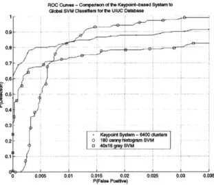
In Figures 3-7 and 3-8, we compare our system using 6400 clusters of car keypoints to our best global SVMs for the two databases. These figures show that our classifier using the local SIFT descriptors at detected keypoints outperforms the best global SVM classifiers in the low false positive region. Only the global histogram of canny orientations on the UIUC Image Database beats our system in the high false pos-itive region of the ROC curve, a region that is not particularly interesting for the application of object detection in images. Additionally, the poor performance of the global histogram of canny orientations on the Street Scenes Subset Database seems to indicate that this particular feature space is highly sensitive to the particular learning task at hand.

Experiments with the Number of Clusters.

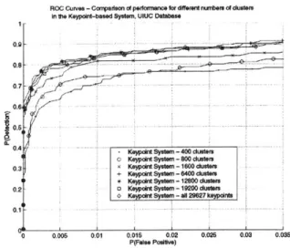
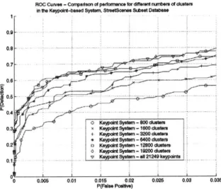
We show in Figures 3-9 and 3-10 that performance generally tends to improve as we increase the number of clusters of car keypoints. There is typically diminishing marginal returns as we increase the number of clusters. On both databases, using

ROC Curves -Compaison of the Keypant-based System to

Global SVM Clasdtem for e UIUC Database

0.8

-S-m-4-s-0.7 - --. --. .

0 .6 - -- - - ---

--0.6 --

-0.3

----Keypoint Systemn -6400 duster

0.2o- 0 tiDcsrsW h gr SVM -13 4(Sl Way SVM

0 0.0 0.01 0015 0.02 0.0 0.03 0.03

P(FW, Positive)

Figure 3-7: Comparison of the Keypoint-based Car Detector to Global SVM

Classi-fiers on the UIUC Image Database.

ROC Curves -Comparison of ie Keypoint-based System to Gobal SVM Clasilers for the StreetScenes Subset Database

SKeypdnt System -8400 clusters

o ltocsnytristogramSVM 0.-- E- 1O s SVM 0.8 . . . . . ... 0.7 - .. .. .. . 0.8 - -0.5 - - - - -. 0.4 -- -.--.-.-.- -0.3 0.2-0,1 0;0 0005 0.01 0.015 0.02 0.02 0.03 0.036 P(Fstse Positive)

Figure 3-8: Comparison of the Keypoint-based Car Detector to Global SVM

Classi-fiers on the StreetScenes Subset Database.

ROC Curves -Comrparison of prteernence for dfferstnumbers df dusters

in Ihe Keypolnt-besed System. UIUC Dstabese

1 - - .. ... . . . . .

0.8 - -....- Sysem- . 4t. us

0.7 6

0 . --. --. ..-. .-. .-..

-o-Keypdt System - -00 -usters

t Keybnt System - 800 dusters

the~~~~~. increase opttoa Syte lotwhwhi dminatdb; h itnecluain

b Keypoint System -12800 dusters

0 G Keypoint System - duste m u2b

0not se

anpr improemen -n Ierformance

o Koi ydnttSystem -an rN67a ydr k

0 0.006 0.01 0.016 002 0.026 0.00 0.00

P(FWSG PosOe)

Figure 3-9: Performance on the UIUC Image Database of the Keypoint-based Car

Detector as we vary k, the number of cluster centroids used.

any more than 6400 clusters does not achieve enough performance gain to warrant

the increase in computational cost, which is dominated by the distance calculations

between keypoint clusters and the keypoints in a test image.

We also experimented with the use of the more powerful Gaussian Mixture Models

(GMMs) instead of k-Means clustering. With the same number, k, of clusters, we did

not see an improvement in performance.

Experiments using all car keypoints and random car keypoints

Because performance seemed to improve as we increased the number of clusters, we

tried using every car keypoint as a cluster centroid. The performance of using all car

keypoints is in general very close to the performance when using greater than 6400

clusters of keypoints. Additionally, we explored the expressiveness of each

individ-ual keypoint in car classification. In Figure 3-11, we provide training images with

keypoints corresponding to negative SVM weights highlighted in red and keypoints

corresponding to positive SVM weights in green. Strong expression of a red keypoint

(a small distance to that keypoint) indicates the presence of a car, whereas the strong

expression of a green keypoint indicates the presence of background. In the training

images, keypoints close to the wheels tend to be colored red. This indicates that if a

ROC Curves -Cormparison of perfonwnce for dffert rubers dF dusters

In 1i. Kyp1dnt-bosed System, StrestSoner Subset Datebese

0

. - -. - -...

-

0.6-o.~~ Keypdint

~

Figure 3-10: Performance on the StreetScenes Subset Database of the Keypoint-based

Car Detector as we vary k, the number of cluster centroids used.

Figure 3-11: Positive training images from the UIUC database displaying the most

expressive keypoints. The size of the keypoint represents the scale at which the

keypoint was taken. A keypoint is displayed in red if it is a 'car keypoint'. A keypoint

is colored green if it is a 'background keypoint'.

keypoint in a novel image is similar to a wheel keypoint, then it is more likely for the

image to be of a car.

We also tried using random subsets of the set of all car keypoints instead of the

cluster centroids. With randomly selected keypoints, accuracy still tends to improve

with increasing number of keypoints; however, accuracy becomes highly dependent

on the random selection of keypoints. This randomness in the selection of keypoints

makes it harder to make any conclusions whether it is better or worse than using

clusters of keypoints.

ROC uies - Conrarsn n d ". pedoanianoe:

Srr Decpor Local Pat Deaclpor

0.98.... .

0.8- .

0.7-0.6

the keypoint-based car detector. The experiment was performed on the UIUC Image

Database.

Local Patch Descriptors vs SIFT Descriptor.

Instead of using the SIFT descriptor, we tried using a local gray pixel descriptor at

the scale of the keypoint extraction. In other words, we extract an image patch of

uniform resolution at the scale of the detected keypoint and record it as our keypoint

feature. We see in Figure 3-12 that the SIFT descriptor performs better than the

local patch descriptors. These arrays of histograms of orientation features seem to

better represent the differences between cars and non-cars.

3.4

Discussion

In this chapter, we have outlined the architecture of a hierarchical car detection

al-gorithm, explored how the performance of this classifier is dependent on variations in

the architecture, and compared the accuracy of the system to that of non-hierarchical

global SVMs trained on the same data. This exploratory study showed that by first

extracting an appropriate high-level feature representation of the data, and

subse-quently training a classifier on the expression of these features, performance can be

boosted. One question the reader may ask is whether or not this system is truly

a part-based car detector. For certain the SIFT features learned from the data are diagnostic for cars, as evidenced by the gain in performance over SVMs trained on other reasonable features. Also the SIFT features are spatially constrained; data from the image is only inspected at or near the keypoint returned by the interest operator. While the clusters we extract in the k-means step represent spatially constrained car specific features, they do not necessarily correspond to what a human would consider as a semantic car part 2.

While the performance of our system is better than that of the best global (non-hierarchical) SVM technique we implemented, it is also considerably more complicated in structure. One might ask if the additional performance is worth the cost. What we have seen empirically is that: while a simple SVM and our technique might do equally well at detecting a car that is very similar to the majority of the training database, our method has the advantage when abnormal conditions, such as a partial occlusion or a strong lighting condition, cause part of the car to look dissimilar to what is expected.

One unexpected result in the course of this experiment was that in general it is better to use as many clusters as possible, almost all the way out to the extreme where every keypoint from the training database is itself its own cluster. In this way our system bears some similarity to a fragmented nearest neighbor technique. Whereas in nearest neighbor classification a test image is compared via a distance metric to every car and non car image in the training data, in our technique every interesting car point is compared to every keypoint from the training data.

In implementing this system, we did not utilize geometrical constraints as is usu-ally done when building a component-based detection system. Early experiments have shown that including the location does indeed provide additional improvements, but further work must be done to investigate the best way to incorporate this information into the system.

2

Some clusters regularly locate the wheel of the car, in this case we would consider the cluster to be a semantic car part

Chapter 4

Component-based Approach

In this chapter, we present a component-based object detection system using pre-selected and manually labeled components. The system is very similar in design to other component-based systems in face and pedestrian detection [12, 18]. For the component detectors, we choose to use the features proposed by [30]. These features were chosen for their computational efficiency and ease of implementation. The full system architecture is discussed in the next section with experiments and conclusions to follow.

4.1

System Architecture

We propose a two-tiered system, where we first detect car parts and then combine these component detections to make the final car detection. We choose car parts that we believe are salient. These parts include: wheels, headlights, taillights, the roof, the back bumper, rear view mirrors, the windshield, and the "sidepanel", a rectangular region between the wheels that includes the shadow underneath the car and lower half of the car doors. Classifiers are learned for each of these parts as described in Section 4.1.1. In Section 4.1.2, we discuss how the part detections are used to train a top-layer car classifier.