A Computer Simulation Model Suite for the Analysis of
All Optical Networks
by
Gregory S. Campbell
Submitted to the Department of Electrical Engineering and Computer
Science
in partial fulfillment of the requirements for the degrees of
Bachelor of Science in Electrical Science and Engineering and
Master of Engineering in Electrical Engineering and Computer Science
at the
MASSACHUSETTS INSTITUTE OF TECHNOLOGY
May 1995
Copyright 1995 Gregory S. Campbell. All rights reserved.
The author hereby grants to MIT permission to reproduce and to distribute
publicly paper and electronic copies of this thesis document in whole or in
part, and to grant others/the ri/hyfo do so.
A uthor ... ~
.
...
_"'"..
.
C.
...
7 " "... ...
· epfment of Electcal Egneering and Computer
Science
/
., / ~ ,/?
May
26,
1995
Certified
by
...
. ..
..
...
,...
Steven G. Finn
Principal Research Scientist
\ .
t
~
.
A,
Thesis Supervisor
Accepted by ...
...;...N .. I. ....
.
...
F.R. Morgenthaler
A Computer Simulation Model Suite for the Analysis
of All Optical Networks
by
Gregory S. Campbell
Submitted to the Department of Electrical Engineering and Computer Science
on May 12, 1995, in partial fulfillment of the requirements for the degrees of
Bachelor of Science in Electrical Science and Engineering and
Master of Engineering in Electrical Engineering and Computer Science
Abstract
In this thesis a suite of models has been developed for the simulation of All Optical
Net-works (AONs) in the OPNET simulation tool. The models are based on the propagation of
pulses through the AON. Pulses are modeled as complex pulse envelopes on a central
fre-quency carrier. As pulses propagate through the network, optical components transform
them and delay them appropriately. Probes can be inserted to view the pulses at specific
points in the network. This knowledge can help an AON engineer make informed
deci-sions about AON design thereby allowing him to more rapidly test possible network
con-figurations.
Thesis Supervisor: Steven G. Finn
Acknowledgments
I would first like to thank Dr. Steven Finn for both his technical and personal inspiration,
guidance and understanding in helping me produce this work. Without his help this thesis
would never have been possible.
I would also like to thank Dr. Roe Hemenway for introducing me to the wonders of
non-linear optics, and helping me understand the dynamics of optical components. This thesis
is much greater thanks to his inspiration.
My parents and family receive my greatest gratitude for helping me come to M.I.T. and
supporting me in all my endeavors. Without them, none of this would have been possible.
Contents
1 Introduction ...
1.1 Background ...
1.2 AON Model Suite Objectives
2 Simulation Concepts ...
2.1 OPNET Concepts ...
2.1.1 Packets ...
2.1.2 Links ...
2.1.3 Nodes...
2.1.4 Processes ...
2.2 Probing and Analysis ....
2.3 A Simple AON Example
3 Simulation Structure ...
3.1 Simulation Global Variables
3.2 Pulse Structure ...
3.3 Noise Structure ...
3.4 Ports and Port Structures ..
3.5 Simulation Flow ...
4 Component Models ...
4.1 Transmitter ...
4.2 Optical Fiber...
4.2.1 Fiber Parameters
4.2.2 Propagation Delay
4.2.3 Split-Step Fourier
4.2.4 Linear Effects...
4.2.5
4.2.6
Non-Linear effects c
Non-Linear effects c
4.3 Fused Biconical Coupler ...
4.4 Star Coupler ...
4.5 Optical Amplifier ...
4.6 ASE Filter ...
4.7 Fiber Fabry-Perot Filter ...
4.8 Mach-Zehnder Filter...
4.9 Wavelength Division (De)Mu
4.10 Wavelength Router ...
4.11 Probe ...
4.12 Receiver ...
5 Simulation Results ...
5.1 Fiber Model ...
5.1.1 Dispersion in Linear
...
17
...
17
.. .. ... .. .. .. .. .. .. .. .. .. .. .. .. ... .. 18
...
19
...
19
...
21
...
21
...
21
...
22
...
22
...
23
...
25
ethod... 47
...
27
...
29
...
4930
...
34
tipee...
37
...
39
...
44
...
45
...
47
lethod ...
47
... ...
4 8
caused by the Pulse ...
48
caused by Pulses at other Frequencies ...
49
.. . ... . .. . .. .. .. .. .. .. . .. .. .. .. .. .. .. 5 1
...
54
...
56
...
.. .. ... .. .. .. .. . ... . .. .. .. .. ... .. . 5 8
...
60
... ... 63
ltiplexer ...
66
...
68
... ... .. . .. .. . ... .. . .. .. ... . .. .. ... .. 7 1
...
7 3
...
...
...
75
76
...
76
...
...
...
...
...
...
...
...
N5.2 Filters ...
5.2.1 Fabry-Perot Filter ...
5.2.2 Mach-Zehnder Filter
5.3 Fused Biconical Coupler ...
...
83
...
83
...
86
...
89
6 Conclusion
...
...
93
Appendix A Component Proci
A.1 aon_xmt0 ...
A.2 aon_xmtseq ....
A.3 aon_xmt0_sech...
A.4 aon_xmt_sechseq
A.5 aon_fib ...
A.6 aon_fbc...
A.7 aon_stc ...
A.8 aon_amp...
A.9 aon_ase...
A. 10 aonfabry ...
A.11 aon_mzf ...
A.12 aon_wdm ...
A.13 aon_rou...
A. 14 aon_probe...
A.15 aon_rcv...
ess Model Reports ...
. . . . . . . .. . . . .. . ... ... *... ... e... ... e...e.... ... *...e.*...ee... ... e..e...e....e....e. ... *..ee..ee....ee...ee ... ... ,.e...*....e..e. .. e....e....e....e.... ... ......
95
...
96
...
98
...
101
...
103
...
106
...
110
...
113
...
117
...
121
...
124
...
127
...
130
...
134
...
138
...
141
Appendix B Supporting Code ...
B.1 Transmitter Support Code ...
aon_xmt.ex.h
.
.
aon_xmt.ex.c
.
.
B.2 Optical Fiber Support Code ....
aon_fib.ex.h
aon_fib.ex.c
B.3 Fused Biconical Coupler Support
aon_fbc.ex.h
aon_fbc.ex.c
B.4 Star Coupler Support Code ....
aon_stc.ex.h
.
.
aon_stc.ex.c
.
.
B.5 Optical Amplifier Support Code
aon_amp.ex.h
...
... ...Code
...
... e...*....e.. ... e..e.,.ee... ... . . . . . . . . , . . . ..... 145
.... 146
·. 146 ·. 146.... 148
·
. 148
·
. 150
.... 164
·. 164 ·. 164.... 167
. 167
. 167
....
169
·. 169...
. . . .
. . . . .
. .
. . .
. .
. .
. . .
. .
. .
. . .
. .
. .
. . . . .
. .
B.8 Mach-Zehnder Filter Support Code ...
aon_mzf.
ex.
h
aon_mzf.ex.c
B.9 Wavelength Division (De)Multiplexer Sup
aon_wdm.ex.h
.
.
.
.
aon_wdm.ex.c
.
.
.
.
B.10 Wavelength Router Support Code ...
aon_rou.ex.h
.
.
.
.
aon_rou.ex.c
.
.
.
.
B. 11 Receiver and Probe Support Code ...
aon_rcv.ex.h
.
.
.
.
aon_rcv. ex.
c
.
.
.
.
B. 12 Complex Mathematics Support Code
cma
th
.
ex
.h
cma
th.
ex.
c
B. 13 Linear Transfer Function Support Code .
aon_lin.ex.h
.
.
.
.
aon_lin.
ex.
c
B. 14 Pipeline Stages
...
aon_ps
.
ex.
h
aon_propdel
.ps.
c
.
aon_proprcv.
ps.
c
.
aon_txdel
.ps
. c
.
aon_
txrcv.
ps.
c
.
.
.
port Code
....
.
.
... ...
.
.
... ..* .
. . . .
. .
.
.
.
.
....
.
.
. .
.
. .
.
. .
.
.
.
.
.
... ... 178... 178
...
180
... ... 180...
180
...
182
... ... 182 ... ... 182...
184
... ... 184 ... ... 184...
188
... ... 188 ... ... 188...
193
...
193
... .... 193...
195
... ... 195 ... ... 195 ... ... 197 ... ... 198Appendix C Usage Comments 201
...
199
178
List of Figures
Figure 2-1: Network level model of a metropolitan area All Optical Network ...
19
Figure 2-2: Node level model of a FBC node. Packets enter the node through point to point
receivers and exit the node through point-to-point transmitters. The components in
the node send packets to each other through packet streams. ...
20
Figure 2-3: Process level model of a simple FSM containing one forced state (init) and one
unforced state (steady). ...
21
Figure 2-4: Simple AON Example to demonstrate how the AON Model Suite and OPNET
work together to simulate an All Optical Network ...
24
Figure 3-1: The pulse shape is defined by complex samples over a span of AonI_Duration
seconds. Here, AonI_Nu = 5 and AonI_Duration = 300 ps. ...
28
Figure 3-2: Mach-Zehnder Filter port layout ...
30
Figure 3-3: Flow diagram for linear component ...
34
Figure 3-4: Flow diagram for non-linear component ...
35
Figure 4-1: AON Transmitter icon and port layout. Incoming packets on port 0 are
discard-ed ...
39
Figure 4-2: Gaussian pulse amplitude (m = 1, to = 100 ps, P
0= 0.1 W). ...
40
Figure 4-3: Super-Gaussian pulse amplitude (m = 3, to = 100 ps, P
0= 0.1 W) ...
40
Figure 4-4: Hyperbolic-secant pulse amplitude (m = 1, to = 100 ps, P
0= 0.1 W) ...
41
Figure 4-5: Four-bit Finite Sequence Machine: given a non-zero initial state, this machine
will generate all four bit sequences for a total sequence length of bits [Pet, 148].
This particular machine has an initial state equal to 1, and a pn connections
param-eter equal to 3 because connections 0 and 1 are connected. In this machine, bit 3 in
state n+ 1 is equal to the exclusive or of the connected bits. ...
43
Figure 4-6: AON Fiber icon and port layout ...
44
Figure 4-7: AON Fused Biconical Coupler icon and port layout. ...
51
Figure 4-8: Amplitude of H(f) of Fused Biconical Coupler ...
53
Figure 4-9: AON Star Coupler icon and port layout. ...
54
Figure 4-10: AON Amplifier icon and port layout. The amplifier is a unidirectional device.
Incoming packets on port 1 are discarded ...
56
Figure 4-13: AON Fiber Fabry-Perot icon ...
60
Figure 4-14: Amplitude of H(f) of Fabry-Perot Filter for three different values of finesse.
FSR = 0.5 THz, T(f)max = 0.9. ...
62
Figure 4-15: Phase of H(f) of Fabry-Perot Filter for three different values of finesse. FSR
= 0.5 THz, T(f)max = 0.9. ...
62
Figure 4-16: AON Mach-Zehnder Filter icon and port layout. ...
63
Figure 4-17: Amplitude of Hacr(f) and Hopp(f)
of Mach-Zehnder Filter for FSR = 0.5
THz
...
65
Figure 4-18: Phase of Ha(f) and Hopp(f)
of Mach-Zehnder Filter for FSR = 0.5 THz. . 65
Figure 4-19: AON Wavelength Division (De)Multiplexer icon and port layout. ...
66
Figure 4-20: AON Router icon and port layout ...
68
Figure 4-21: AON Probe icon and port layout. ...
71
Figure 4-22: AON Receiver icon ...
73
Figure 5-1: Network and Node Level descriptions of test network. The links in this
net-work are simplex. This is because the object of the experiment is to study the effects
of dispersion on receivability in the absence of other effects ...
76
Figure 5-2: A pulse is flattened due to dispersion after going through sections of fiber with
a positive group velocity dispersion coefficient. The flattened pulse is chirped by.
The original pulse is reconstructed by going through a section of fiber that
"un-chirps" the pulse by inducing an equal and opposite amount of chirp ...
77
Figure 5-3: The bit stream coming out of the transmitter. The eye is fully dilated, with a
maximum opening of 1 mWatt. The signal can be received easily. ...
78
Figure 5-4: The bit stream after going through 50 km of dispersive fiber. The eye is still
quite dilated, with a maximum opening of 0.43 mWatts. The signal can still be
re-ceived. ...
78
Figure 5-5: The bit stream after going through 100 km of dispersive fiber. The eye is nearly
shut, with a maximum opening of 75 microWatts. The signal can be received only
with difficulty. ...
79
Figure 5-8: Pulse amplitude before and after traveling through the fiber. The pulse
ampli-tude has not changed appreciably ...
81
Figure 5-9: Pulse phase before and after traveling through the fiber. SPM has altered the
pulse phase considerably .
...
81
Figure 5-10: Fourier Transform Amplitude of the pulse before and after traveling through
the fiber. SPM has broadened the spectrum significantly ...
82
Figure 5-11: Fourier Transform phase of the pulse before and after traveling through the
fiber. SPM has had a profound effect ...
82
Figure 5-12: Node level description of network for testing the Fabry-Perot filter. The pulse
entering the filter is the same pulse generated in section 5.1.2, a gaussian chirped
by SPM
.
.. ...
.. . . .... ... ... 83
Figure 5-13: The pulse amplitude before and after going through the Fabry-Perot filter.
Be-cause the carrier frequency lies centered on a passband of the Fabry-Perot filter,
more energy is lost in sections of the pulse where the spectral components are
fur-ther from the carrier frequency. Because this pulse was chirped by SPM, the
sec-tions of the pulse where the absolute value of the slope of the complex pulse
envelope is high are the sections of the pulse with spectral components far from the
carrier frequency ...
84
Figure 5-14: The pulse phase before and after going through the Fabry-Perot filter. . . 84
Figure 5-15: The amplitude of the Fourier Transform of the pulse before and after going
through the Fabry-Perot filter. The large side lobes of the Fourier Transform are
at-tenuated considerably by the filter .
.
...
85
Figure 5-16: The phase of the Fourier Transform of the pulse before and after going
through the Fabry-Perot filter ...
85
Figure 5-17: Node level description of network for testing the Fabry-Perot filter. The pulse
entering the filter is the same pulse generated in section 5.1.2, a gaussian chirped
by SPM. ...
86
Figure 5-18: The pulse amplitude coming in through port 0 and leaving through ports 2 and
3 of the Mach-Zehnder filter. Because the carrier frequency lies centered on a FSR
of the Mach-Zehnder filter, the pulse is split into two pulses with one pulse getting
almost all of the energy. A null of the transfer function for the pulse going to RCV
lies directly on the carrier frequency, and this creates a null for components of the
pulse with frequencies equal to the carrier frequency. This corresponds to flat
sec-tions of the pulse. This is the reason for the null in the center of the pulse. .... 87
Figure 5-19: The pulse phase coming in through port 0 and leaving through ports 2 and 3
Figure 5-20: The amplitude of the Fourier Transform coming in through port 0 and leaving
through ports 2 and 3 of the Mach-Zehnder filter. Because the carrier frequency lies
centered on a FSR of the Mach-Zehnder filter, the pulse is split into two pulses with
one pulse getting almost all of the energy. A null of the transfer function for the
pulse going to RCV lies directly on the carrier frequency, and this creates a null in
the amplitude of the Fourier Transform at the carrier frequency. ...
88
Figure 5-21: The phase of the Fourier Transform coming in through port 0 and leaving
through ports 2 and 3 of the Mach-Zehnder filter ...
88
Figure 5-22: Node level description of network for testing the Fused Biconical Coupler.
The pulse entering the FBC is the same pulse generated in section 5.1.2, a gaussian
chirped by SPM ...
89
Figure 5-23: The pulse amplitude coming in through port 0 and leaving through ports 2 and
3 of the Fused Biconical Coupler. Because the carrier frequency lies near an area of
the FBC transfer functions where the two pulses are split roughly evenly the pulse
power is split roughly evenly. Because the slopes of the transfer functions are so
great in this area, the one pulse receives most of its energy from the higher
frequen-cy spectral components, while the other pulse receives most of its energy from the
lower frequency spectral components ...
90
Figure 5-24: The pulse phase coming in through port 0 and leaving through ports 2 and 3
of the Mach-Zehnder filter. ...
90
Figure 5-25: The amplitude of the Fourier Transform of the pulse coming in through port
0 and leaving through ports 2 and 3 of the Fused Biconical Coupler. The FBC
trans-fer functions send most of the higher frequency energy to RCV, and most of the
lower frequency energy to RCVB ...
91
Figure 5-26: The phase of the Fourier Transform of the pulse coming in through port 0 and
leaving through ports 2 and 3 of the Fused Biconical Coupler ...
91
List of Tables
Figure 3-1: Simulation Global Variables ...
26
Figure 3-2: Pulse Structure ...
29
Figure 4-1: Standard Transmitter Parameters ...
39
Figure 4-2: Additional Parameters for Gaussian Transmitter ...
41
Figure 4-3: Additional Parameters for Hyperbolic Secant Transmitter ...
41
Figure 4-4: Additional Parameters for Single Pulse Transmitter ...
42
Figure 4-5: Additional Parameters for Single Pulse Transmitter ...
42
Figure 4-6: Optical Fiber Parameters ...
45
Figure 4-7: Fused Biconical Coupler Parameters ...
51
Figure 4-8: Star Coupler Parameters ...
55
Figure 4-9: Optical Amplifier Parameters ...
57
Figure 4-10: ASE Filter Parameters ...
58
Figure 4-11: Fiber Fabry-Perot Filter ...
...
61
Figure 4-12: Mach-Zehnder Filter ...
64
Figure 4-13: Wavelength Division (De) Multiplexer ...
67
Figure 4-14: Wavelength Router ...
69
Figure 4-15: Probe ...
72
Chapter 1: Introduction
1.1 Background
All Optical Networks (AONs) are data networks in which nodes are connected end-to-end
optically. Other types of networks use optical links, but AONs are unique in that once an
end node transfers the data stream into an optical signal, the optical signal is not converted
back into electrical voltages in an electronic circuit until it reaches its destination. Other
types of networks (e.g. SONET) which utilize optical components make this
transforma-tion at each intermediate node in the network.
While in traditional networks which use optical links an optical signal is electrically
"regenerated" at each node, in an AON any transformations that the signal undergoes in
transit are propagated through the network. This leads to some interesting problems in
AONs. Some of these problems are aggravated analogs to problems seen in traditional
optical networks, while some are entirely specific to AONs. For example, in a standard
optical network dispersion and non-linearities in the fiber limit the distance-bitrate product
by smearing nearby optical signals together [Gre, 39]. A standard network can counteract
this by placing intermediate nodes closer together in order to limit the distance-bitrate
product for a given link. In an AON, this is not a valid solution -- as an optical signal goes
through an optical node in an AON, it is not regenerated. Specific to AONs is the optical
routing problem. This problem deals with the networks ability to direct data flow between
two end-points. Standard networks using optical links are not concerned with optical
rout-ing.
In order to make effective decisions on the design of AONs, the AON engineering team
should be able to rapidly prototype and test ideas. Unfortunately, testing on a real AON
testbed is time consuming, and resources are expensive. Therefore, simulation can be an
important and useful tool in the development of AON technology. Simulation can help the
AON engineering team to determine which experiments to actually perform on the
test-bed, aiding in the efficient design of the AON, and shortening the development cycle. In
this thesis a powerful set of models is developed for the simulation of AONs in order to
aid in their development.
1.2 AON Model Suite Objectives
The three most important characteristics of a simulation tool are ease of use for rapid
pro-totyping, simulation accuracy and speed, and ease of use in the display and analysis of
simulation results. This thesis attempts to address these critical areas while accurately
modeling pulse transmission in AONs.
The AON Model Suite is built on the OPNET simulation platform. OPNET (OPtimized
Network Engineering Tools) is a product of MIL3, Inc. designed as a simulation engine
geared towards data networks. The AON Model Suite/OPNET combination provides a
stable, efficient, easy to use simulation platform which allows:
* Rapid prototyping of an All Optical Network
* Accurate and fast simulation
·
Powerful graphical analysis tools
Additionally, OPNET has been designed to provide a high level of modeling flexibility in
model development, allowing for efficient further development of complex AON
compo-nents without sacrificing model accuracy.
Chapter 2: Simulation Concepts
The All Optical Network Model Suite is built on top of the OPNET simulation platform.
The OPNET simulation platform yields a stable, efficient simulation environment on
which to place the AON Model Suite. OPNET has a number of concepts used by the AON
Model Suite. Additionally, OPNET provides powerful probing and analysis capabilities.
2.1 OPNET Concepts
OPNET divides the modeling hierarchy into three logical levels called the Network level,
the Node level and the Process level. These levels each deal with a different aspect of a
network. The Network level is composed of nodes specified in the Node level. Likewise,
the Node level is composed of components, some of which have processes specified in the
Process level. Components communicate with each other through the use of packets.
The Network level (See Figure 2-1) deals with the spatial and topological distribution of
OPNET nodes and the links between those nodes. Nodes have inputs and outputs and are
connected by links. Nodes are designed at the Node level. Links are connections between
nodes along which packets travel. As a packet goes through a link a series of procedures
operate on the packet. These procedures are defined in the AON Model Suite to model
optical fiber.
local ooal 2
looa 3 ocatr 4
Figure 2-1: Network level model of a metropolitan area All Optical
Network.
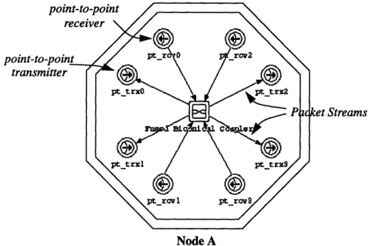
The Node level (See Figure 2-2) deals with the logical connection of components within a
connec-packets with no delay. Some Node level components exhibit properties, such as
propaga-tion delay and inserpropaga-tion loss, which can be modeled with a process designed at the Process
level. Other Node level components are used only as connections to links at the Network
point-to-transm
Streams
Node A
Figure 2-2: Node level model of a FBC node. Packets enter the node
through point to point receivers and exit the node through
point-to-point transmitters. The components in the node send packets to each
other through packet streams.
level. These components are called point-to-point transmitters and receivers.
The Process level (See Figure 2-3) allows for the design of Finite State Machine
pro-cesses found in many components in the Node level. This is where one finds the heart of
the AON Model Suite. These FSM based processes alter and delay the packets entering
the component in order to model the effects of the component.
Net-Figure 2-3: Process level model of a simple FSM containing one forced
state (init) and one unforced state (steady).
2.1.1 Packets
Packets are the primary means of communication in OPNET. Packets travel along links
and packet streams. The AON Model Suite uses packets to simulate the movement of light
in an AON. A packet either holds a single pulse or holds data representing a change in the
noise level.
2.1.2 Links
Links are connections between nodes at the Network level. Each link represents an optical
fiber or a bundle of optical fibers. Optical power travels along links in packets. A link is
defined by a number of procedures called the Transceiver Pipeline that, in the AON
Model Suite, modify traversing packets and calculate propagation delay in order to
simu-late light traveling through an optical fiber.
2.1.3 Nodes
Nodes are structures which are designed at the Node level and instantiated at the Network
level. Nodes are composed of components. While OPNET provides a wide variety of
com-ponent classes, the AON Model Suite only uses three -- the processor class, the
point-to-point transmitter class and the point-to-point-to-point-to-point receiver class. The point-to-point-to-point-to-point
transmit-ter class and point-to-point receiver class each supports only one type of component in the
AON Model Suite. The point-to-point transmitter class supports the point-to-point
trans-mitter component. The point-to-point receiver class supports the point-to-point receiver
component. The processor class, on the other hand, supports a large number of component
The point-to-point transmitter component sends packets along links at the Network level.
The point-to-point receiver component receives packets from links at the Network level.
The processor class based components manipulate packets according to a process
designed in the Process level.
2.1.4 Processes
In the AON Model Suite, processes are designed to model the properties of an optical
component. These processes are designed as Finite State Machines at the Process level,
and are made up of:
* Unforced states
* Forced states
* Transitions between states
Both types of states contain two sequential sections of C program code. When a process
enters an unforced state, it executes the C code in the first section of the state and then
exits. The unforced state resumes where it left off upon being woken up either by a packet
arrival or some other event, such as an event scheduled by the process itself, and executes
the C code in the second section of the state and progresses along a transition to the next
state. When a process enters aforced state, it executes the C code in both of the sequential
sections of the state and progresses along a transition to the next state. The transition
taken can depend upon the current state of the process.
2.2 Probing and Analysis
OPNET allows for the collection of statistics through the use of the Probe Editor. One can
specify probes in the Probe Editor in order to log statistics written out by components in
the simulation. Each processor class component in an OPNET simulation has an array of
2.3 A Simple AON Example
The following is a simple example to show how the AON Model Suite and OPNET work
together to simulate an All Optical Network. The example is an amplifier - fiber - filter
network (See Figure 2-4). The first event in the simulation is the transmission of a pulse
packet by the transmitter component. A pulse packet is represented by the symbol IJ.
This pulse (E)
travels over a packet stream to an EDF Amplifier component. The
amplifier modifies the packet by multiplying the signal by a complex transfer function in
the Fourier domain, and sends it on with a specified delay (n]).
Additionally, the
ampli-fier generates a noise packet (;).
A noise packet is represented by the symbol
.
These packets travel over a packet stream to the point-to-point transmitter component, the
device used to put packets on the optical fiber represented at the Network level by a
point-to-point link. The point-point-to-point transmitter component sends the pulse and noise packets
(
7)over
the
link.
These packets travel over the
link,
causing the AON Model Suite
defined Pipeline Stages to execute. These procedures simulate the fiber effects by altering
the pulse and noise packets. The link then forwards the modified packets (IZ)
to the
point-to-point receiver component. The point-to-point receiver component forwards these
packets (~
) to the fiber Fabry-Perot filter component, which modifies the packets by
passing them through a complex transfer function and sends them (
) with a
speci-fied delay to the receiver component. The receiver component collects statistics and
destroys the packets.
Figure 2-4: Simple AON Example to demonstrate how the AON Model Suite and
Chapter 3: Simulation Structure
In order to model an All Optical Network, one must have a model of the optical signals
traveling through the system, as well as models of each of the optical components. The
AON Model Suite is based on the propagation of pulses and noise through optical
compo-nents. As a pulse travels through the AON, it is passed from component to component and
manipulated appropriately depending upon the component type and parameters. Noise
also passes from component to component and is handled appropriately according to the
component type and parameters.
3.1 Simulation Global Variables
Several variables are maintained in the AON Model Suite that need to be accessed by
every component. These global variables describe the standard parameters of the pulse
and noise data, and are used by the components in manipulating the pulse and noise data.
The following global variables are maintained by the AON Model Suite:
*
Aonl_Nu describes the number of complex samples per pulse. 2 is the number of
complex samples per pulse. The number of samples per pulse is described this way
as a result of the use of the radix-2 Fast Fourier Transform algorithm throughout
the model suite.
*
Aonl_Len is the cached value of 2 , the number of complex samples per pulse.
*
AonI_Duration is the number of picoseconds sampled for each pulse. While pulses
may have a shorter duration than AonI_Duration, a longer duration results in
alias-ing of pulse data.
*
AonI_Low_Freq is the lowest noise frequency, in THz, tracked by the AON Model
·
Aonl_High_Freq is the highest noise frequency in THz tracked by the AON Model
Suite.
·
AonlN Segment is the number of noise frequency bands tracked by the AON Model
Suite. Increasing AonI N Segment increases the accuracy of the results due to
noise in the model suite.
·
AonI_Min_Power is the minimum significant power in the simulation. Pulse and noise
packets with power less than AonI_Min_Power are not transmitted.
·
Aonl_Min_Change is the minimum significant percentage change of noise power in a
noise band in the simulation. If the noise power changes by a smaller percentage
than AonI_Min_Change, the change will not be propagated.
·
AonI_Connectors is a flag indicating whether or not connectors are to be modeled in
the simulation. If AonI_Connectors is set, attenuation and reflection will occur at
connections between optical components.
·
AonI_Attenuation is the power attenuation factor of a connector. This variable is only
significant if Aonl_Connectors is set.
·
Aonl_Reflection is the power reflectance factor of a connector. This variable is only
significant if AonI_Connectors is set.
*
Aonl_Delay is the delay associated with a connector. This variable is only significant
if AonI_Connectors is set.
Table 3-1:Simulation Global Variables
Name
Type
Units
Description
AonI_Len
integer
N/A
Cached value of 2".
AonI_Duration
double
ps
The number of picoseconds
sam-pled for each pulse.
AonI_Low_Freq
double
THz
Lowest noise frequency tracked by
models.
AonI_High_Freq
double
THz
Highest noise frequency tracked
by models.
AonI N Segment
integer
N/A
Number of frequency bands into
which the noise spectrum is
divided.
AonI_Min_Power
double
W
Minimum power propagated
through the system.
AonI_Min_Change
double
N/A
Minimum percentage change of
noise power propagated through
the system.
AonI_Connectors
integer
N/A
Enables modeling of connectors
when not equal to 0.
AonI_Attenuation
double
dB
Attenuation factor of connectors.
Only valid when AonI_Connectors
is set.
AonI_Reflection
double
N/A
Reflectance of connectors. Only
valid when AonI_Connectors is
set.
AonIDelay
double
ps
Delay of a connector. This variable
is only significant if
AonI_Connectors is set.
AonI_Unco_Refl
double
N/A
Reflectance of unconnected port.
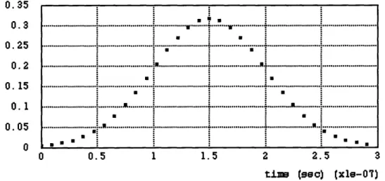
3.2 Pulse Structure
Pulses are the core of the AON Model Suite. Pulses are described by a data structure, the
most important field of which describes the shape. This field holds a pointer to an array of
envelope of the pulse. The complex envelope of the pulse describes the pulse shape in
terms of amplitude and phase (See Figure 3-1). One advantage to keeping track of the
complex envelope is the ability to transform the pulse using both linear and non-linear
models of pulse propagation. The choice of 2 samples is for efficiency in computing the
Fast Fourier Transform algorithm.
atts
Aon
.LI0. U.0.3
0.25
0.2
0. 15 0. 10.05
n ... . ... ...- ... ... E ... ...__ _ ... .i ... .i. . ... ... ... .. i *.. i * i i i i i "~~~~~~~~ , he~~~~~~~~~· 0 0.5 1 1.5 2 2.5 3ti
()
(xle-07)
Figure 3-1: The pulse shape is defined by 2 complex samples over a span of
AonI_Duration seconds. Here, Aonl_Nu = 5 and AonI_Duration = 300 ps.
The pulse data structure consists of seven fields:
* The source field holds the component identifier of the transmitter component that
gen-erated the pulse.
* The timestamp field holds the time at which the pulse was transmitted.
* Thefreq field holds the pulse carrier frequency.
·
The width field holds the FWHM (full width half-maximum) width of the pulse.
* The shape field holds an array of the complex samples of the pulse. There are 2
com-plex samples per pulse, where v is equal to AonI_Nu. The samples cover
AonI_Duration picoseconds.
Table 3-2:Pulse Structure
Name
Type
Units
Description
source
integer
N/A
Transmitter component identifier
timestamp
double
ps
Simulation time at pulse
transmis-sion
freq
double
THz
Frequency of the pulse carrier
id
integer
N/A
Pulse identifier
peak_power
double
W
Peak pulse power
width
double
ps
FWHM pulse width
shape
array
N/A
Array of complex samples
3.3 Noise Structure
Noise is tracked in a number of evenly distributed frequency bands, specified by
AonlN Segment, between the low frequency specified by AonI_Low_ Freq, and the high
frequency specified by Aonl_High_Freq. Noise is treated throughout the models as
inco-herent and of low power. These assumptions allow for ignoring non-linear effects with
respect to noise. Noise data travels through the system in packets. Each noise packet holds
·
freq_bin is
an integer from 0 to
(Aonl NSegment
- 1)
that indicates which frequency
band this structure describes. The center frequency of the noise band is
fbin
=
AonLowFreq+
Anl N Se0.5nt (Aon_I
High_F
req - Aonl_Low_Freq)
·
power is the optical power level of the noise in the band.
Noise travels through the simulation absolutely. That is, packets holding noise information
hold the current noise in a band. Noise in a noise band
Bf
at a port is equal to the power
value in the last noise packet describing that band:
Nsf = Nsf,
last
where Naf,
lastis the noise information in the last packet describing the noise band.
3.4 Ports and Port Structures
Each component in the AON Model Suite communicates with other components using
packets which travel over packet streams or links. Each packet stream is associated with a
source port and a destination port. Components send packets over packet streams by
send-ing them through ports (See Figure 3-2).
in
in
P
P2
When packets containing pulse or noise data arrive at a port they are transformed and
delayed by the component.
In a linear component with N ports, let
pout
(t)
P=
(t
out
in
(t))
be the port outputs and inputs.
The data coming in at a port can be divided into pulse and noise data, and each type is
dealt with differently. Because pulses travel through the simulator as complex amplitude
envelopes on a central carrier frequency, when a pulse is passed through a port it is
manip-ulated by a transformation matrix as follows:
Ppuse(t)
Spulseuse
(t
-D)
where
Spulse
=...
T N
1t N
... T NJ
where Ti
j
is a transformation of amplitude, and
D
is a delay. Depending upon the
compo-nent, the delay D can be either dependent upon the pulse frequency
(D
(f) ), or upon the
pulse frequency and component state (D (f,
state) ).
Noise, on the other hand, travels through the simulation as power. Thus, when noise is
passed through a port it is manipulated by a transformation matrix as follows:
out
in
IT,
N,
112pi
Pnos
e(t) = noiseoise (t - D)
where
Snois
e=
...
where
2
Tirj
is a transformation of power, and D is a delay. Again, depending upon the
component, the delay D can be either dependent upon the pulse frequency (D (f) ), or
upon the pulse frequency and component state (D (f, state) ).
The pulse and noise transformations in a linear system are described in general by the
lin-ear N x N S matrices
I,
1
(/)
...
HN I
f
*IH
()
IH (f)
N.
SL, pulse
...
..
.
and
SL,
noise
...H1
N
)
.
*
HN, N
H()
i,
...
IH
(f)Nij
where H (f) is a linear complex transfer function. The delay in a linear system, D (f),
imposed by the component is a function of signal or noise frequency.
The transformation in a non-linear system is described in general by the N x N matrices
SNL, pulse
SNL, noise
-HI,
1
(f' state) ...
HN,
1 (f, tate)
...
...
...
HI, N
(f,
state)
...
HN, N
V,
state)
IH (f,
state) 1, 1
2.. IH ( state)
... ... ...
I
IH
(f,
state),
1AJ
...IH (,
L -,I..' I
where state describes the state of the component. H (f, state) is a non-linear complex
and
* Port Pulse: This structure holds a list of pulses associated with the times they arrived.
This type of structure is necessary in non-linear models in order to maintain an
accurate representation of the state of the pulses coming into a port.
* Port Noise In: This structure holds an array of AonlN Segment noise power values.
This type of structure is necessary in order to maintain an accurate representation
of the state of the noise coming into a port.
·
Port Noise Out: This structure holds an array of AonI_NSegment noise power values
that represent the power leaving a port in addition to an array of Aonl_NSegment
noise power values that track the noise power values that the component has sent
through that port to the adjacent component. Essentially, when a change in the
noise power value in a specific frequency band
APchane
-INsf.current - Nf, last transmittedl
change f,current +
NSf,
last transmittedis less than AonI_MinChange
AP < AonI_MinChange
the change is deemed insignificant and is not sent. No changes are sent until the
current state is significantly different from the transmitted state. This structure,
while not strictly necessary, can improve the performance of the simulation
Figure 3-3: Flow diagram for linear component
3.5 Simulation Flow
Simulation flow is determined by the flow of pulses and noise through the AON
compo-nents. Pulses and noise travel in OPNET packets along OPNET packet streams and point
Initialize Module
Wait for event
Manipulate data
and send packet
Extract pulse or
noise data
Store data in port
data structure
Schedule interrupt for future time when
pulse or noise data will be manipulated
and forwarded to an output port
I
Figure 3-4: Flow diagram for non-linear component
non-linear the pulse or noise data is stored in a port structure, and an event is scheduled for
a time in the future when the pulse or noise data is to be passed on to the next component
(See Figure 3-4).
_ _
aket arriv
-emp
orschedule
-interrup
Airr va
Chapter 4: Component Models
The All Optical Network Model Suite includes a number of component models. There are
essentially six fundamental component types:
·
The transmitter components generate pulses. They are the only components that can
initiate a pulse travelling through the network.
·
The receiver component destroys pulses. It is the only component that causes pulse or
noise data to stop propagating in the network.
·
The probe component probes pulse and noise data.
·
The point-to-point transmitter and point-to-point receiver send and receive pulse and
noise data over links representing optical fiber.
·
Linear components receive pulse and noise data, transform it, and then send it on with
a delay to the appropriate component in the network.
·
Non-linear components receive pulse and noise data, remember it, and set an interrupt
for the time when they are supposed to transmit the pulse or noise data. At this
point, the non-linear effects have been determined, and the component transforms
the pulse or noise data appropriately.
These six component types are divided into three classes:
·
Essential: These components are essential to every simulation. The essential
compo-nents are the transmitter compocompo-nents, the probe component and the receiver
com-ponent.
* Fully Specified: These components have well defined complex transfer functions. The
* Partially Specified: These components are not well defined in terms of having an
accu-rate or complete complex transfer function. The partially specified components are
the star coupler, the ASE filter, the amplifier, the wavelength division multiplexer
and the wavelength router.
4.1 Transmitter
out
Fi]gure 4-1:
POin
Figure 4-1: AON Transmitter icon and port layout.
Incoming packets on port 0 are discarded.
Transmitters are the only AON component that can spontaneously generate optical
sig-nals. Transmitters generate a pulse with a given shape, and transmit that pulse to another
component in the AON. All transmitters share the following standard parameters:
·
source ID is the source identification number of the transmitter. Each pulse generated
holds the source identification number in its source field.
·
frequency is the pulse carrier frequency in THz.
·
peak power is the maximum intensity of the pulse.
·
to is a parameter related to the width of the pulse in picoseconds. For a gaussian pulse,
the Full Width at Half Maximum (FWHM) pulse width is equal to 1.763 to.
Table 4-1:Standard Transmitter Parameters
Name
Type
Default
Description
(Units)
source ID
integer
0 (N/A)
Identification number of
transmit-ter
frequency
double
192.0 (THz)
Carrier frequency of transmitted
pulse
peak power (Po)
double
0.1 (W)
Peak power of transmitted pulse
to (t
0)
double
100 (ps)
Parameter of pulse width
There are currently two classes
There is the gaussian transmitter
of transmitters, classified by the pulse shape generated.
class, and the hyperbolic-secant transmitter class.
The gaussian transmitter class generates gaussian (See Figure 4-2) and super-gaussian
(See Figure 4-3) pulse shapes defined by the following equation [Agr, 61]:
-1
+jCt ' 2mA (t) = /0e
2* m controls the degree of pulse sharpness. Higher values of m sharpen the pulse edges,
and cause the pulse to have a squarer shape. m is one for a gaussian pulse.
* C controls the linear chirp of the pulse. C is zero for an unchirped pulse.
rul. AAplltdu 0.3 0.25 0.2 0. 15 0. 1 0.05 ao
Figure 4-2: Gaussian pulse
amplitude (m =
to (p) lO1000O
1, t
o= 100ps, PO
=0.1 W).
rulue IAtlitUs 0.85 0.3 0.25 0.2 0. 15 0.1 0.05 0 tim (II (Cw 1000) I- ---- __ ._ __._
-L-
... .
... .
i
. .
0.25 . .5 0 0. 25 0. 5 0. TS I...
...
... ... ... ...0--
-
-
--
0I
:
7---
1
Ii·
0~ ~~~~~~~
02 05 0 I ITable 4-2:Additional Parameters for Gaussian Transmitter
Name
Type
Default
Description
(Units)
m (m)
integer
1 (N/A)
Degree of gaussian.
C (C)
double
0 (N/A)
Initial chirp of pulse.
The hyperbolic-secant transmitter class generates pulses with the hyperbolic-secant shape
(See Figure 4-4). This shape is important because it is the shape of a soliton. The
hyper-bolic-secant shape is defined by the following equation [Agr, 59]:
jCt
2A(t) =
4
u0
sech(
.t
2t
o
)
C controls the linear chirp of the pulse. C is zero for an unchirped pulse.
Pula p.it. l d 0.35 0.3 0.25 0.2 0. 15 0.1 0.05 0 0 0.25 0. 5 0.5 1 tim ps) (lOOO)
Figure 4-4: Hyperbolic-secant pulse amplitude (m = 1, t
o= 100 ps,
Po = 0.1 W).
Table 4-3:Additional Parameters for Hyperbolic Secant Transmitter
Name
Type
Description
(Units)
C (C)
double
0
(N/A)
Initial chirp of pulse.
I~~~~~~~
---
t---
~~
--
~~~
---Each transmitter class includes two transmitter models. For each class, there is a model
that transmits a single pulse, and a model that transmits a finite pulse stream. The single
pulse model for each class has the following additional attribute:
·
time is the transmission time of the leading edge of the single pulse.
Table 4-4:Additional Parameters for Single Pulse Transmitter
Name
Type
Default
Description
(Units)
time
double
0 (ps)
Transmission time of the leading
edge of the pulse.
The pulse stream model for each class has the following additional attributes which
describe a finite sequence machine:
·
start time is the time in picoseconds of the first transmission.
·
spacing is the amount of time in picoseconds between pulse transmissions.
·
repeat is a flag that when set indicates that the finite sequence should be repeated until
the end of the simulation.
*
initial state is the initial state of the finite sequence machine that generates the pulse
stream.
·
pn connections describes the connections in the machine.
·
state bits is the number of state bits in the machine.
Table 4-5:Additional Parameters for Single Pulse Transmitter
Name
Type
Default
Description
Table 4-5:Additional Parameters for Single Pulse Transmitter
Name
TypeDefalt
Description
(Units)
repeat
integer
0 (N/A)
Flag indicating whether or not to
repeat the finite sequence until the
end of the simulation.
initial state
integer
1 (N/A)
Initial state of the Finite Sequence
Machine.
pn connections
integer
3 (N/A)
Connections in the Finite
Sequence Machine.
state bits
integer
4 (N/A)
Number of state bits in the Finite
Sequence Machine.
A finite sequence machine generates a pseudo-random stream of bits. For example, the
four-bit finite sequence machine shown below (See Figure 4-5) generates a 2- 1 = 15
bit long stream before repeating.
Connection 3
f----
---- -_ASConnection 2
.
---
A\
Connection 1 on 0)lltnlt
bit 3
bit 2
bit 1
bit 0O
Figure 4-5: Four-bit Finite Sequence Machine: given a non-zero initial state, this
machine will generate allfour bit sequences for a total sequence length of
2 - 1 bits [Pet, 148]. This particular machine has an initial state equal to 1,
and a pn connections parameter equal to 3 (= 23c
3+ 22c
2+2 c
1+2 c
0)
because connections 0 and 1 are connected. In this machine, bit 3 in state n+1 is
equal to the exclusive or of the connected bits.
I , .
4.2 Optical Fiber
in
out
0
out
inFigure 4-6: AONFiber icon andport layout.
Optical fibers transmit pulses over distances in the AON Model Suite. Optical fibers
receive pulse and noise data at an input port, transform that data, and after a delay, send
the data out to an output port.
By default, the optical fiber model in the AON Model Suite models a single mode optical
fiber with a core area of approximately 65 ,gm
2, and a zero dispersion wavelength of 1.33
gm.
The optical fiber model takes into account both linear and non-linear optical phenomena.
The following effects are modeled:
* Attenuation is an effect that results in diminished pulse and noise power as a pulse or
noise travels along a fiber.
* propagation delay is the delay a pulse or noise experiences traveling along the fiber.
* dispersion is an effect resulting from the varying value of the index of refraction of the
fiber experienced by different wavelengths of light. This effect can alter a pulses
width and peak power.
* Self Phase Modulation (SPM) is a non-linear effect that results from a pulses intensity
com-·
Cross Phase Modulation (XPM) is a non-linear effect that results from the intensity of
a different pulse modulating the phase of the pulse. XPM results in the generation
of new spectral components to the pulse.
·
Stimulated Raman Scattering (SRS) is a non-linear effect that results in the
transfer-ence of power from a high frequency pulse to a low frequency pulse.
4.2.1 Fiber Parameters
Optical fibers in the AON Model Suite are defined by a number of parameters (See Table
4-6).
Table 4-6:Optical Fiber Parameters
Name
Type
Default
Description
(Units)
Length (L)
double
100 (kmn)
Length of optical fiber.
freql (fi
1
)
double
192.0 (THz) First reference frequency.
freq2 (f
2)
double
225.0 (THz)
Second reference frequency.
B1 at freql (
1 )
double
4875 (Ps
First term of dispersion
relation-km
ship at fi THz.
B 1 at freq2 (1,
2)
double
4872
s
First term of dispersion
relation-km
ship at f2THz.
B2 at freql (Pi2
j)double
2
Second term of dispersion
rela--20 (m)
tionship
at fi
.
B2 at freq2
(u
2
2)
double
2
Second term of dispersion
rela-0
(km)
tionship at f
2.
B3
(f3)
double
3
Third term of dispersion
relation-0
(E-
ship.
km
alpha (a)
double
0.2 (dB/km)
Attenuation per km.
A eff (Aeff)
double
65
(m
)
2Effective area of fiber core.
Table 4-6:Optical Fiber Parameters
Name
Type
Default
Description
(Units)
n2 (n
2)
double
3.2x10⁻¹⁶
The non-linear index coefficient.
2
cm
T Raman (TR)
double
0.005 (ps)
The Raman gain time coefficient.
granularity
double
1 (N/A)
Iterations of the spit step Fourier
method per length scale.
Grmax (gRmax)
double
1016( km
Maximum Raman gain.
Frmax (AfRmax )
double
12 (THz)
Width of linear section of Raman
gain spectrum.
The following parameters are derived from these parameters:
*
P
1 (carrier)or
P
1,f is the value of the first term of the dispersion relationship such
that:
P1,f-
P
1(fcarrier)
-=
1,
+
f
carrier
fi)
f2 4fi
* Vg (fcarrier)
is the group velocity of signal or noise power as a function of frequency.
1
4.2.2 Propagation Delay
Propagation delay of a pulse or of noise power is a function of the carrier frequency of the
pulse or the frequency of the noise band. The propagation delay as a function of frequency
is:
D (fcarrier)
=-
=L
1i
where
=
1
Vg V
4.2.3 Split-Step Fourier Method
The fiber model utilizes a method called the split step fourier method [Agr, 44] to
propa-gate pulses. The split step Fourier method is a method used to numerically approximates
the simultaneous effects of both the linear and non-linear effects of the fiber. The split step
Fourier method essentially approximates the simultaneous effects of the linear and
non-linear effects of the fiber by assuming that over a short distance, the non-linear and non-non-linear
effects can be assumed to act independently of each other [Agr, 44]. It is named the split
step Fourier method because it performs the linear effects in the Fourier domain, and the
non-linear effects in the time domain.
The length scales over which the fiber model propagates the pulse depend on the peak
power and width of the pulse. There is a length scale associated with dispersion, and a
length scale associated with the non-linear effects. Essentially, the fiber is chopped up into
sections according to these length scales. The dispersion length is given by [Agr, 52]:
LD=
1021
where To is the current FWHM width of the pulse. The non-linear length is given by [Agr,
52]:
1

![Figure 4-5: Four-bit Finite Sequence Machine: given a non-zero initial state, this machine will generate allfour bit sequences for a total sequence length of 2 - 1 bits [Pet, 148]](https://thumb-eu.123doks.com/thumbv2/123doknet/14443417.517336/43.918.125.747.570.769/figure-finite-sequence-machine-initial-generate-sequences-sequence.webp)