HAL Id: hal-01026188
https://hal.archives-ouvertes.fr/hal-01026188
Submitted on 21 Jul 2014HAL is a multi-disciplinary open access archive for the deposit and dissemination of sci-entific research documents, whether they are pub-lished or not. The documents may come from teaching and research institutions in France or abroad, or from public or private research centers.
L’archive ouverte pluridisciplinaire HAL, est destinée au dépôt et à la diffusion de documents scientifiques de niveau recherche, publiés ou non, émanant des établissements d’enseignement et de recherche français ou étrangers, des laboratoires publics ou privés.
Auditory Warnings for Electric Vehicles: Detectability
in Normal-Vision and Visually-Impaired Listeners
Etienne Parizet, Wolfgang Ellermeier, Ryan Robart
To cite this version:
Etienne Parizet, Wolfgang Ellermeier, Ryan Robart. Auditory Warnings for Electric Vehicles: De-tectability in Normal-Vision and Visually-Impaired Listeners. Applied Acoustics, Elsevier, 2014, 86, pp.50-58. �10.1016/j.apacoust.2014.05.006�. �hal-01026188�
Auditory Warnings for Electric Vehicles:
Detectability in Normal-Vision and Visually-Impaired Listeners
Etienne Parizet 1), Wolfgang Ellermeier2), Ryan Robart1) 1)
Laboratoire Vibrations Acoustique, INSA Lyon, Bâtiment St. Exupéry, 25 bis av. Jean Capelle, 69621 Villeurbanne, France; E-Mail: [email protected] 2)
Institut für Psychologie, Technische Universität Darmstadt, Alexanderstr. 10, 64283 Darmstadt, Germany; E-Mail: [email protected]
Abstract
Electrical vehicles operating at low speed are often too quiet to be detected by pedestrians in time. In order to study the efficiency of additional auditory warning signals they might be equipped with, a sample of 100 sighted and 53 blind listeners was exposed to a virtual road-crossing scenario in which they had to detect whether an approaching vehicle came from the right or left. Nine warning signals, designed to differ in particular sound features such as FM, AM or the number of harmonics were studied and compared with the recording of an unfitted electrical vehicle (EV) and a conventional diesel car.
The responses measured in the scenario in which cars approached at irregular intervals over two 20-min periods showed no reaction-time differences between blind and sighted participants, and a significant advantage when listening under dry weather conditions as opposed to recordings mixed with the sound of rain. Most importantly, however, regardless of listening conditions and the population studied (sighted or blind), the additional warning signals differed greatly in efficiency. Some signals facilitated detection of the EV as much as making it as noticeable as a control diesel car of significantly higher sound pressure level. Other signals were largely ineffective compared with the unfitted EV. Analysis of the signal characteristics suggested a relatively low number of harmonics, absence of frequency modulation, and irregular amplitude modulation to be the most salient features facilitating timely detection.
Key words: electric vehicle, auditory warning, alert sound, visually impaired, blind, pedestrian safety, reaction time
1. Introduction
At low speed, electric vehicles produce very little noise, as compared to gasoline or diesel engine cars. The noise level difference between an electric vehicle and one with an internal combustion engine (ICE) can be as large as 6 dB(A) at 10 km/h [1]. This difference becomes smaller at higher speeds. Above approximately 40 km/h, both types of cars are equally loud, because tire noise becomes the most important noise source.
In a city, due to ambient traffic noise, this lower sound level makes it more difficult for pedestrians – and much more dramatically for visually impaired ones - to detect an approaching electric vehicle. This was demonstrated by Garay-Vega et al. in a laboratory experiment [2]. Fourty-eight visually-impaired participants were presented with binaural recordings of conventional or electric vehicles approaching at low speeds (6 mph), in two kinds of background noise, differing in level (31 or 50 dB(A)). They had to detect the approaching car and made their response by pressing a computer key. Results indicated a higher number of missed detections for the electrically driven cars. Also, subjects detected ICE vehicles sooner than the EVs: the difference amounting to as much as 1.5 seconds. These results were confirmed by other laboratory studiess (e.g., [3, 4]) and by an in-situ experiment [5]: In this experiment, twelve visually impaired subjects had to detect an approaching car, driving on a very smooth road surface at a maximum speed of 30 km/h. At 10 km/h, ICE vehicles were detected at a safe distance (more than 10 m away). In contrast, the electric vehicle was detected only a few meters from the pedestrian. This might be dangerous for a pedestrian intending to cross a road. Indeed, a statistical survey [6] reports a significantly higher incidence of pedestrian or bicyclist crashes due to electric vehicles, though the low number of electric vehicles sold at the time this study was conducted makes the comparison a little difficult. In order to prevent this increased risk, manufacturers use, or plan to use, additional warning sounds, emitted by a loudspeaker attached to the front bumper or the wheel arch. Some specifications for these warning sounds already exist. As an example, the National Highway Traffic Safety Administration recommends values for the frequency bandwidth and sound level of such signals [7] and a similar regulation is currently being prepared by the European authorities. This last project defines acceptable warning sounds in a surprisingly vague manner: they should sound “similar to the sound of a
vehicle of the same category equipped with an internal combustion engine and the sound level may not exceed the sound level of a similar internal combustion engine vehicle” ([8], Annex IX,
part A, points 4.a to 4.c). Such a regulation would, of course, run counter to efforts to reduce traffic noise annoyance via the introduction of electric vehicles. Thus, there is a need for studies investigating the specification of efficient but low-level warning sounds.
While many papers about alarm sounds in work environments have been published (airplane cockpits, intensive care units or machinery rooms; see [9] for a review), only few studies have focused on warning sounds for low-noise vehicles. Yamauchi et al. used three warning sounds (engine noise, car horn and band-pass noise) in a laboratory study involving German and Japanese listeners [10]. The audibility of each sound was measured in different background noises. Results indicated a strong influence of the kind of warning sound, depending on the background noise. The difference reached up to 10 dB between the band-pass noise (which was the most easily detected sound) and the car horn. No cross-cultural difference in detectability emerged. Wall Emerson et al. [11] conducted an in-situ experiment for which five artificial sounds were synthesized and played back by a loudspeaker mounted to an electric vehicle.
Fifteen blind participants were seated at the side of the roadway and were asked to indicate when they detected the arriving car (at a speed below 20 km/h). Several trajectories were investigated (the car was moving on a straight line, or was making a right turn, etc.). Differences in the effectiveness of the five warning sounds in communicating these maneuvers were observed; unfortunately, the report fails to provide information about the levels of the warning sounds or other replicable acoustical specifications. The authors advocate that efficient warning signals should (a) have maximum energy around 500 Hz and (b) be amplitude modulated. Misdariis et al. used 10 sounds, which could be represented in a two-dimensional timbre space [12]. The first dimension was related to temporal modulation and the second one to spectral flatness (distinguishing a random noise from a tonal sound). The amplitude of the signals was modified so as to simulate an approaching source at 20 km/h. Six participants had to detect each sound in a background noise. Again, there were strong differences in the detectability of the sounds: the shortest reaction time (RT) was obtained for a siren sound (4 s) and the longest RT (11 s) for a modulated electric hum. Furthermore, there was evidence for differential learning effects.
Clearly, additional research on efficient warning sounds for electric vehicles is needed, particularly since the few studies on the topic have (a) only employed a limited number of warning sounds, (b) often did not vary them systematically, and (c) had very small samples of listeners, especially visually impaired ones to validate the efficiency of the signals. The present study aspired to fill these gaps by (1) designing warning signals by varying timbre parameters that have proved to be promising in previous research, (2) presenting these alerting signals in realistic roadside scenarios in which cars may approach from either side and in different weather conditions, (3) rendering these dynamic auditory scenarios with some degree of spatial auralization, and (4) evaluating the detectability of the vehicle-plus-warning sounds using both normal-vision participants and a relatively large sample of visually impaired listeners recruited by collaborating laboratories in several European countries.
As to the first goal of optimizing the sound characteristics for better detectability, the present study focuses on two sound features: (1) the frequency bandwidth of the warning sounds and (2) temporal modulation. While the NHTSA requirements [7] recommend minimum sound levels in eight third-octave frequency bands between 315 and 5000 Hz, one might consider it more efficient to concentrate the energy in a much smaller frequency region. This way, given a limited overall level, the warning sound is more likely to be heard in the presence of background noise. Furthermore, it is generally assumed that temporal modulation can help the listener to segregate the warning sound from the ambient noise. More specifically, research on auditory alarms [13, 14] has shown that increasing the rate at which components of a warning sound are presented also raises its perceived urgency. The effect of these timbre parameters will be investigated in the laboratory by measuring their effect on the detection performance of both normal-vision and visually impaired listeners.
2. Method
The main part of the experiment consisted of presenting an auditory road-crossing scenario to participants and to ask them to determine the direction from which a car approached in a background of traffic noise. In the following, the auralized situation and the warning stimuli used will be described in detail.
2.1 Stimuli and Design.
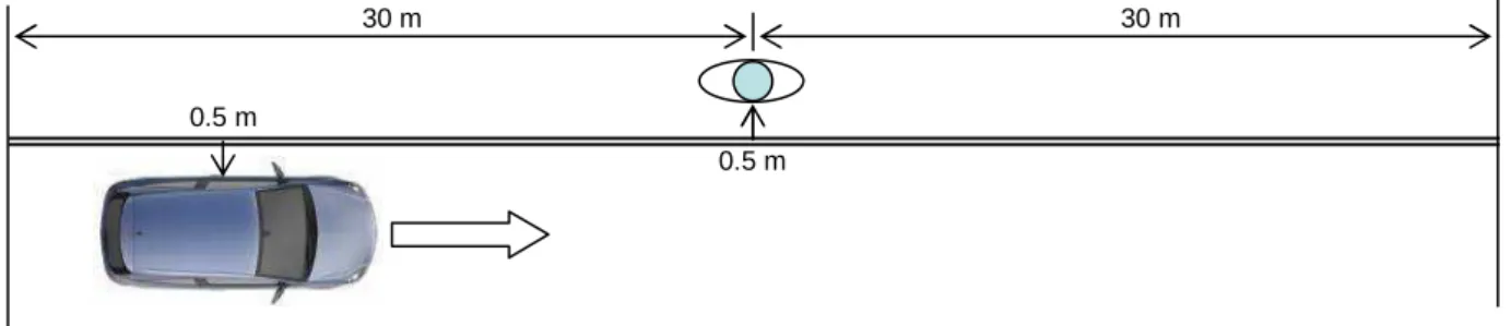
The simulated situation (depicted in Fig. 1) was one of a pedestrian standing on the sidewalk, close to the carriageway and facing it, about to cross the road. A car is passing perpendicularly in front of him or her, at 20 km/h, the smallest distance between the car and the pedestrian being 1 m (see figure 1).
Figure 1 Graphical depiction of the ‘waiting-to-cross’ scenario. The artificial-head
position is indicated on top. As indicated in the sketch, recordings were made at 1 m distance from a 60-m trajectory of the car with a constant speed of 20 km/h.
Two cars were recorded in this situation, using a dummy-head (Head Acoustics HMS II) at the location of the pedestrian. One of these cars was an electric vehicle (Renault Fluence) and the other one a similar car equipped with a diesel engine. Recordings were made from a distance of 30 m ahead of the dummy-head to the same distance past it, so that the duration of the signals was 10.6 s. The recording device (Brüel & Kjaer Pulse front end) registered the signals with a sampling frequency of 44.1 kHz and 16 bits resolution.
The warning signals to be added to the electrical vehicle sound were combinations of pure tones. Specifically, the influence of two timbre parameters was investigated: the number of sinusoidal components used and the presence of temporal modulation.
The bandwidth of the sounds was limited between 300 and 1500 Hz. The lowest frequency was selected because of technical limitations of the loudspeakers to be used on the future prototype. The small size of these loudspeakers limits their radiation efficiency to frequencies above 300 Hz. The upper limit was selected for two reasons. First of all, the hearing threshold below 1500 Hz is not greatly affected by age [15]. Secondly, one goal of the project is to combine a good detectability and a low overall level of warning sounds. Focusing the energy in a limited frequency band should allow the signal to be above the detection threshold in that band.
The warning sounds were synthesized according to a three-factor design varying (a) the number of sinusoidal components, (b) the amount of frequency modulation, and (c) the amount of amplitude modulation. All factors had three levels, which are detailed below.
- Number of components (factor 2 in the following). All stimuli were made of a set of harmonic frequencies, with the lowest component fixed at 300 Hz. At level 1, three frequencies separated by 300 Hz (300, 600 and 900 Hz) were used. At level 2, six harmonics separated by 150 Hz, and at level 3, nine harmonics each 150 Hz apart were generated, so that the frequency range was 300 to 1500 Hz. All harmonics had the same initial level.
0.5 m
0.5 m
- Frequency modulation (factor 1 in the following). At level 1, all components had fixed frequencies. At level 2, the frequency of the two higher components was sinusoidally modulated (∆f = 5%, fmod = 5 Hz for one component and 4 Hz for the other one, to introduce an asynchrony). At level 3, the same held for the two highest components, and a saw-tooth modulation – thus emphasizing the rising portion of the FM glide - was applied to the remaining components.
- Amplitude modulation (factor 3). At the level 1, no amplitude modulation was applied. At level 2, the signal amplitude was sinusoidally modulated (fmod = 8 Hz, Amod = 0.8). At level 3, the amplitude of the higher components was modulated in the same way as for level 2. The two lowest components, however, were modulated in a more complex way. The modulation frequency varied linearly between a low value (e.g. 0.8 Hz) and a high one (e.g. 16 Hz) in approximately 2 s and then suddenly came back to the lowest value. These parameters were different for the two components, which created large variations in the signal. This level will be denoted as "random" amplitude modulation in the following.
Rather than presenting all 3x3x3=27 combinations of the factor levels, in order, only a subset of the full factorial was used in what is called a fractional factorial design, this technique having proven to be useful to save listening time and gain statistical power in perceptual studies [16]. Table 1 shows the combination of factors and levels used in the plan. Consequently, nine stimuli were synthesized. They were equalized so that their A-weighted, energy-equivalent levels were equal. Stimulus Factor 1: Frequency Modulation Factor 2: Number of Harmonics Factor 3: Amplitude Modulation s1 none [1] 3 [1] none [1] s2 none [1] 6 [2] 8 Hz [2] s3 none [1] 9 [3] random [3] s4 sinusoidal [2] 3 [1] 8 Hz [2] s5 sinusoidal [2] 6 [2] random [3] s6 sinusoidal [2] 9 [3] none [1] s7 sawtooth [3] 3 [1] random [3] s8 sawtooth [3] 6 [2] none [1] s9 sawtooth [3] 9 [3] 8 Hz [2]
Table 1 : Warning signals and sound features used in the experiment (the levels of the three factors are indicated in brackets).
These warning sound stimuli were further processed (by one of the project partners: LMS International) in order to represent a moving omni-directional source, passing by at 20 km/h in front of the pedestrian. This computation included a reflecting road surface (according to
the ISO 10844 standard [17]). Head related transfer functions (from the CIPIC database1) were taken into account, so that the output of the computation was a binaural signal.
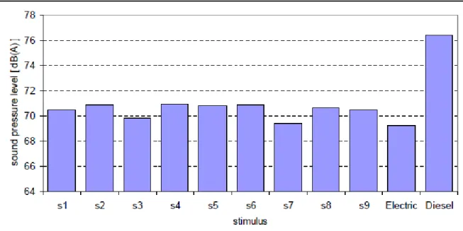
This signal was added to the recording of the electric vehicle. The mixing factor was selected by a trial and error process so that the warning signals were audible but not too loud. This mixing factor was set to be the same for all nine stimuli and resulted in an average signal-to-noise ratio of approximately -6 dB over the course of the signal. Thus, nine "EV plus warning sound" stimuli were obtained. The original electric vehicle recording and the one of the diesel car were added to the set of sounds, resulting in a total of 11 binaural stimuli. The sound pressure level of all 11 stimuli was computed, using the A-weighting and the fast time constant. Figure 2 represents the peak level measured for each stimulus, defined as the maximum of the peak levels of the two sound channels (i.e. the two ears of the dummy head).
Figure 2. Peak level (A-weighted SPL) of the vehicle sounds with (s1 - s9) and without
added warning signals (the two rightmost bars).
It can be seen that the maximum level of the electric vehicle is 7 dB(A) below the one of the diesel car, which is in accordance with the literature. This difference is greater than the one reported in [1], in which the conventional car was equipped with a gasoline engine, which tends to be quieter than a diesel. As can be seen in Figure 2, warning sounds amplify the level of the electric vehicle by 2 dB(A) or less. Though the A-weighted levels of the warning sounds were equalized before the moving-source simulation, this computation created slight disparities, due to the different frequency bandwidths of the sounds. Maximum loudness values (computed according to DIN 45631) varied accordingly, but exhibited very little variation, amounting to 24
1
sones for the EV alone, and ranging between 26 and 28 sones for the EV sound combined with the different warning signals.
2.2 Background noise
Two kinds of background noise were used. The first one was composed of different recordings, made using the same kind of dummy head. The intention was to simulate a background traffic noise far away from the listener (approximately 100 m) so that no confusion could occur between vehicles contributing to this continuous traffic and the approaching car to be detected. As the dummy heads were placed close to the traffic lanes during the recordings, the directional components of the noise were eliminated by mixing the two channels, thus obtaining a diotic signal. The samples were concatenated in order to obtain a rather stationary 2-min sequence which was looped continuously during the experiment. The intention was to simulate a background traffic noise far away from the listener (approximately 100 meters) so that no confusion could be made between vehicles contributing to this continuous traffic and the approaching car to be detected.
For the second background noise, the sound of rain was added to the same traffic noise. This was done because visually impaired people often relate that rain significantly increases their difficulty in understanding their sound environment in the street.
In the following, these two simulated road scenarios will be referred to as "wet" and "dry", respectively. Both were presented at a level of 69 dB(A). This level could fluctuate in a 3-dB range (when computed with a slow time constant).
2.3 Apparatus
The listening tests were conducted in double-walled (or at some sites single-walled) sound-attenuating chambers and controlled by a computer program written in Delphi 7.0 (Borland). The acoustical stimuli were stored on the hard disc and D/A-converted at 44.1 kHz and with 16 bit resolution via an external sound card (e.g. INSA: Echo Gina 24/96; TU Darmstadt: RME Multiface II). Subsequently they were passed through a headphone amplifier and delivered binaurally to high-quality headphones (e.g. INSA: Stax Lambda Pro; TU Darmstadt: Beyerdynamic DT 990). Presentation levels were verified using either an artificial head (Cortex Electronics MK1) or an ear simulator (Brüel & Kjaer Type 4152 6-cm3 coupler).
2.4 Procedure
The participants listened to the background noise, played continuously. At randomly selected times, one of the vehicle sounds was added to the background noise. The car could arrive from the right of the listener (i.e. as recorded on the track) or from the left (which was accomplished by swapping the two channels of the sound file). The road-crossing scenario was explained to the participants and they were told that their task was to detect the approaching car as soon as possible by deciding which direction it came from (left or right). In order not to confuse the vehicles to be detected with the background, participants were told that the target vehicles would appear to get much closer than the ambient traffic noise which sounded like a good distance away. Responses were made by pressing one of two keys on a standard keyboard:
the space bar in case the participant thought the car arrived from the left and the Enter key (on the right side of the numeric pad) in the other case. The inter-stimulus interval was randomly chosen between 1 and 20 s. Each stimulus appeared 8 times (4 times from each side of the listener), resulting in an overall number of 88 presentations and an approximate duration of the experiment of 45 minutes. In order to prevent the subject from getting too tired, the session was divided into two blocks of 44 sounds each. Between the two blocks, the subject was given some rest. Before the experiment started, several examples of the stimuli were presented to the participants and a short training session took place, during which five stimuli (randomly selected from the entire set) were used.
The data were written to a log file that recorded : the stimulus number, its starting time, the objective direction of arrival, the listener’s response time in ms measured from the onset of the vehicle sound, and the arrival direction as reported by the listener.
2.5 Participants
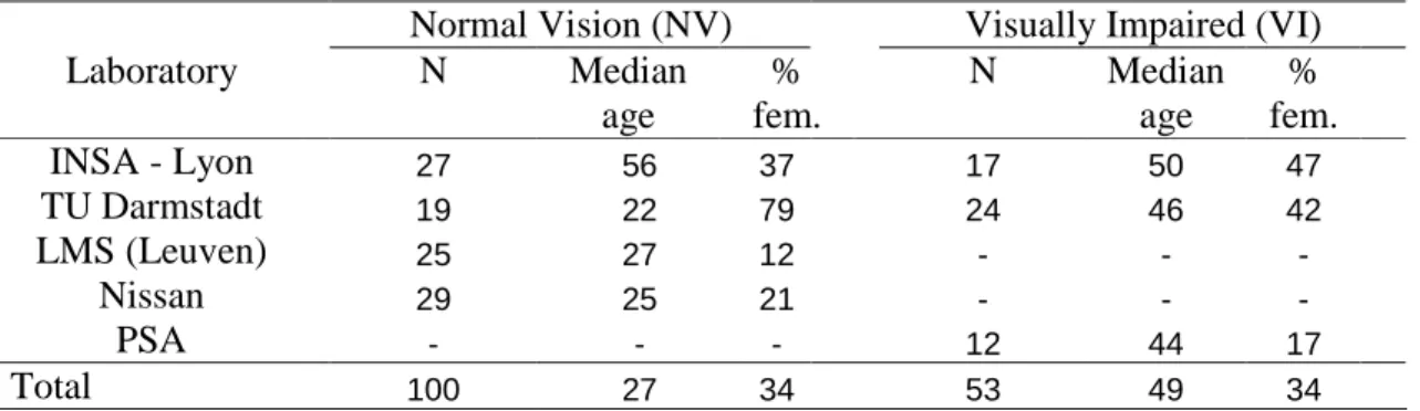
In all, 162 listeners volunteered to participate in the study. Nine of them were excluded on the basis of a high number of erroneous responses (for exclusion criteria: see results section), leaving us with a sample of 153 listeners (median age 38 years; range 20-72), to be further analyzed. 54 of them (i.e. 35%) were female, 100 of them had normal or corrected-to-normal vision (NV) and 53 were visually impaired (VI). All the VI participants were blind, and nearly all were visually impaired from birth or early childhood. Most sighted and VI participants reported normal hearing. However, occasional reports of mild, and often frequency-specific hearing loss were encountered among participants over the age of 60, none of whom felt participation in the present suprathreshold task was affected.
The participants were recruited by several project partners, i.e. in France, Germany, Belgium, and the U.K., from their local subject pool or by contacting organizations for the blind, and either just volunteered their time, or received a small monetary compensation, and in some cases course credit for participation. Their demographic characteristics are listed – separately for each study site and population - in Table 2.
Normal Vision (NV) Visually Impaired (VI) Laboratory N Median age % fem. N Median age % fem. INSA - Lyon 27 56 37 17 50 47 TU Darmstadt 19 22 79 24 46 42 LMS (Leuven) 25 27 12 - - - Nissan 29 25 21 - - - PSA - - - 12 44 17 Total 100 27 34 53 49 34
3. Results
3.1 Descriptive Statistics
Data were excluded from further analysis, if a given participant missed more than 20% of the stimuli, reacted after the vehicle had passed (RT > 5.4 s) or missed all presentations of a particular stimulus. Nine participants met one or more of these criteria, thus leaving 153 complete data sets to be analyzed.
In these data sets, errors (with respect to the direction of approach) occurred in a mere 3.45% of all trials. Therefore, subsequently, reaction times were analyzed based on all trials, whether correct or, in very few cases, incorrect, reasoning that the latter, too, imply successful detection of the vehicle (or warning) sound.
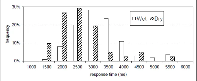
Figure 3 shows the distribution of all individual subjects’ mean response times, separately depicted for those listening in the dry (ND=44) and the wet (NW=109) background noise conditions. It is evident that participants differ considerably in their average RT, some detecting the targets as early as 1.3 s after their first appearance, others responding only when the vehicle has almost passed, i.e. after some 5 s. That corresponds to distances between 22.4 and 0.9 m from the observer positioned at the virtual roadside (see Figure 1).
Figure 3. Distributions of individual subjects’ mean overall reaction times, for recordings with
‘dry’ (N=44, hatched bars) and ‘wet’ (N=109, white bars) road conditions.
Even though based on means of 88 raw observations per data point, both distributions are somewhat skewed to the right, and show mean durations and inter-subject variability quite typical for choice reaction time: MD=2.317 s (SDD=0.877) and MW=2.957 s (SDW=0.775).
The direction from which the recorded vehicle was approaching did not exert a systematic influence on RT; paired t-tests showed left/right differences to be insignificant both in the dry, t(43)=0.002; p>.05, and wet, t(108)=1.7; p>.05, simulated weather conditions. Therefore, in subsequent analyses, RTs to vehicles approaching from the right or from the left were collapsed, yielding 8 rather than 4 repetitions per sound and participant.
3.2 Influence of the site of data collection
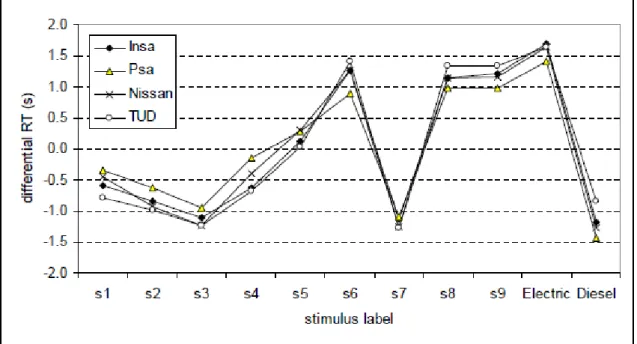
An important control variable to be inspected is the site at which data were collected, particularly since site is often confounded with the type of condition (e.g. dry vs. wet background) or population (sighted vs. VI) studied (see Table 2). It turned out that the site at which data were collected did have a significant influence, as determined by a single-factor, between-subjects analysis of variance (ANOVA), even when restricting the analysis to the wet background noise condition, F(3,105)=13.96; p<0.001 (There was no significant difference between laboratories for the dry background noise conditions). Particularly, RTs collected at two of the sites (PSA, Nissan) were some 0.8 to 1 s longer on average. That may be attributed to differences in headphones, sound insulation, and potential calibration errors, and is not entirely accounted for. As a remedy, RTs referenced to the overall mean of a given participant were inspected; these turned out to be quite similar when comparing the different warning sounds. Figure 4 shows such an analysis comparing the results of the four different laboratories as a function of the sound condition studied. It is evident that the RT patterns are remarkably similar despite the different offsets in overall RT. For the remainder of the analysis to be presented, the raw, unreferenced RTs were used.
Figure 4. Detectability of the sounds as measured in four different laboratories with the
simulated ‘wet’ background. The data have been normalized in that differences in RT referenced to each subject’s overall mean are plotted.
3.3 Blind vs. Sighted Participants
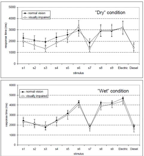
Figure 5 shows mean RTs for blind vs. sighted participants, both with the wet (bottom) and the dry background noise conditions (top). It appears that the overall mean RTs of the two
populations are quite close, and that the patterns of responses to the different sound stimuli are quite similar, even when comparing across the two road conditions (dry and wet).
To assess the statistical significance of these effects, a three-factor, mixed analysis of variance (ANOVA) was conducted on the average individual (unreferenced) RTs per condition, with sound (11 levels) constituting a within-subjects factor, and population (blind vs. sighted) as well as background (wet vs. dry) constituting between-subjects factors. Since means (across at least 8 repetitions), not unprocessed reaction times constituted the input for this analysis, a parametric approach was deemed appropriate. The ANOVA yielded a non-significant main effect of the population, F(1,149)=1.26; p=.263, and thus confirmed that the effect of visual impairment did not have a significant influence on RT. Even though the overall RT of the visually impaired participants was – despite their higher age - almost 250 ms faster on average (MVI=2.616; MNV=2.859), that difference was not statistically significant.
Figure 5. Mean reaction time to the different signals in blind (open circles) vs. sighted
participants (diamonds). The top panel shows reactions to signals embedded in a background noise simulating a dry road (NVI=19; NNV=25); the bottom panel shows the results for a ‘wet’ noise background (NVI=32; NNV=77) including the sound of heavily pouring rain.
There was, however, a significant (sound x population x background) three-way interaction, F(10,1490)=6.04, p<.001, indicating that the effect of the sounds differed for blind and sighted participants as a function of the background noise condition used. That is evident when comparing the top and bottom panels of Figure 5: Only in the dry background noise (top) do the RT patterns of blind and sighted participants seem to deviate from each other, suggesting that while the general pattern of responses to the warning sounds is quite similar, the blind participants’ responses are less uniform and thus differentiate slightly better between the different types of signals. The overall two-way interactions, by contrast, between the population studied and either sound, F(10,1460)=1.51, p=.13, or background, F(1,146)=0.049, p=.82, were not statistically significant.
3.4 Traffic noise conditions
Figure 6 affords a better comparison between the dry and wet (rainy) road noise conditions by re-arranging the data already presented in Figure 5. It is evident that the dry road condition facilitates earlier detection, particularly of the less salient warning signals, and of the pure electrical vehicle sound. That is confirmed by a highly significant main effect of the background condition, F(1,151)=19.77, p<.001, and further by a significant sound x background interaction, F(10, 1510)=34.20, p<.001, in the overall ANOVA specified in the previous section.
Figure 6. Mean reaction times of all (sighted and VI) participants to the warning signals in the
3.5 Differences between warning sounds
Figure 6 is also suited to compare the differences in detectability of the different warning sounds, the main effect of sound being the most significant of all considered in the ANOVA,
F(10,1490)=398.52, p<.001. It is evident that the differences in RT to the vehicle sounds are
considerable, exceeding 2 s for some comparisons, with RT to a given sound nevertheless being measurable with great precision.
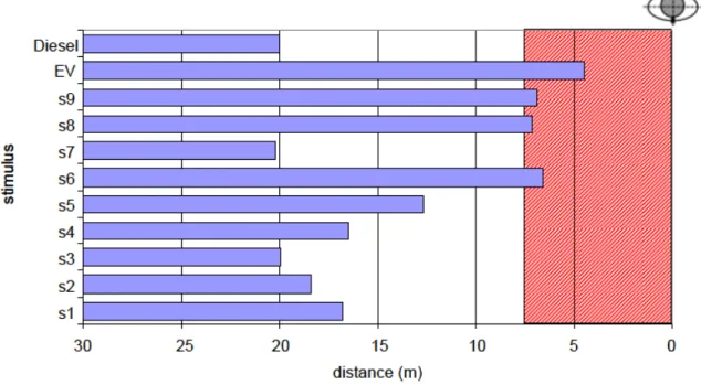
Figure 7 shows the same outcome when the reaction time in seconds is converted to the distance in meters in the virtual scenario at which the observer detects the vehicle. Remember, that the recorded vehicle was moving at a constant speed of 20 km/h, i.e. 5.5 m/s. It is evident, that on average, and with the more difficult (‘wet’) background noise condition, some vehicles – most notably the electric vehicle not supplied with an additional warning – are detected at ‘unsafe’ distances of less than 7.5 m. This distance represents the stopping distance at 20 km/h. It takes into account the reaction time of the driver and the time needed by the braking system to stop the car [5, 19]. Furthermore, the discrepancy in the estimated distances at which diesel and electrical vehicle are detected (here: some 16 m) is remarkably similar to what other investigators have observed in situ [5], thus lending some credibility to the present ‘virtual’ scenario.
Figure 7. Distance in meters at which the vehicles were detected in the virtual roadside scenario
(including rain). Measured reaction-times (Fig. 6) were converted to the distance in m (see Fig. 1) at which the observer indicated – via key press - to be able to tell the direction of approach.
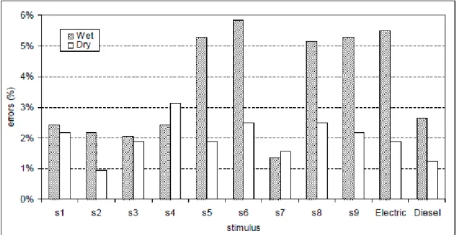
A post-hoc analysis of the differences between the recordings with added warning sounds suggests that, due to the large sample size, nearly all of them are distinguishable in terms of their effects on RT (see Figures 5-7). Most notably, sounds 3 and 7 appear to be the most salient, resulting in significantly faster RT (p<.001) than all other warning signals, making performance equally effective as detecting the approach of a noisy diesel vehicle of higher SPL. Interestingly, the same pattern of results was apparent in the (directional) errors made, meaning that responses did not exhibit a speed-accuracy tradeoff. Rather, those warning sounds leading to fast RTs also tended to produce fewer errors. This can be seen in figure 8, which represents the rates of directional errors for each stimulus, separately for the two background noise conditions.
Figure 8. Percentages of directional errors broken down by stimulus, as measured in the two
background noise conditions.
As for mean reaction times, there were no significant differences in directional errors when comparing sighted with visually-impaired subjects. Figure 8 shows that for some stimuli (namely, the electric vehicle alone and the warning sounds s5, s6, s8 and s9) these errors depended strongly on the background noise. On the other hand, other warning sounds produced very few errors, whatever the background noise condition (e.g., s1, s3 and s7).
Both of the warning sounds affording the fastest RTs and best directional discrimination contain (random) amplitude modulation (see Table 1), but differ in the presence of FM (none for sound No. 3) and the number of harmonics (nine for sound No. 3; three for sound No. 7). Therefore, a closer inspection of the sound features as specified by the experimental design is in order.
3.6 Statistical analysis of the effects of sound features
To evaluate the contribution of the various sound features to overall detectability, the sounds were analyzed according to the experimental design. Since the three levels of each of the features FM, number of harmonics, and AM were not presented in all factorial (3x3x3=27) combinations, but rather in a ‘fractional’ (33-1) design of only 9 combinations (see Table 1), a specific ‘fractional’ factorial ANOVA [16, 18] analyzing the three factors with respect to the levels at which they were presented was performed. The ANOVA applicable to the present design (investigating one third of the full factorial) is not suited to analyze interactions. Nevertheless, main effects (of the sound features) may be explored.
Figure 9 Effects of the sound features making up the warning signals. Frequency modulation
(F1), the number of harmonics (F2), and the presence of amplitude modulation (F3) were varied at three levels each (see text and Table 1).
The 3 (factor) X 3 (level) fractional ANOVA was performed on the mean individual reaction times of all participants (blind or sighted) and provided evidence for significant main effects for all three factors: Frequency modulation [F(2,974)=173, p<.001], number of harmonics [F(2,974)=137.7, p<.001], and amplitude modulation [F(2,974)=159.1, p<.001], the effects sizes being quite similar for all three factors. Figure 9 illustrates the effects of the three factors, i.e. the manipulated sound features, as a function of their respective level for that subset of data collected with the wet-road noise background. The outcome for the dry background – both descriptively, and in terms of the statistical analysis - is essentially the same. It is evident that amplitude modulation (open triangles in Figure 9) has a positive effect on RT, meaning that higher levels on the amplitude modulation variable (sinusoidal or random AM) tend to decrease RT, whereas the other two variables (FM: filled squares; Number of harmonics: filled circles in
Figure 9) produce the shortest RT at their lowest levels (i.e. with FM absent and just 3 harmonics).
4. Discussion
The present experimental study investigated the benefit of additional auditory warning signals superimposed on the sound of relatively quiet electrical vehicles. By pooling data from several laboratories, it managed to accumulate a considerably larger number of both blind (N=53) and normal-vision control participants (N=100) than earlier work had (e.g. [10, 11, 12]), thus resulting in greater statistical power to address the effects of (a) the intended population of listeners (visually impaired or not), (b) the listening situation (e.g. the aggravating circumstances having to detect the sound of an approaching car against a background of rain) and, most importantly, (c) variations of the acoustical parameters characterizing the additional warning signal.
As to the first issue, it is interesting to note that most studies of visually impaired listeners did not include a normal-vision control group, thus rendering a comparison with the research literature difficult. In the present study, the blind participants did not react significantly faster on average, which agrees well with results recently reported in a study of electric and ICE vehicle sounds without additional warning components [4]. If anything, the presence of additional warning sounds facilitated the blind participants’ responses slightly more than it did the normal-vision listeners’ performance (see the top panel of Figure 5), albeit only under ideal listening conditions, i.e. without interference from the sound of rain. The general pattern of benefitting from certain timbre variations in the warnings (see below), however, was the same for both groups of participants, thus encouraging the design of a universal warning signal serving both populations.
As to the acoustical background, it appears that the efficient stimuli (diesel engine, EVs supplemented with salient warnings) did not suffer from the addition of the sound of rain, while for the less efficient warnings, RT was prolonged by as much as 1 s (as is evident in Figure 6 and from the statistical interaction effect between vehicle sound and background). That suggests that studying different auditory listening conditions may in fact sharpen the distinction between different warning signals. Similar effects had been observed in earlier studies using different ambient noise conditions, though based on a much smaller number of vehicle sounds [2] or warnings [10].
Clearly, while the present study made an effort to render a relatively authentic auditory scenario with a realistic traffic-noise background, with binaurally recorded target vehicles approaching from either direction, and with simulated adverse weather conditions, there are obvious limitations. While, for example, the approach of the target vehicle was properly auralized, recordings of background or weather conditions were originally diotic and simply superimposed on the former, thus making it possible to detect the vehicle (and warning) based on changes in interaural rather than timbre cues. That, of course, might facilitate detection based on a favourable interaural configuration, but it does not invalidate comparisons between the different sounds studied which were all equally affected by this potential bias. Future research, however,
may attempt to improve rendering the spatial properties of not just the target signal by using appropriate binaural technology.
The most important goal of the present study was to identify those timbre parameters that make a warning efficient by reducing response times. To that effect, three factors were varied in the composition of signals, namely (1) the number of harmonics, (2) the presence and type of FM, and (3) the presence and type of AM in the warning sound. Analysis of the fractional factorial design used suggests that RTs are shortest when a small number of harmonics is used, when FM is absent, and AM is prominent and rather complex. Two warning sounds (No. 3 and 7, see Figures 5-7), both of which contained irregular AM, fared best in the empirical tests, and resulted in equal performance as detecting the much noisier diesel car. Curiously these sounds were also the ones having the lowest sound pressure levels (see Figure 2). The ideal sound, however, would have been one with three harmonics, no FM, and maximal AM, having minimal levels on the first two factors and the maximum level on the last one ([1,1,3] in the notation of Table 1). Though that sound was never presented to participants due to the sparse, fractional experimental design employed, the analysis suggests that it might have yielded performance just as good or better than with the most effective warnings actually evaluated. Thus, the present study shows that it is possible to design additional, synthetic warning sounds which do not, or only marginally increase overall level with respect to the unfitted electrical vehicle, and remain well below the sound levels generated by internal combustion engines. These warning sounds vary considerably in efficiency, depending on the adjustment of critical timbre parameters. In line with studies of warning sounds at the workplace (see [9]) these appear to be optimal, when the energy is focused on a small spectral region, and when there is appreciable temporal amplitude modulation. By optimally setting these features, reaction-times may be shortened by some 2 s, or more than 50% (see Figures 5 and 7). It might be interesting to explore, whether the present data can be accounted for by an auditory model [20] predicting simple RT to vehicle sounds from the masked thresholds of the approaching vehicles in a background of traffic noise.
Further studies will have to determine, whether the information transmitted by these warning sounds goes beyond discriminating the direction of approach (as investigated in the present study), and may be used to infer speed or the travel path with respect to the listener. Furthermore, it might be interesting to study to what extent the additional warning sounds in isolation, or when emitted by several vehicles, contribute to the overall annoyance of future, electric-vehicle traffic noise.
5. Acknowledgements
This research was funded by the European Union eVADER project (electric Vehicle Alert for Detection and Emergency Response; http://evader-project.eu, grant agreement No. 285095). A major portion of the work was conducted within the CeLyA ("Centre Lyonnais d'Acoustique", ANR-10-LABX-60) research network.
The authors would like to thank their collaborators in the eVADER project, namely Perceval Pondrom and Josef Schlittenlacher at Technische Universität Darmstadt (Germany), K. Janssens and F. Biancardi at LMS International (Belgium), J.C. Chamard from PSA Peugeot-Citroën (France), and D. Quinn as well as P. Speed-Andrews at Nissan (U.K.). They all contributed to the implementation and data collection of this study. The authors would like to further thank all
student research assistants involved and are particularly grateful to the blind listeners who volunteered their expertise for the experiments, showed great enthousiasm, and made many helpful suggestions. Preliminary results of this study were reported at the AIA-DAGA Conference in Merano (Italy), February 2013 and at the International Congress on Acoustics (ICA) in Montréal (Canada), June 2013.
References
[1] Japan Automotive Standards Internationalization Center (JASIC). A study on approach warning systems for hybrid vehicle in motor mode. Informal document n° GRB-49-10, 49th GRB, February 2009, available at
http://www.unece.org/trans/main/wp29/wp29wgs/wp29grb/grbinf49.html
[2] L. Garay-Vega, A. Hastings, J. Pollard, M. Zuschlag, M. Stearns, Quieter cars and the safety of blind pedestrians: phase I, DOT HS 811 304, National Highway Traffic Safety Administration (NHTSA), Washington, DC, USA (2010).
[3] J. Grosse, R. Weber, S. Van de Par, Comparison of detection threshold measurements and modelling for approaching electric cars and conventional cars presented in traffic and pink noise, Proc. ICA 2013 (Montréal, 2013).
[4] E. Altinsoy, The detectability of conventional, hybrid and electric vehicles sounds by sighted, visually impaired and blind pedestrians; Proc. Internoise (Innsbruck, 2013). [5] K. Glaeser, T. Marx, E. Schmidt, Sound detection of electric vehicles by blind or visually
impaired persons, Proc. Internoise (New York, 2012).
[6] J. Wu, R. Austin, C. Chen, Incidence rates of pedestrian and bicyclist crashes by hybrid electric passenger vehicles : an update, DOT HS 811 526, National Highway Traffic Safety Administration (NHTSA), Washington, DC, USA (2011).
[7] NHTSA, Minimum sound requirements for hybrid and electric vehicles. National Highway Traffic Safety Administration, n° NHTSA-2011-0148 (2011).
[8] European Commission, Proposal for a regulation of the European Parliament and of the Council of the sound level of motor vehicle. COM(2011) 856.
[9] A. Guillaume, Intelligent auditory alarms, in T. Hermann, A. Hunt, J.G. Neuhoff (eds.), The sonification handbook, Logos (Berlin, 2011), pp. 493 – 508.
[10] K. Yamauchi, D. Menzel, H. Fastl, M. Takada, K. Nagahata, S. Iwamiya, Cross-cultural study on feasible sound levels of possible warning sounds for quiet vehicles, Proc. InterNoise 2011 (Osaka, 2011).
[11] R. Wall Emerson, D. Kim, K. Naghshineh, J. Pliskow, K. Myers, Detection of quiet vehicles by blind pedestrians. J. of Transp. Eng. 139 (2013) 50-56.
[12] N. Misdariis, A. Gruson, P. Susini, Detectability study of warning signals in urban background noises : a first step for designing the sound of electric vehicles, Proc. ICA 2013 (Montréal, 2013).
[13] R. Patterson, Auditory warning sounds in the work environment, Phil. Trans. R. Soc. London, B327, 485-492 (1990).
[14] E. Hellier, J. Edworthy, I. Dennis, Improving auditory warning design : quantifying and predicting the effects of different warning parameters on perceived urgency, Human Factors 35 (1993) 693-706.
[15] International Organization for Standardization. Acoustics –Statistical distribution of hearing thresholds as a function of age. ISO-7029 (Geneva, 2000).
[16] V. Koehl, E. Parizet, Influence of strutural variability upon sound perception : usefulness of fractional factorial designs, Applied Acoustics 67 (2006) 249-270.
[17] International Organization for Standardization. Acoustics –Specification of test tracks for measuring noise emitted by road vehicles and their tyres. ISO-10844 (Geneva, 2011). [18] G. Box, S. Hunter, W. Hunter, Statistics for experimenters : design, innovation and
discovery, second ed., Wiley Interscience (2005).
[19] S. Kerber, The importance of vehicle exterior noise levels in urban traffic for pedestrian - vehicle interaction, ATZ Worldwide 108 (2006), 19-21.
[20] S. Kerber, H. Fastl, Prediction of perceptibility of vehicle exterior noise in background noise, Proceedings DAGA 2008, Dresden (Germany).