Towards Incorporating Within-Field Variation into Spatial Agronomic Decision Processes

(1)

HAL Id: tel-02548498

https://hal.archives-ouvertes.fr/tel-02548498

Submitted on 7 May 2020

HAL is a multi-disciplinary open access

archive for the deposit and dissemination of sci-entific research documents, whether they are pub-lished or not. The documents may come from teaching and research institutions in France or abroad, or from public or private research centers.

L’archive ouverte pluridisciplinaire HAL, est destinée au dépôt et à la diffusion de documents scientifiques de niveau recherche, publiés ou non, émanant des établissements d’enseignement et de recherche français ou étrangers, des laboratoires publics ou privés.

Towards Incorporating Within-Field Variation into

Spatial Agronomic Decision Processes

James Taylor

To cite this version:

James Taylor. Towards Incorporating Within-Field Variation into Spatial Agronomic Decision Pro-cesses. Sciences and technics of agriculture. Université de Montpellier, 2019. �tel-02548498�

(2)

MEMOIRE D’HABILITATION A DIRIGER DES RECHERCHES

T

OWARDS INCORPORATING WITHIN

-

FIELD VARIATION INTO

SPATIAL AGRONOMIC DECISION PROCESSES

James A. TAYLOR

(3)

Please reference as

Taylor, J.A. 2019. Towards incorporating within-field variation into spatial agronomic decision processes. Mémoire d’HDR, The University of Montpellier.

The defence of the thesis took place at SupAgro Montpellier on the 7th_{of June, 2019. The jury}

members were

Professor Phillip Vismara (Chair) – SupAgro Montpellier

Dr Gilbert Grenier – Bordeaux Sciences Agro (External Examiner) Dr Aurelie Metay _ SupAgro Montpellier (Internal Examiner) Professor Bruno Tisseyre – SupAgro Montpellierµ

Professor Jose Antonio Martinez Casasnovas - The University of Lleida, Spain. Dr Davide Cammarano – James Hutton Institute, Scotland, UK

Professor Christelle Gee – AgroSup Dijon was an external examiner but was unable to attend.

Please note, this has received a brief edit to correct grammatical and editorial errors. It differs slightly from the original submitted memoire, however, no additional sections have been added nor have any sections removed. References that are self-citations are indicated in bold within the text

This work is my own

James Taylor September, 2019

(4)

Acknowledgements

Since receiving my PhD degree in December 2014, I have spent the past 14 years as a Research Fellow or Senior Lecturer in various research institutions around the world. It has been challenging at time, and not always easy with a young family, however I have had a fantastic experience wherever I have been so far.

The number of people that have helped me on this research odyssey is enormous and I am sure that if I tried to list them all I would be sure to omit someone, somewhere. Therefore, to avoid this, I would just like to say at the outset an enormous thank you to everyone in Agriculture at The University of Sydney, Lincoln Ventures in Hamilton, NESPAL in Georgia, UMR LISAH and ITAP in Montpellier, CLEREL in NY and AFRD at The University of Newcastle. You have all aided in some way to shaping me and my academic journey to date.

There are a few people who have been a particular influence on my and whom I would like to single out and thank personally.

To Alex who set me on this path and to Brett who shaped my first post-doc in Sydney.

To Philippe who gave me such a wonderful welcome and opportunity to live and work in France. To Terry who took a chance to bring an Australian to upstate NY.

To Carlo and Rob who gave me such great support and confidence at Newcastle. To Jim and Clive for all their support and friendship in UK PA, and

To Bruno, for simply everything. Thank you. I could not have done half these things without your help. Finally, life is not all about work and the biggest influence and support that I have received has always come from home. So my final and biggest thanks is to Athanasia. You give me so much more than I could ever achieve on my own.

James Taylor 28/11/2018, Montpellier

(5)

List of Figures and Tables

Table 1.1 A summary of some key definitions of Precision Agriculture (and

site-specific crop management) proposed over the past 25 years. The selected references represent the general range of definitions provided and not all cited definitions are given here.

17

Figure 1.1 Graph of annual average dryland wheat yields from Australia and South

Africa (1990 - 2015). Data obtained from BFAP 2014 and ABCS 2013. The graph is reproduced from the www.grainsa.co.za website.

10

Figure 1.2 Examples of some early (1995-99) yield maps from Australia (reproduced

from McBratney et al. 2000). Maps a), b), d) and e) are grain yield, c) is grape yield. Yields are scaled (µ = 0) to present them on a common legend. Yields in the cereal systems tend to range from < 1 to > 5 t.ha-1_{; grape yield ranged from < 10 to > 30}

t.ha-1_.

11

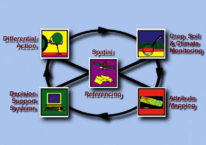
Figure 1.3 The Precision Agriculture wheel model showing the five main processes

for a site-specific crop management system (reproduced from Precision Agriculture

Laboratory, The University of Sydney,

https://sydney.edu.au/agriculture/pal/about/what_is_precision_agriculture.shtml).

13

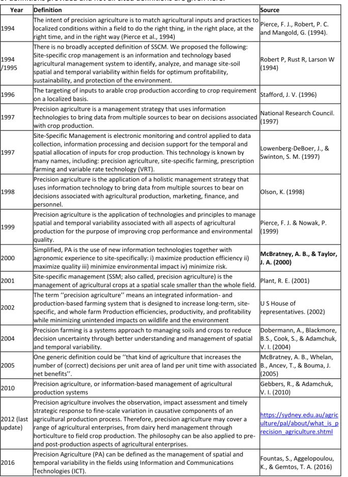
Figure 2.1 A time-series of yield maps from a field in North-western NSW, Australia.

The 1997 and 2006 maps show distinct management patterns amd the intervening years illustrate differing spatial patterns. Yield data are presented as standardised yield values. The variation in yield patterns associated with management but also with climate vs. soil effects in the field illustrate the difficulty that growers have in interpreting yield (and other production data) visually.

22

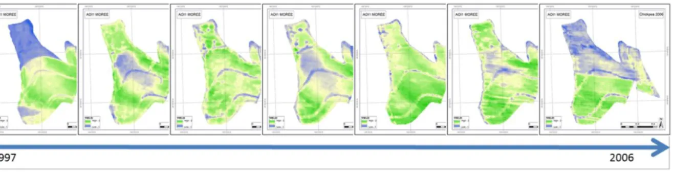
Figure 2.2 Adoption rates in the USA of key agri-technologies that facilitate

Precision Agriculture (site-specific crop management). Reproduced from Sonka and Cheng (2015). Satellite imagery has multiple applications but the dominant use is for assessing canopy development to inform nitrogen fertiliser applications.

24

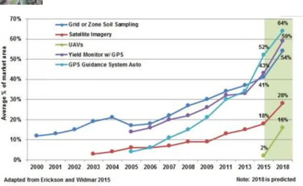
Figure 3.1 Schematic illustrating the preferred operational domains for academic

institutions and industry enterprises and likely funding support using the concept of Technology Readiness Levels. The disconnect and lack of funding at intermediate TRLs is clearly indicated and provides a barrier to successful innovation and technology translation.

28

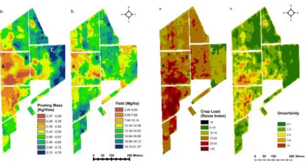
Figure 3.2: An example of mapping both a desired attribute (Crop Load or Fruit:Leaf

ratio) in vineyards and the potential uncertainty in the derived layer. The Crop Load map derives from a yield map and a calibrated canopy vigour map and contains potential errors associated with sensing, calibration and interpolation (adapted from Taylor et al. 2018b)

33

Figure 4.1 Selected examples of published variograms [(1) – (4)] and variogram

parameter tables (5). (1) Kiwifruit dry matter and fruit size variograms from NZ that were used to determine sampling grids for optimal map production (Taylor et al.,

2007b); (2) Average annual variograms for grain yield and grain protein in Australia,

illustrating similar variogram structures for the two variables (Whelan et al., 2009);

(8)

(3) Changes in variogram structures for pruning mass as the sampling size (number of vines) changed, which helped inform new sampling designs for vine size estimation (Taylor and Bates, 2012); (4) Standardised ‘average’ variograms of potato yield and tuber size parameters in both ware and seed systems that were used to identify management effects on spatial variance (Taylor et al., 2018a); and (5) variogram parameters and trend residuals for the determination of spatial structure in yield data sets from cereal, cotton and vineyard systems (Pringle et al., 2003).

Figure 4.2 Yield maps of four hypothetical fields of equal area and differing

characteristics in yield variation. Field (a): relatively large magnitude, relatively poor spatial structure; Field (b): relatively small magnitude, relatively moderate spatial structure; Field (c): relatively large magnitude, relatively moderate spatial structure; Field (d): relatively large magnitude, relatively strong spatial structure. It is hypothesised that the opportunity for SSCM will increase with Fields (a)–(d) with Field (d) having the greatest opportunity because its yield map displays both a large magnitude of variation and a strong spatial structure (from Pringle et al. 2003)

39

Figure 4.3 A 2014 grape yield map from a Concord (Vitis Labrusca cv Bailey) vineyard

in the Lake Erie Region of NY State. Boxes A and B show regions where yield relates to environmental variations (A) and where yield shows strong linear effects associated with management (B). The numbers on the graph are block identifiers (1 – 11) (from Taylor et al., 2018c)

41

Figure 4.4 Schematic illustrating the shift from a conventional uniform field

management strategy to a true site by site-specific management strategy by using zone (management unit) management as an intermediate. The required increase in data with the shifts are also indicated. (Image courtesy of the Precision Agriculture Laboratory, The University of Sydney).

42

Figure 4.5 A visual illustration of the protocol outlined in Taylor et al. (2007) to

transform raw irregular crop and environmental data into flat single layer maps and the fusion of these layers into a potential 2-management unit map (using k-means classification). The image was first published in CSA News, which is an industry magazine that supports research published within ASA, CSSA and SSSA journals.

44

Figure 4.6 A comparison of yield stability zones derived for two fields using

PCA-based image analysis of interpolated yield maps (Left images) and the same maps classified into yeidl stability classes using k-means classification. The top field is from North-west NSW Australia (and the same field used in Figs 2.1 and 4.5). The bottom field is from Northumberland in North-east England. The PCA-based method (left images) show clearer patterns with less fragmentation than the k-means approach. (Images reproduced from Blasch and Taylor, 2018)

45

Figure 4.7 A comparison of the application of a spatially constrained classification

(left) (Frogbrook and Oliver, 2007) and a novel segmentation (right) algorithm to canopy vigour data in a vineyard in Spain. For both approaches a 2, 4, 6 and 10 ‘class’ solution was found. For classification, this generates k classes, while the segmentation generates k (discrete) ‘zones’. The 4-class solution explains a similar level of variance as the 10-zone map but has three times as many discrete ‘zones’. (Image and details from Pedroso et al., 2010)

(9)

Figure 4.8 Left: An illustration of how management units (MU) could be used to

establish treatment ‘sub-plots’ to investigate input (nitrogen) response. No fertiliser, average (default) or double rates were applied in each MU. A yield monitor and a ProSpectra sensor were used on-combine to obtain yield and protein values for the treatments in each MU. MU 1 (red) had high pre-season soil N and additional fertiliser actually decreased yield. MUs 2 and 3 exhibited different responses, which were easily explained by agronomic practices. N response and optimum N differed between MUs (from Whelan et al., 2005).

49

Figure 4.9 Local maximum yield production potential map (left) based on yield data

collected from 2003-2015, and the corresponding multi-annual local production gap (right) (average % difference between the highest observed value and the annual values in each pixel). This has been computed on aggregated pixels but could be applied to MUs. (from Leroux et al. 2019)

50

Figure 4.10 Top - images showing grapes on a grape harvester discharge conveyor, a

harvesting operation, the load cells mounted on the side of the discharge conveyer and the display within the tractor cab. Bottom - Three validation plots to compare the calibrated yield sensor against different scales of measured mass; From left to right these were i) mid-season buckets for crop estimation (~30 kg), at-harvest trial plots (~’400 kg) and truck loads delivered to the crush (~20 ton). The at-harvest calibration is stable even for small masses. There is a midseason bias in sensor operation that needs recalibrating but the relationship remains strong and linear (images from Taylor et al., 2016).

51

Figure 4.11 Example of assessment of a prototype commercial on-combine grain

protein sensor (AccuHarvest, Zeltex Inc.). The sensor was supported by academic staff over three seasons and sampling performed to compare the on-combine protein sensor with a benchmark lab system at the grain silo. Calibration fits for each year (2003-05) are shown on the left and farm level maps of yield and protein to illustrate the spatial patterning of both variables (right) (from Whelan et al., 2009).

52

Figure 4.12 How effective co-design is predicted to accelerate technology adoption

by bringing forward adoption by “followers” and “laggards” thus boosting the adoption curve. This is achieved by 1) Co-design with end-users in the technology development phase to generate reasonable expectations and reduces the possibility of a new technology being overhyped; 2) Consideration of the socio-economic and technical barriers and appropriate extension service type mechanisms; 3) Twinning the technology with correct policy, regulation and service support to reduced time to ‘full’ market penetration – that is, peak adoption will be bought forward in time; and 4) Increasing penetration of the technology and generating higher rates of adoption by considering ‘laggard’ barriers which are likely to be underpinned by socio-economic rather than technical issues. (reproduced from Clark et al. 2018)

55

Figure 4.13 Conceptual model of barriers to and drivers of adoption of PA

technologies by end-users and interactions between drivers and barriers. The schematic was populated from a literature review on PA adoption and discussions with a variety of growers, industry service providers and academics (from Li et al.a.,

submitted)

(10)

Figure 4.14 A theoretical model of intention for PA adoption that links a need

technology fit (NTF) model with an adapted unified theory of acceptance and use of technology (AUTAUT) model. Multiple hypotheses (denoted Hx) were proposed to understand and model farmer behaviour. A blue arrow links the latent variable with the observational variables in a measurement model and black arrows indicate the hypotheses proposed in this study (from Li et al.b., submitted).

56

Figure 5.1 A conceptual illustration of how Precision Agriculture will intersect with

molecular diagnostic tools, computer science and social science domains to enable producers to make better decisions across all aspects of production, particularly in areas of crop health and quality.

(11)

1 - Introduction:

1.1 Background

The environment in which the majority of global crop production occurs is a variable environment1_.

Only in closed situations, e.g. glass/greenhouse and growth chamber conditions, is it possible to control edaphic and meteorological variation. These conditions, however, only account for a fraction of global production area, for example there were 720,000,000 ha of cereals grown globally in 20162

compared with 498,000 ha of total greenhouse production in 20173_{. Production variation occurs in}

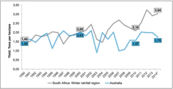
both time and in space. Dryland (rain-fed) systems are particular vulnerable to temporal variability, as production potential is strongly determined by the amount and timing of precipitation and any management to react to changing environmental conditions. The fluctuations in annual average wheat tonnage/ha from Australia and South Africa highlight this temporal variability (Fig. 1.1) at a national scale, but the same can be observed at enterprise, field and sub-field scales too. In Australia, where I started my research journey, national average dryland wheat yields can vary from < 1 t.ha-1_{to above}

2 t.ha-1_{, and this is when averaging climatic conditions across an entire continent! Regional differences}

can be more extreme.

Figure 1.1 Graph of annual average dryland wheat yields from Australia and South Africa (1990 - 2015).

Data obtained from BFAP 2014 and ABCS 2013. The graph is reproduced from the www.grainsa.co.za

website.

1_{Only plant production systems are considered in this document. Variability in animal production, both indoor} intensive and outdoor extensive systems is also important, and addressed in the domain of Precision Livestock Farming (PLF). While many of the variability concepts and technologies considered in the document have applications in PLF, they are only discussed in terms of cropping systems.

2_{Sourced from}_{https://data.worldbank.org/indicator/AG.LND.CREL.HA}_{(November 2018)}

3_{Sourced from International Greenhouse Vegetable Production – Statistics, 2018 Edition, Cuestra Roble} Consulting, www.cuestaroble.com/statistics.html

(12)

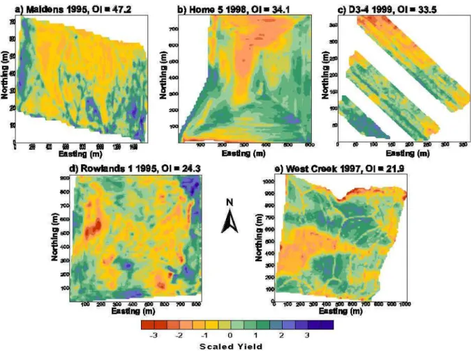
Spatially within fields, production can exhibit even greater variation within a season. Yield monitoring from the early-mid 1990s has consistently revealed large patterns in yield variance in cereal systems (Fig. 1.2 shows some different examples of this).

Figure 1.2 Examples of some early (1995-99) yield maps from Australia (reproduced from McBratney

et al., 2000). Maps a), b), d) and e) are grain yield, c) is grape yield. Yields are scaled (µ = 0) to present them on a common legend. Yields in the cereal systems tend to range from < 1 to > 5 t.ha-1_{; grape}

yield ranged from < 10 to > 30 t.ha-1_.

Producers are therefore confronted with temporal variance (predominantly in climate) interacting with spatial variance (predominantly soil and/or management effects) in their production systems. Until fairly recently, it has not been possible to correctly characterise the spatial variance in soil and crop properties, let alone the spatio-temporal variance in production, within a field (Fig. 1.2 for yield examples). It has always been possible to determine temporal variance at a whole field-scale. Field records are generally well kept by growers and suppliers for accounting purposes. Thus, it has been field or farm-level information, and some ‘best guess’ information on near and long-term climate conditions, that has historically driven crop decisions with the aim of optimising management to the ‘average’ of a field. The development of, and recent explosion in, sensing systems, which are linked to global navigational satellite systems (GNSS) (e.g. GPS), that measure and geo-located plant growth,

(13)

production attributes and soil properties has changed this situation. Growers and agronomists now have potential access to a wealth of high-resolution spatial data to help make management decisions. In the first instance, this should help to improve ‘average’ management, but the real opportunity lies in being able to make differential spatial and spatio-temporal management decisions at a sub-field level.

However, the opportunity to make more and better spatial decisions is also paired with the potential to make the wrong spatial management decision. Having access to more data does not directly translate to better (higher-resolution) decisions. There is a logical flow from data to information to decision that needs to be followed and adapted in the context of the end-user (growers/agronomists) and the target production system. In this context , the diversity in agricultural production, even just crop production, means a one-size fits all solution will rarely, if ever, be feasible. If the end-user cannot make a better decision, then the entire process (data collection, processing, data-fusion and interrogation) is redundant and worthless. This is a challenge that the precision agriculture community has always faced. Advances in sensing and communications mean that data exists (although it may still be incomplete or not exactly the right data needed). Methodologies to convert data and compress them into information layers are developed or developing rapidly. However, the leap to decisions is often still missing. If a decision exists, then the ability to enact the decision (an engineering problem) generally exists or can be quickly solved. The general process for PA implementation, which is a derivation of a process quality control cycle, is visualised in Fig. 1.3.

In situations where simple decision making is possible e.g. “Am I driving straight and at a fixed swath distance with an auto-steer tractor?”, then the uptake of technology has been shown to be fast and effective. Agronomy is unfortunately rarely ‘simple’; it is a biological process in a variable environment. There is a real challenge for agriculturists, engineers, computer scientists and the industry to make this work. Ideally, every time the circle in Fig. 1.3 is completed, an improvement in the decision and management process should be obtained. These are likely to be mostly incremental gains unless new disruptive technologies or methodologies are introduced that change the grower’s ability to either sense, analyse, decide or apply.

The general background discussion above has used dryland (non-irrigated) cereal (wheat) production primarily as a ‘classical’ agronomy example. However, spatio-temporal variation in all cropping systems has been reported or is expected because management and environment is never 100% constant. Irrigated systems tend to be more resilient to annual variations in weather, especially drier years, but are unable to cope with excess precipitation, for example. Perennial crops, often irrigated and intensively managed, are affected by production and environmental conditions in the current year

and the previous years. Therefore, how to determine the amount, the drivers and the decisions to

manage crop production is a universal question in arable, horticultural and viticultural systems. The term crop production in the introduction is deliberately ubiquitous, and slightly ambiguous in the previous statement. Site-specific crop management began with yield (quantity) management, because yield monitors were the first crop production sensing systems available. Crop quality is also important, and perhaps more so than yield in high quality production systems, and should also be considered in spatial decision-making.

(14)

Figure 1.3 The Precision Agriculture wheel model showing the five main processes for a site-specific

crop management system (reproduced from Precision Agriculture Laboratory, The University of Sydney, https://sydney.edu.au/agriculture/pal/about/what_is_precision_agriculture.shtml).

1.2 Outline of the Memoire

In this memoire I will present my journey and the knowledge that I have gained within the Precision Agriculture domain over the past two decades. The first section broadly introduces variation in cropping systems and serves as a very general introduction to the research domain.

Section 2 provides a more detailed overview of PA and develops some of the main issues and challenges that have been historically faced by PA practitioners. This includes clearly defining the domain and a recognition of the diversity and multi-disciplinary nature of PA. The role and importance of variability in production systems is then introduced along with the challenges in correctly and properly defining production variance. The final three parts of Section 2 turn the focus to how information, particularly multiple layers and multiple types of information, start to be translated into decisions. This shifts PA from a technical question on measuring and managing variation to a socio-technical innovation question on how technology is perceived and adopted and the potential disconnect between what scientists consider important and what commercial users want.

(15)

Section 3 further develops two key areas – the disconnect between academic research and commercial application (innovation) and the disconnect in the data that we have and what we want (in terms of data type and the quality). There is a deliberate focus on how PA technologies and methodologies are effectively translated into successful commercial services and what I have learnt about this from my various placements and from my attempts to define industry-facing protocols at various stages of my research career.

Section 4 provides an overview of how my research activities and publications that have (I hope) helped to address the issues raised in Sections 2 and 3. A focus is given to a large body of work that provides a descriptive reference base to observed spatial variation in yield and crop quality parameters in various annual and perennial systems. This is followed by the role and the evolution in zonage approaches over the past 2 decades and how these zones or management units have been used as a basis for more advantaged analysis to improve crop production knowledge and ultimately crop management decisions. The latter parts of Section 4 shift from natural, agronomic applications to more recent research that has started to interrogate and to build models to understand socio-technical aspects of PA. It develops ideas on how PA translation and adoption can be enhanced by better considering barriers and drivers of adoption.

The last section, Section 5, outlines my own vision for the evolution of Precision Agriculture over the next decade. It outlines how Precision Agriculture needs to develop so that producers have a more ‘personalised’ agricultural decision system. It highlights key areas of research that I would like to pursue in my future career, and how advances in digital technology will help to achieve this research and translation. There are some concluding remarks.

Throughout the memoire, I have deliberately avoided the incorporation of mathematical notation. I have preferred to keep the discussion more general and not too specific for a broader audience. The cited references contain more specific details for those wishing to understand the derivation of the geostatistical approaches and models discussed. By convention, I have indicated in bold the references that are self-citations within the document. These are all listed in the Bibliography. A more detailed publication list is appended with my full publication list. The publication list contains work that is not cited in the document, particularly research that I have performed in soil science, rather than in PA, and teaching and industry-oriented publications.

1.3 Personal Motivation

My journey into precision agriculture began within the domain of soil science, principally pedometrics and digital soil mapping (before the term was coined). Soil science always interested me through school, when soil erosion and the threat of land degradation was on the national conscious in Austraila in the late 1980s. When I went to university to study agriculture, I naturally gravitated towards a major in soil science. I have always been (and continue to be) fascinated in the way that soil forms in a landscape and the variation that is observed. I was also interested in the mathematical way that this variation was being described and mapped. My interest in how and why soil varies in the landscape ultimately led to an interest in how soil variation within a field impacts and creates spatial variation in crop production. And so, I entered the domain of precision agriculture, initially with an honours thesis

(16)

describing spatial and temporal variation in wheat fields, then a PhD thesis on Precision Viticulture and Digital Terroirs. This was followed by a series of post-doctoral positions in precision agriculture and digital soil mapping, which lead to a senior lectureship at Newcastle University and ultimately to Irstea and UMR ITAP. Throughout these endeavours, my research has always been strongly linked to industry needs and often I have been located on research stations and farms or working directly with growers and grower groups. It is a facet of Precision Agriculture that I love, bringing something new to the ancient art of agriculture while respecting the tradition and history behind productions systems. I hope that it continues.

(17)

2 - Context of the Theme of Research to Date

2.1 The philosophy of precision agriculture

Precision Agriculture (PA) is still a relatively new term in global agriculture, although with the recent development of Digital Agriculture it is no longer the ‘new kid on the block’. Precision Agriculture has its origins in grid soil surveying in the late 1980s in the USA (Pierce et al., 1994; Stafford, 1996). However its real birth came with civilian access to global navigation satellite systems (GNSS) and the development of on-combine and on-tractor sensing technologies. Linking the two generated an ability to map grain yield, a better appreciation of the inherent variation in yield (e.g. Fig. 1.2) and a desire to better manage this. In the 1990s, PA grew through a series of conferences and workshops and spawned its own specific academic journal in 2000 (Precision Agriculture Journal, Springer, New York, NY, USA). While the journal and many of the conferences continue as specialised PA forums, PA applications can now be found within more generic crop and agronomy forums, and it is now more common for PA articles to be found in ‘mainstream’ agriculture journals.

Definitions of PA are many and varied and reflect its diverse and diffuse origin. A legacy of its origin in soil sampling and mapping for crop nutrition is that in many definitions the ‘Agriculture’ in ‘Precision Agriculture’ tends to relate to cropping systems only. Suggestions that ‘Site-Specific Crop Management’ (SSCM) should be preferably used for PA applications in crop systems have been made (Robert et al., 1994; Plant, 2001). However, the term PA remains synonymous with cropping systems. Agriculture of course is much more than cropping systems. Animal-oriented studies however, tend to go by the term Precision Livestock Farming (PLF), rather than sit under the umbrella of PA. This is evident in Europe with both a biennial European Conference on Precision Livestock Farming (ECPLF) and a European Conference on Precision Agriculture (ECPA, which is strongly crop-oriented).

Table 1 gives some existing definitions for Precision Agriculture and their origin. Some are very specific while others are more general and inclusive. From my perspective, I tend to view PA in a more generic context and as a management philosophy rather than as a specific technological application. Precision Agriculture is about working out how to make better decisions, usually using emerging technologies. It is not based on any single or suite of technologies and innovations. It exists at the interface of innovation and agriculture, with the focus on improved resolution in spatial and temporal management. If it operates correctly, the PA of yesterday should be the ‘normal’ agriculture of tomorrow. The science and the community of Precision Agriculture should have ‘evolved’ into the next level of innovation and opportunity. Thus, it could now be considered that auto-steer tractors are no longer precision agriculture in many places, but part of good agricultural practice. Of course, GNSS-enabled equipment continues to be essential for many potential and developing PA applications.

(18)

Table 1.1 A summary of some key definitions of Precision Agriculture (and site-specific crop

management) proposed over the past 25 years. The selected references represent the general range of definitions provided and not all cited definitions are given here.

Year Definition Source

1994

The intent of precision agriculture is to match agricultural inputs and practices to localized conditions within a field to do the right thing, in the right place, at the right time, and in the right way (Pierce et al., 1994)

Pierce, F. J., Robert, P. C. and Mangold, G. (1994).

1994 /1995

There is no broadly accepted definition of SSCM. We proposed the following: Site-specific crop management is an information and technology based agricultural management system to identify, analyze, and manage site-soil spatial and temporal variability within fields for optimum profitability, sustainability, and protection of the environment.

Robert P, Rust R, Larson W (1994)

1996 The targeting of inputs to arable crop production according to crop requirement

on a localized basis. Stafford, J. V. (1996) 1997

Precision agriculture is a management strategy that uses information

technologies to bring data from multiple sources to bear on decisions associated with crop production.

National Research Council. (1997)

1997

Site-Specific Management is electronic monitoring and control applied to data collection, information processing and decision support for the temporal and spatial allocation of inputs for crop production. This technology is known by many names, including: precision agriculture, site-specific farming, prescription farming and variable rate technology (VRT).

Lowenberg-DeBoer, J., & Swinton, S. M. (1997)

1998

Precision agriculture is the application of a holistic management strategy that uses information technology to bring data from multiple sources to bear on decisions associated with agricultural production, marketing, finance, and personnel.

Olson, K. (1998)

1999

Precision agriculture is the application of technologies and principles to manage spatial and temporal variability associated with all aspects of agricultural production for the purpose of improving crop performance and environmental quality.

Pierce, F. J. & Nowak, P. (1999)

2000

Simplified, PA is the use of new information technologies together with agronomic experience to site-specifically: i) maximize production efficiency ii) maximize quality iii) minimize environmental impact iv) minimize risk.

McBratney, A. B., & Taylor, J. A. (2000)

2001 Site-specific management (SSM; also called, precision agriculture) is the

management of agricultural crops at a spatial scale smaller than the whole field. Plant, R. E. (2001)

2002

The term ‘‘precision agriculture’’ means an integrated information- and production-based farming system that is designed to increase long-term, site-specific, and whole farm Production efficiencies, productivity, and profitability while minimizing unintended impacts on wildlife and the environment

U S House of

representatives. (2002)

2004

Precision farming is a systems approach to managing soils and crops to reduce decision uncertainty through better understanding and management of spatial and temporal variability.

Dobermann, A., Blackmore, B.S., Cook, S., & Adamchuk, V. I. (2004)

2005

One generic definition could be ‘‘that kind of agriculture that increases the number of (correct) decisions per unit area of land per unit time with associated net benefits’’.

McBratney, A. B., Whelan, B., Ancev, T., & Bouma, J. (2005)

2010 Precision agriculture, or information-based management of agricultural production systems

Gebbers, R., & Adamchuk, V. I. (2010)

2012 (last update)

Precision agriculture involves the observation, impact assessment and timely strategic response to fine-scale variation in causative components of an agricultural production process. Therefore, precision agriculture may cover a range of agricultural enterprises, from dairy herd management through horticulture to field crop production. The philosophy can be also applied to pre- and post-production aspects of agricultural enterprises.

https://sydney.edu.au/agric ulture/pal/about/what_is_p recision_agriculture.shtml

2016

Precision Agriculture (PA) can be defined as the management of spatial and temporal variability in the fields using Information and Communications Technologies (ICT).

Fountas, S., Aggelopoulou, K., & Gemtos, T. A. (2016)

(19)

With this in mind, it is the definition of McBratney et al. (2005) that best defines PA for me.

“Precision Agriculture is that kind of agriculture that increases the number of (correct) decisions per unit area of land per unit time with associated net benefits.”

This definition does not specify system type (arable or perennial crops, animal, pastoral, etc…), nor does it link to specific technologies or methodologies. It emphasises that PA is about decisions. It is a philosophical statement that sets a goal for PA to make better decisions at finer spatial and/or temporal resolutions with the intent of making agriculture better. It is also (deliberately) ambiguous in how agriculture is made better i.e. it has ‘associated net benefits’. In an ideal application, these net benefits will be economic (production), environmental and social in nature, however it may be that only one or two are actually realised with any individual PA application. Collectively, a PA program should address all three aspects to ensure long term sustainability (economic, environmental and social) and enhanced food security. Typically the economic benefits are well understand and quantified (and easily derived in terms of monetary units), however the environmental and social benefits are poorly defined and quantified (Ancev et al., 2005).

Precision Agriculture has typically been advocated and employed in developed agricultural systems with higher levels of mechanisation. Applications into developing agricultural systems, including subsistence farming structures, are far fewer. However the philosophy of PA is as just applicable to small-scale and developing systems, even if the level of technological innovation in these systems is not as high. While mechanisation may be lower, management is often more (spatially) intense and can still be spatially varied, provided suitable tools for better decision-making are available. These of course need to be low-cost, user-friendly and effective, however there are globally increasing levels of disruptive technologies, notably smartphone and tablet technologies, which are providing a platform for PA applications in all types of agriculture systems (Lagos-Ortiz et al., 2018; Camacho and Arguello, 2018). The key, as alluded to previously, is of course to have the correct decision process for each type of system and for each location, i.e. a ubiquitous platform but a site-specific decision system.

2.2 PA - A multi-disciplinary domain

Achieving PA is no longer an agricultural science question. Precision Agriculture is about developing sensing systems to gather more or new data and information and decision systems to process and act on these systems. It is dependent on advances in many other disciplines to advance itself. At the core there will always be a need for good agricultural science but this operates around developments in sensing technologies (the domain of Electrical/Chemical engineers), data management and display (Computer Scientists), data analytics (Bioinformatricians and Statisticians) and PA machinery (Agricultural engineers). Precision Agriculture is a truly multi-disciplinary domain, especially when the social and economic components are added to the technical. With such multi- and inter-disciplinary needs, it is almost impossible for the complete PA skill set to be present in any single individual. Precision Agriculture must therefore be exist within collaborations and multi-disciplinary teams, within which diverse groups (or individuals) support and enable each other.

(20)

This provides an enormous challenge for the PA community. Agriculture is not always seen as a ‘sexy’ area to work in. Neither does it command the financial power of many other industries (e.g. defence, mining, financial, etc…) where data analytics and engineering skills are equally sort after. There is a challenge for the PA community to attract and to retain people capable of crossing over between engineering, data analytics and agricultural science. This is not to expect such people to be an expert in all areas, but rather to have a fundamental understanding of how the other areas impact innovations in their main speciality. Biological systems, and particularly intrusive systems like agricultural production systems, are not intuitive systems for applications of pure sciences. It is a highly variable and often changeable environment in which practical applications and trade-offs are needed. This is often difficult for people unfamiliar with agriculture to understand, however it is these people (engineers, computer scientists etc…) that are needed to make PA work.

Precision Agriculture works when all aspects are integrated. Figure 1.3 shows the ‘PA cycle’, which follows a typical quality control cycle operating under the general approach of Plan  Act  Check  Plan  Act  etc… In Fig. 1.3 this has been slightly expanded to consider Monitoring (Check), Attribute Mapping and Decision Support (Plan) and Differential Action (Act). The cycle is made possible by the ability to geo-reference all actions and analysis using Global Navigation Satellite Systems (GNSS), such as GPS (the USA Department of Defense’s Global Positioning System). Monitoring is performed by a variety of sensing systems that utilise a variety of chemical, physical and spectroscopic approaches and are mounted on a variety of different platforms (from terrestrial fixed or roving platforms to satellite platforms). The conception and development of these systems usually requires non-agricultural scientific and engineering expertise. Mapping, analytics and decision support development must always be done with the production system in mind. Information and decisions need to be tailored to the limitations of production. However, the expertise to create these analytical and decision systems lies in computer science and informatics domains, not in agricultural science. The knowledge to populate the systems does lie with agricultural scientists and agriculturists. Once a decision is made, technology, particularly variable rate technology, is needed to act on the decision. This requires the development of software controllers and variable-rate machinery, i.e. electronic, electrical and agricultural engineers teamed with computer scientists and software developers. This PA cycle, and any quality control cycle, is only effective at improving efficiencies if the cycle is completed and becomes a continuum where improvements are made with every rotation. From this perspective, there are no shortage of monitoring technologies available. The amount of data gathered is not-limiting, although there are still production variables that of interest that are not currently monitored. How raw data are processed into information, particularly single layer/variable maps, is generally well understood, although alternatives and advances continue. Likewise, controllers and hardware for variable rate applications and differential action are well developed and commercially available and quickly developed when a need is identified. The weak point in the cycle is the decision support step. Differential action will only be successful if the correct differential decision is given to the controllers. Decisions require information AND agricultural knowledge to be integrated and applied spatially.

Decisions in agriculture are reliant on the quality of data (and information) gathered, are affected by the economic and production goals of the system (farmer), are needed to be made in a spatially and temporally varying biological system and are dependent on previous and future management

(21)

decisions . In short, decisions are made in an imprecise systems with few situations where there is an absolute and correct decision. Optimising spatial decisions-making and demonstrating improved efficiencies is the biggest challenge to the further the development, acceptance and translation of PA.

2.3 The nature of variation in crop production.

Agricultural decisions are imprecise (not absolute) because the majority of agriculture exists within an open biological environment. When production interacts and reacts to variable environmental and biological conditions, production becomes temporally and spatially variable. From a PA context, the amount and nature of variation in a production system is a key determinant of the direction and opportunity for making decisions, determining the (absolute) quality of those decisions and imposing differential management (Pringle et al., 2003; Roudier et al., 2011).

In small-holder agriculture, qualitative PA is often practiced. Growers farm small areas that they interact with directly on a continuous basis and have a deep knowledge of the productivity across their (small) farm. This situation was the norm in developed agricultural economies before the mechanical and green revolutions of the 20th_{Century, and it still exists in many less developed agricultural}

economies (particularly parts of Asia, Latin America and Africa). Smallholder agriculture tends to respond to changes in productivity through manual interventions, but usually without quantitatively characterising the variation. For example, areas where seed germination is known to be lower may receive more hand-sown seed to promote a more even emergence. Input use efficiency has a quasi-optimisation process because of the knowledge of the grower in these situations and the general reliance on manual operations that can be adjusted based on existing knowledge.

The rise of mechanised agriculture and the green revolution led to farmers being able to farm larger areas, which included land they may have had no history with and limited knowledge of. The larger areas and use of machinery also decreased the time spent by the grower physically interacting with the land. In this new, larger production system, uniform (average) management of larger fields became the best economic model for crop production. Variation in yield and quality attributes was known to occur, but in the absence of historical knowledge and a lack of real-time information on exactly where and by how much production varied, the best solution became to farm to the average. Machinery was also geared towards large-scale average input applications. GNSS availability in the late 20th_{century changed the ability to locate information in fields, with some data traceable to within}

a few centimetres. This, coupled with development of crop sensors, meant that the location and amount of production variation and environmental variability could be recorded and analysed. Average, uniform management is no longer the most efficient model for modern crop production. However, recording this additional information comes at a cost, as does changing from a uniform to a spatially differential management system. The production efficiencies or other ‘associated net benefits’ must outweigh these additional costs for a producer to transition to differential management i.e. site-specific crop management may intuitively have a higher input use efficiency but it may not be more profitable than a ‘uniform’ management system and therefore not attractive to a farmer. There are several ways that the nature of the production variation affects the ability of a farmer to react to this variability and to transition to PA management;

(22)

1. If the magnitude of production variation is low, then there is potentially little to gain from variable management. A field that varies between 3 and 8 t.ha-1_{with an average of 6 t.ha}-1_for

a given crop will likely have more potential efficiency gains than a field that also averages 6 t.ha -1_{but with a range of 5.5 to 6.5 t.ha}-1_{. Applying an average input for a 6 t.ha}-1_{crop is closer to}

optimal in all locations in the second field than the first.

2. If the observed variation is random, then regardless of the magnitude, it is not possible to respond to the variation. In most cases, variation is not random, but there are strong differences in the amount of trend and the size of coherent spatial patches between fields. Fields with larger spatial patches tend to be more suitable for differential management and more compatible with current variable-rate technologies.

3. Is the cause of the variation obvious and manageable? If the cause of the variation is not identifiable then it cannot be managed. Similarly, in some cases the cause of the variability may be known, but cannot be corrected by the farmer through management operations.

4. To what degree is the observed production variability ‘independent’? This in itself has two facets- a) does the variable (e.g. yield) respond primarily to one level of input (e.g. N), or is it an interaction of multiple inputs (e.g. N x K x Irrigation), and b) does the variable have an effect on another aspect of crop production (e.g. if wheat yield is spatially managed does this impact spatial wheat protein (quality))?

Points 1 and 2 indicate how the (spatial) structure of variability can determine if progression into differential management is (likely) possible or not. Points 3 and 4 relate to the role that variation has in determining how decisions are made, and the implications of spatial decision making, if PA and differential management is to be implemented.

Points 4 also has implications for those building decision support systems as well as for these using them. Predictive models and crop simulation models are an increasingly important part of modern agriculture. Accurate and timely short and long-range predictions are invaluable for both managing and marketing agricultural production. Most of these models operate at large scales (regional, enterprise of field level). If they are to be spatialised or converted into spatial models, information on the expected variation is needed.

2.4 Spatial data fusion and decision systems in agriculture

High-resolution spatial data sets are relative new in agriculture and the way that the data and information are presented is still novel to many producers and industry actors. Interpreting maps of production attributes is not always intuitive (Taylor and Whelan, 2013). Individually, single biomass images, yield maps or soil maps are relatively easy for producers and agronomists to interpret and to superimpose their own knowledge onto. This is particularly true when there are clear management effects and/or environmental effects in the data/information. As more layers of data and information become available for a field, the ability to process the additional data/information diminishes. Figure 2.1 provides an illustration of this. It shows 7 different years of grain yield maps corresponding to different management decisions and to different climatic conditions. Each individual year is easily explained, however, when asked to simplify the maps and to integrate the multi-year data into a single map (e.g. a map of potential management units) the process becomes more difficult for the grower.

(23)

Which layers should be ignored? Which layers should be weighted as more important? This becomes more complicated if multiple years of biomass (canopy reflectance) imagery and soil maps are also added to the mix. It becomes even more complicated if some of the raw data are poorly presented or poorly mapped.

Figure 2.1 A time-series of yield maps from a field in North-western NSW, Australia. The 1997 and

2006 maps show distinct management patterns and the intervening years illustrate differing spatial patterns. Yield data are presented as standardised yield values. The variation in yield patterns associated with management but also with climate vs. soil effects in the field illustrate the difficulty that growers have in interpreting yield (and other production data) visually. (Data supplied by Mr M. Smith and images adapted from Blasch and Taylor, 2018)

If precision agriculture is about better decision making, then it is paramount that the way data are presented, the way that data are transformed into information layers and the way that data and information are fused into a decision process is done correctly. The more confusion that is generated at the initial stages, the harder it is to arrive at a good decision at the end. Approaches to filtering (e.g. Blackmore and Moore, 1999), mapping (e.g. Whelan et al., 1996) and integrating data (e.g. Lark and Stafford, 1997) have therefore been key areas of research from the inception of PA. Without these basic building blocks, making decisions and therefore PA adoption and translation is not possible. Filtering and mapping approaches continue to be updated (e.g. Sun et al., 2013, Leroux et al., 2018a), but the transformation of raw data into information layers is relatively well understood by academic and industry actors. How these data are then compressed, fused or simplified remains an issue for the industry. Methods, and well accepted approaches exist, however the on-going evolution in the amount and type of data available is constantly challenging the way that these data can be integrated and interpreted. Data fusion and the transfer of relevant information into decision systems remains a key area of development for PA. The more effective such methods are, the better the resulting decisions should be.

2.5 Adoption and translation in PA

Precision Agriculture is like any other advancement. Its movement from theory and development into application and translation follows the same laws/theory and pathways as other technological innovations (Koundouri et al., 2006). However, Precision Agriculture is about making better decisions,

(24)

it is not about a new method or a new technology (although in general these are the advances that are making higher spatial- and temporal-resolution decisions possible in agriculture). If the end-user cannot perceive a benefit in a new PA technology or methodology it will not be incorporated into management. Regardless of the quality of the technology/methodology, the benefit tends to come down to

a) an ability to understand and make a different decision and, b) an ability to quantify the benefit of the new decision.

New and emerging technologies in agriculture tend to fall into two categories, i) embedded knowledge or ii) information intensive. Embedded knowledge technologies have no (or very little) additional skills or training needed to gain value from the value ‘embedded’ in the technology. In contrast, information intensive technologies require the end-user (grower or agronomist) to gain additional skills or training to gain value from the technology (Miller et al., 2018).

The difference in adoption between embedded knowledge and information intensive technologies can be very different and easily illustrated by two of the oldest and most recognised PA approaches;

i) guided/autosteer tractors (embedded knowledge) and,

ii) variable-rate nitrogen based on optical sensing (information intensive).

Guidance/autosteer tractors:

This is the most widely adopted PA technology in use today (See Fig. 2.2). In fact, it’s prevalence in many systems would perhaps term it as a normal, everyday technology now. The decision process is a simple one – Am I driving straight and exactly a certain distance from my last swath/tramline (or exactly where I was driving last time/year in control-traffic systems)? IF the answer is ‘yes’ then the field operation is minimising overlap and saving input and fuel. When done without GNSS assistance, overlap is typically 3-8%. It is very easy for an end-user to determine the value of 3-8% of inputs relative to the cost of the guidance/autosteer system. However, when these autosteer systems first became available, they were very expensive, requiring a large capital outlay. Receiver technology was not as advanced and users needed expensive correctional signals or a local (expensive) base station to achieve accuracies of < 5 cm. Adoption was not high at this stage for autosteer, but guidance systems, where the GNSS provided help to the operator, were much cheaper and more common. These were less accurate but provided a benefit and a lower financial risk. In the past decade, high-accuracy GNSS receivers have dropped in price and the benefits of autosteer are so great that guidance systems are now rare and autosteer adoption is very high in many areas. In the first instance, this is because of a direct fiscal benefit with reduced overlap/control-trafficking, but increasingly there was a realisation that autosteer systems dramatically reduce stress and fatigue on the operator. They allow an operator to pay more attention to the operation (ploughing, drilling, fertilising, harvesting, etc…) and to more quickly identify issues thereby saving time and increasing efficiency. Operators can also potentially work effectively for longer (due to less fatigue), work at times of poor visibility (night-time, mist/fog, etc…) and in some cases the work can be done by less skilled operators. All this contributes to more timely operations that have a very large potential effect on production. Even though these societal benefits (e.g. less fatigue) cannot be fiscally quantified, growers are well aware of the advantage of returning home in a better state of mind and they do value this (social) benefit.

(25)

Figure 2.2 Adoption rates in the USA of key agri-technologies that facilitate Precision Agriculture

(site-specific crop management). Reproduced from Sonka and Cheng (2015). Satellite imagery has multiple applications but the dominant use is for assessing canopy development to inform nitrogen fertiliser.

Variable rate application of nitrogen fertiliser (VRN):

The ability to apply variable rate nitrogen (VRN) has, like guidance/autosteer technology, been available to growers for 20+ years. It is highly desirable as the ability to optimise or improve nitrogen use efficiency is known to have a large effect on profitability. However, the adoption of VRN has been much lower than that of autosteer systems in arable cropping (Fig. 2.2) (Miller et al., 2018). The technology is mature. Optical sensing is able to determine vigour in crops and this can be linked to growth stage to determine if the crop is under- or over-performing (N deficient or sufficient). Regardless of whether the sensor is satellite, aerial or terrestrial (vehicle) mounted, an indication of vigour is returned on which a decision on fertiliser is made i.e. given that the vigour is under/over expectations, a certain amount of N is required in different places. This decision pathway is clear, however the actual decision - How much N is actually needed? - is very difficult and is usually site-specific. The N response in one field will differ to another field and similarly, the yield response to N in a field in year n may not be the same as in year n+1 in the same field. It is a variable environment. Without good (intensive) information, there is a strong possibility that a new and variable decision will be potentially erroneous. Therefore, average and/or historical N application rates are often used as growers perceive this to be the most risk adverse strategy to pursue. Nitrogen interactions are very complex and there is a large risk of doing the wrong thing. N management needs a lot of local knowledge and experimentation to arrive at a good decision process with which to direct the N-sensing and variable-rate fertiliser technology. In general, most growers do not have this or do not spend enough time gathering this information. They are therefore restricted to more generic approaches, which are potentially beneficial but certainly sub-optimal. The risk and the unclear decision system means that despite 20 years of promotion and clear potential benefits, variable rate N still remains a PA technology and not a ‘normal’ agricultural practice in most agricultural systems.

(26)

The two examples above provide an illustration of how and why PA services are (and are not) adopted. Any new PA service needs to contain as much embedded knowledge as possible to simplify the delivery and application of the service. Services that use so-called “black box” models are sufficient for the industry, as long as good spatial decisions are generated. Growers in general do not need to know the mechanisms of data/information/decision services, but will evaluate the quality of the end service. The information revolution associated with ‘Digital Agriculture’ has the potential to provide pathways to better support current information intensive technologies and in some cases transform them into embedded knowledge technologies. This should help with adoption and acceptance.

2.6 What does industry want? What can be delivered?

Precision Agriculture research must satisfy the demands of the industry. Many agri-technologies emerge from independent, fundamental research programs. The cross-over to agriculture is often related to the search for an alternative home for a technology. Development doess not always directly address an agronomic issue, i.e. many innovations are a mature solution looking for a problem, rather than being co-designed to solve a known problem. A new technology doesn’t equal a new solution. The PA community, both research and commercial, needs to be cognisant of these fact. There are limitations to the way that many physical and chemical principles operate within biological and farming environments. There are also limits on what can and cannot be directly measured. Producers may want specific information and science may only be able to provide proxy information. This limits the potential usefulness of the desired information. How well an ancillary data source approximates the desired data has a big impact on its usefulness. If the ancillary data are used for additional (secondary or tertiary) applications, such as an alternative input for a crop model, there is the potential for errors and uncertainty to be multiplied.

Furthermore, the ‘net benefits’ of a technology may not always be known, and if known, may be difficult to quantify. Understanding the limitations in the technologies, the methodologies, the data quality and the short and long-term ‘net benefits’ are essential when adopting PA. Inflated expectations will lead to misuse and mistrust in PA services among producers, and ultimately a rejection of the PA service. This is especially true if fiscal benefits are misrepresented. There is also always some form of trade-off between what is economically viable for a service provider to deliver and what the end-user (producer) is willing to pay. In many cases, PA services are simplified to meet expected pricing points, and are therefore sub-optimal compared to the expectations associated with research and trials.

In a few cases, new agri-technologies and services may be transformational i.e. change farming practices. However, in the majority of cases, technologies are developed or adapted to improve existing practices. Precision Agriculture is no exception and generally the on-farm application of PA is grounded in fundamental agronomy. Truly disruptive changes are difficult to implement at a large-scale, although of course not impossible. They must, however, show very clear increased profitability (and usually productivity) to be transformational. The green revolution and the acceptance of synthetic N fertiliser are examples. Robotics may be another example in the coming years. Most innovations however tend to be incremental in nature.

(27)

With incremental advancements in ‘conventional’ agronomic practices, there is still a need to provide a clear difference in ‘net benefits’, and particularly in efficiency and profitability, associated with the innovation. This may not be easy to quantity (Ancev et al., 2004; Walton et al., 2008; Rogers et al., 2016). Firstly, incremental advances may only generate incremental benefits. These may be hidden in the short-term by other externalities, e.g. unusual seasonal weather conditions or price shocks. Adoption tends to favour innovations showing immediate benefits. Profit and operating margins in agriculture do not always permit longer lead times for new approaches. Secondly, the ‘net benefits’ may be social or environmental in nature and have no discernible fiscal value to the producer (and are not transferable to some form of socio-environmental payment). Both of these relate to the end-user being able to justify a return on investment for a PA service or innovation.

Crop production is a system, specifically an agro-ecosystem. Commercial PA services have tended to focus on one aspect of the system that fits their business model and not the whole system. Growers however, want an integrated solution, a ‘system of systems’ solution, so that all aspects of production from cultivation to harvest are optimised with respect to all other operations. Such a solution is not currently available, although advances in digital agriculture are starting to provide concrete examples of this (Moisescu et al., 2018). This provides a conflict for PA service providers. Most are not large enough, or have enough expertise to deliver a holistic PA package that includes both hardware and software (data management) services. Commercial PA companies are therefore reliant on cooperation with other competitors within this space to provide the connectivity and interoperability to allow a third-party or an end-user to construct a ‘PA system’ from multiple PA services.

The potential difference between what can be sensed and modelled and what is ultimately able to be sensed/modelled is a key area for precision agriculture. Enhancing the transformation from data to information is paramount to being able to make the best decision and deliver the best possible service.